Self-Organized Criticality and Cognitive Control Reasoned by Effort Minimization

Abstract

We put forward a novel model for self-organized criticality in the dynamics of systems controlled by human actions. The model is based on two premises. First, without human control, the system in issue undergoes supercritical instability. Second, the subject’s actions are aimed at preventing the occurrence of critical fluctuations when the risk of control failure becomes essential rather than keeping the system in the stability region. The latter premise is reasoned as follows: (i) keeping the system rather far from the instability boundary is not justified from the standpoint of effort minimization, and (ii) keeping it in the immediate proximity to the instability onset also requires considerable effort because of the bounded capacity of human cognition. The concept of dynamical traps is used in the mathematical description of this type of subject’s behavior. Numerical simulation demonstrates that the proposed model does predict the emergence of fluctuations with the power-law distribution. In conclusion, we discuss that the self-organized criticality of social systems is possible due to the basic features of the human mind.

1. Introduction

Originally, the concept of self-organized criticality (SOC) was put forward by Bak et al. [1] within the famous sandpile model. They treated SOC as a characteristic phenomenon occurring in dynamical systems, where the critical point is an attractor of their dynamics. Nowadays, the SOC concept is widely used in describing the complex behavior of various systems different in nature (e.g., see [2,3,4] for a review). Their hallmark is the emergence of scale-free (power-law) distributions of spatiotemporal fluctuations near some state. Typically, SOC is attributed to the collective dynamics of complex systems comprising many constituent elements, e.g., [5], whose individual behavior may be rather simple.

A certain analogy between SOC and the second-order phase transitions makes it attractive to turn to the corresponding field theory dealing with meso-level Langevin equations for describing SOC or, at least, some of its classes ([6] for discussion). Within this approach, the main impediment is elucidating the mechanism of critical point self-turning. In particular, to overcome the self-turning problem, Sornette [7] (see also [8]) suggested that an ordinary critical phenomenon can cause the desired scaling behavior without the need for fine tuning when the system slowly sweeps back and forth across the critical point. A similar approach was developed by Bonachela and Munoz [6], and they proposed to call the corresponding phenomenon the self-organized quasi-criticality (see also [9]).

The emergence of scale-free spatiotemporal fluctuations characterizes also human behavior at the individual and social levels, e.g., [10,11]. In particular, balancing a stick on the fingertip exhibits power-law fluctuations [12,13,14], and the dynamics of traffic flow jam also exhibits scale-free properties [15,16]. The synchronized mode of congested highway traffic may be conceived of as a continuous multitude of metastable states, e.g., [17], which argues for its quasi-scale-free structure [18].

In the present paper, we put forward a novel model for human control over unstable systems that exhibits power-law properties, which is regarded as the manifestation of SOC behavior. The gist of the model is that, on the one hand, the subject physically cannot precisely recognize the critical point position corresponding to the instability onset as well as small deviations of a controlled system from the desired state. On the other hand, the subject also cannot drive the system precisely to the desired state when the system deviation becomes essential. As a result, the controlled system continuously sweeps back and forth across the critical point in an oscillatory fashion remaining inside its small neighborhood. In this general aspect, our model is similar to the SOC mechanism based on a feedback loop between the dynamics of the activity and that of the control parameter, e.g., [2]. The novelty is that the subject’s actions are intentional and goal-oriented, endowing human control with adaptive behavior. In particular, the subject intensifies their actions when it is crucial for the system control and relaxes when it is possible. In this way, the subject minimizes the effort required to govern the system dynamics, which actually endows the system dynamics with complexity.

Finalizing the Introduction, we want to emphasize that the proposed model deals with a single person whose behavior exhibits scale-free properties due to the basic features of human cognition. Thereby, the dynamic complexity of social systems can be due to not only their multi-element structure but also the inherited complex behavior of its elements. Naturally, this aspect requires individual investigation.

2. Model

The model to be developed comprises two parts described from the external-observer perspective and the first-person perspective, separately. The former perspective implies that all the variables quantifying the state of a system in issue and the results of human actions are determined precisely, including, maybe, their random variations. The latter perspective implies that the human response to the system state is governed by how the subject perceives this state. Put differently, the subject’s behavior is determined by the properties of the mental images of the observed system and the results of the subject’s action.

For simplicity, below all the system variables, time t and the model parameters are given in dimensionless form, except for some points related to the model construction.

2.1. External-Observer Perspective

The state of the given system is specified by a variable $x\ge 0$ quantifying its deviation from the desired steady-state position, the unstable equilibrium $x=0$. For the oscillatory instability, the value x may be regarded as the current amplitude of oscillations averaged over a few oscillations, and, thereby, the inequality $x\ge 0$ holds originally. For the aperiodic instability, the system dynamics in the regions $x>0$ and $x<0$ can be analyzed separately, which allows us to confine our consideration to the region $x\ge 0$ only.

The system dynamics is assumed to be governed by the equation

$$\frac{dx}{dt}=({\eta }_b-\eta )x+{\eta }_b{\theta }_b.$$

(1)

Here, first, the variable $\eta$ quantifies the intensity of the subject’s response to the system deviation x from the equilibrium, and ${\eta }_b>0$ is the boundary (threshold) of the instability onset. Second, the parameter ${\theta }_b\ll 1$ is introduced to cut off the artificial effect of an unlimited decrease in the variable $x\to 0$ for $\eta >{\eta }_b$. In reality, this cut-off seems to be caused by some noise intrinsic to the system dynamics on its own. However, the two approaches—the used regular model and the noise-based model for this cut-off—lead practically to the same effect in the analyzed phenomenon, so we chose the regular model (1) for convenience.

The following premises underlie model (1).

○

Without the subject’s actions, the system exhibits overdamped instability governed by the equation ${\tau }_x\dot{x}=x$, where ${\tau }_x$ is the time scale of the instability development.

○

If the subject’s perception were perfect, than the subject’s response to the system deviation x could be described in terms of the following:

(i)

Some additional “force” $f\left(x\right)=\beta x$ acting on the system and directed towards the equilibrium $x=0$;

(ii)

The subject’s choice of the coefficient $\beta \to 1^{+}$ such that the system dynamics

$${\tau }_x\dot{x}=x-f\left(x\right)=(1-\beta )x\to 0$$

becomes stable at the equilibrium $x=0$, and the required effort being a growing function of $\beta$ attains its minimum.

The value of $\beta$ can be interpreted as the ratio of the time scale ${\tau }_b$ characterizing the subject’s reaction intensity that keeps the system at the instability boundary and the time scale $\tau$ of the current reaction intensity, $\beta ={\tau }_b/\tau$. As it must, for $\tau \to {\tau }_b^{-}$, the coefficient $\beta \to 1^{+}$, and the shorter the reaction time $\tau$, the more stable the system motion.

○

The bounded capacity of the subject’s perception in monitoring the system dynamics and the resulting response is taken into account via introducing the “force” $f\left(x\right)=\beta x$, where we have the following:

(iii)

The functional form of $f\left(x\right)$ coincides with that of the perfect response (item i).

(iv)

However, the value of the coefficient $\beta$, the control variable, cannot be recognized by the subject precisely nor controlled perfectly.

○

Under normal conditions, i.e., when the subject’s control is not close to failure and no urgent actions are necessary, the time scale ${\tau }_b$ characterizing the current subject’s reaction should be about the reaction time at the instability onset, $\tau \lesssim {\tau }_b$. So the temporal scale ${\tau }_b$ is used below as the time unit. In these terms, the equation governing the system dynamics under the subject’s control (specified in item ii) is reduced to the dimensionless form (1), and we obtain the relations

$${\eta }_b=\frac{{\tau }_b}{{\tau }_x}\mathrm{and}\eta =\frac{{\tau }_b^2}{{\tau }_x\tau }\equiv \frac{{\tau }_b}{\tau }{\eta }_b.$$

(2)

where it follows that, first, the value $\eta \propto 1/\tau$ may be treated as the measure of the subject’s reaction intensity. Second, because the subject’s actions in governing an unstable system cannot be slow in comparison with the instability development, we may consider the inequalities ${\tau }_b<{\tau }_x$ and, thereby, ${\eta }_b<1$ to hold beforehand.

To elucidate the introduction of the governing Equation (1), we note the following. There is a wide range of literature on human control over unstable systems turning to different premises in modeling human actions. In particular, the pendulum balancing is typically analyzed from the standpoint of the subject’s reaction delay, the threshold of control activation, and prediction effects; see [19] for a review. Suzuki et al. [20] put forward a new paradigm assuming human actions to be aimed at keeping unstable systems near the stable manifold, which seems to be a fundamental feature of human goal-oriented behavior [21]. Phase transitions in traffic flow and pedestrian motion are often described using the family of models dealing with the subject’s response to the position and velocity of surrounding objects (cars and pedestrians) [22].

Comparing these approaches with ours, we want to emphasize that they turn to the classic paradigm of self-organization—the onset of instability, its development, and the emergence of spatiotemporal patterns governed by nonlinear effects. In this case, the complexity of the spatiotemporal patterns is determined by the details of how the subject responds to the current system state, maybe with some delay ${\Delta }_t$. In the used notations, these details are hidden in the complex form of the function $f=f(x,\dot{x},{\Delta }_t,\dots )$. In our approach, we consider two crucial factors—the subject’s response with the corresponding details and the intensity of the subject’s actions—separately. The former factor is described as simply as possible (item (iii)), and the instability onset is related solely to the latter factor. Moreover, the intensity of the subject’s actions is not necessarily determined by the system state at the current instant of time or, at least, with some delay. The system state may be averaged over some time interval characterizing the temporal extent of the subject perception or just a few periods of oscillations for recognizing their amplitude. Kapitza’s pendulum (e.g., [23], Section 27, Prob. 3)—a pendulum whose pivot point is intensively vibrated—illustrates the problems we deal with. In this case, the subject may pay only minor attention to the pendulum’s current position; the subject should take care only of whether the pendulum’s upright position looks stable in changing the intensity of his actions. Put differently, within our approach, we turn directly to the gist of the SOC-paradigm as a mechanism of emergent phenomena.

In the given context, we want to note also a model proposed by Patzelt and Pawelzik [24] for describing human behavior, i.e., in balancing an inverted pendulum. In their model, first, the pendulum dynamics is governed by an equation similar to Equation (1). The subject’s reaction (in our notations, the variable $\eta$) is described as a hidden stochastic process governed by the predictive adaptive closed-loop control based on the Fisher information for internal noise and the subject’s observations. Our approach differs in that its turns to the first-person perspective for modeling the $\eta$-dynamics. In other words, we suppose that the $\eta$-dynamics is governed by the subject’s perception of the observed system, as it is consciously recognized and reflected in the human mind.

2.2. First-Person Perspective

Within the first-person perspective, the magnitude of the value that $\eta$ currently takes as well as the threshold ${\eta }_b$ are inaccessible to the human mind because of the perception uncertainty. Put differently, the subject cannot control the magnitude of $\eta$ precisely; they are only able to determine a fuzzy region containing the value $\eta$ under the current conditions. The same concerns ${\eta }_b$. Moreover, the $\eta$-variations inside this region are also beyond the subject cognition, which endows time variations in the variable $\eta$ with stochastic properties.

Before proceeding directly to formulating the equation governing the $\eta$-dynamics, let us consider its individual aspects reflecting the basic features of human perception and cognition. Namely, they are as follows:

–

The scale-free properties of human perception uncertainty underpinning Weber’s law (Section 2.2.1);

–

The dependence of effort in monitoring and controlling the system dynamics on action strategies (Section 2.2.1);

–

The multi-channel functioning of sensory modalities (Section 2.2.2);

–

The bounded capacity of human cognition making the precise control over the dynamics of controlled systems impossible (Section 2.2.3 and Section 2.2.4).

2.2.1. Uncertainty in Subject’s Perception of System States

The system dynamics is controlled by the subject’s actions based on the monitoring of the system deviation $x\left(t\right)$ and the consequent recognition of whether raising or lowering the current reaction intensity $\eta$ is necessary or, maybe, it may be kept unchanged if the necessity of any change is not evident. More generally, the human control over unstable systems is governed by the subjective estimation of the current situation and the experience of how the system state has to be corrected. In the case under consideration, the subject’s evaluation of the current system state is determined by two factors:

–

The sensory perception of the quantities x and $\eta$, as well as the rates $\dot{x}$, $\dot{\eta }$ of their variations in time;

–

The mental estimation of the values of x, $\eta$, $\dot{x}$, and $\dot{\eta }$ with respect to the acceptability of the current system state.

Both of the two factors are sensitive to attention focused on monitoring the system dynamics.

The sensory perception is characterized by its intrinsic uncertainty because of which the subject cannot differentiate, e.g., two close magnitudes of the system deviation x or its rate $v=\dot{x}$, which is rooted in the neural mechanisms of information processing. In the sensory perception of a certain stimulus $\chi$ (here $\chi =x,v$), this uncertainty is typically quantified by the just noticeable differences ${\Delta }_{\chi }$ obeying Weber’s law ${\Delta }_x\propto \chi$, e.g., [25]. The mental estimation of system states is also characterized by some uncertainty but of another nature to be elucidated in several steps.

First, to minimize effort, the subject may adopt a strategy of governing the system dynamics that substantially differs from the conventional one. Within the conventional strategy, the subject tries to keep the system in a small neighborhood of the unstable equilibrium $x=0$ together with the reaction intensity $\eta$ reliably higher than the critical value ${\eta }_b$. Such actions require monitoring the system dynamics and the subject’s actions with the ultimate accuracy achieved when all the attention is focused on the sensory perception of the system motion together with the fine control of the subject’s actions. To implement this type of behavior, substantial effort is required.

The alternative strategy implies that the subject tries only to prevent the onset of a critical situation when the risk of failure in the system control becomes high rather than to stabilize the system in the conventional sense. In the proposed model, we characterize this critical situation in terms of a certain system deviation $x_c$ from the equilibrium $x=0$ understood as some fuzzy threshold. It means that when the system deviation x exceeds the critical value $x_c$ and the subject considers the difference $x-x_c$ substantial, the subject intensifies their reaction as strongly as possible without any attempt to fit the reaction intensity to the current deviation x. When $x\lesssim x_c$, the subject may only depress a considerable growth in x without trying to drive the system to the equilibrium $x=0$.

It is necessary to emphasize that the critical deviation $x_c$ cannot be treated as a conventional model parameter given beforehand. Indeed, the quantity $x_c$ exists only in the subject’s mind, and is a result of the experience acquired previously. So the quantity $x_c$, as well as its derivatives, such as the difference $x-x_c$, comes into being via the mental estimation of the observed system state. In this case, the probability of the subject losing control over the system dynamics should depend on the difference $x-x_c$ as a power-law function. Therefore, the subject may consider the difference $x-x_c$ substantial when they recognize that the value $x-x_c$ is about some remarkable part of the critical deviation $x_c$, e.g., 25%, 50% or 100% of $x_c$. Exactly this type of mental estimation of system states underlies the emergence of its uncertainty. Naturally, the uncertainty of mental estimation cannot be lower than the uncertainty of the sensory perception. The well-balanced situation corresponds to the case when the two uncertainties coincide, which actually determines the optimal attention to be allocated to the sensory perception. The same concerns the mental estimation of the increment $v=\dot{x}$, where the critical value $v_c$ can be regarded as the ratio of the critical deviation $x_c$ and the time scale ${\tau }_b$ characterizing the subject’s reaction at the instability onset. In other words, as clarified below, we may accept the estimate $v_c\sim x_c/{\tau }_b\sim x_c$ written in dimensionless units.

Taking the aforesaid into account, in the further constructions, we accept the following:

• The subject follows the alternative strategy in controlling the system dynamics;
• The mental estimation of system states plays the leading role in the subject’s control, and the sensory perception is well balanced with the mental estimation.

The two assumptions are well justified if we accept that the subject tries to govern the system motion by minimizing the required effort. In this context, it is worth noting that human control near the edge of instability exhibits scale-free dynamics and meets the minimization of the energetic cost (see [26,27] and references therein).

Second, as put forward by Lubashevsky [28], the mental estimation is based on comparative operations with mental images of perceived entities, which makes it necessary to use the working memory. It is the capacity of working memory—the maximal number $N_m$ of different items that the working memory can store—that determines the relative (fuzzy) threshold $\kappa \sim 1/N_m$ in recognizing quantitative changes in a controlled variable $\chi$ ($\chi =x$, $\dot{x}$, $\eta$, $\dot{\eta }$). It means that if variations $\delta \chi \lesssim \kappa \chi$, then the subject cannot quantify them and has no reason to consider the corresponding change in the system state essential to affect the possibility of the control failure. According to Cowan [29], the capacity of the working memory can be estimated as $N_m=3$–5, so in the further constructions, we set $\kappa \sim 0.3$.

Third, there is another threshold in the quantitative comparison of two variables ${\chi }_1$ and ${\chi }_2>{\chi }_1$ of a control variable $\chi$. It is the minimal ratio $\varrho ={\chi }_1/{\chi }_2$ admitting a quantitative estimate, i.e., the range of magnitudes of comparable stimuli [30]. The latter threshold can be related to the former one as $\varrho \sim {\kappa }^2$ [28]. In the analyzed case, the subject continuously compares the current system deviation x and its rate $v=\dot{x}$ with the corresponding critical values $x_c$ and $v_c$. So, it is reasonable to assume that the value ${\kappa }^2{x}_c$ (${\kappa }^2{v}_c$) is the lower boundary of the x-region (v-region), where the subject is able to quantitatively discriminate the magnitudes of the system motion states.

Summarizing Section 2.2.1, we adopt the following ansatz for the uncertainty ${\sigma }_{\chi }$ in the subject’s perception of the system state variable $\chi$ (here $\chi =x,\dot{x}$)

$$\begin{array}{cc}\hfill {\sigma }_{\chi }& =\sqrt{{\kappa }^2{\chi }^2+{\kappa }^4{\chi }_c^2}=\kappa \overline{\chi }\hfill \end{array}$$

(3)

where we introduced the quantity

$$\begin{array}{cc}\hfill \overline{\chi }& =\sqrt{{\chi }^2+{\kappa }^2{\chi }_c^2}\hfill \end{array}$$

(4)

to be called the estimative deviation $\overline{x}$ of the system from the equilibrium (for the variable $\chi =x$) and the estimative rate $\overline{v}$ of time variations in the system deviation (for the variable $\chi =\dot{x}$).

To construct the governing equation for the subject’s behavior, at first, we need to discuss the fine mode as well as the critical mode of the control process.

2.2.2. Fine-Control Mode and Two Types of Strategies: Subject’s Perfect Perception Limit

Far from the critical situation, i.e., for $x\ll x_c$, it is feasible for the subject to drive the system into a certain neighborhood of the instability boundary $\eta ={\eta }_b$ by changing the reaction intensity gradually within a time interval about ${\tau }_b$; in the used dimensionless units, it is the time interval of the unit duration.

In monitoring the system motion, the subject focuses on two quantities—the deviation x and the rate $v=\dot{x}$ of its time change. Therefore, the subject can select any one or both in choosing a strategy of stabilizing the system dynamics governed by Equation (1). In this subsection, let us describe two strategies of different types in stabilizing the system dynamics under the assumption that the subject’s perception and control are perfect. Later, the equation to be constructed will take into account the bounded capacity of human cognition.

The V-type strategy is based on the subject’s control over time variations in the system deviation from the equilibrium $x=0$. In this case, the gist of the subject’s actions can be specified as follows. When the system deviates from the desired position, i.e., $\dot{x}>0$, the subject should intensify their reaction $\dot{\eta }>0$. In the opposite case $\dot{x}<0$, the subject may lower the reaction intensity $\dot{\eta }<0$ to minimize the control effort. When $\dot{x}=0$, no actions are necessary.

The scale $\vartheta \left(x\right)$ quantifying the subject’s perception of the rate $\dot{x}$ is determined by the experience accumulation and, for this reason, can depend only on the system deviation x from the desired position. The subject may consider returning the system to the desired position $x=0$ within a time interval of duration about ${\tau }_b$, optimally. It immediately gives us the estimate $\vartheta \left(x\right)\sim x/{\tau }_b$. So, the ratio $\dot{x}/\vartheta \left(x\right)\sim {\tau }_b\dot{x}/x=\dot{x}/x$ can be treated as the strength of the $\dot{x}$ stimulus, causing the subject to respond to the observed rate $\dot{x}$. It leads us to the following equation dealing with dimensionless time (time measured in units of ${\tau }_b$):

$$\frac{1}{\eta }\frac{d\eta }{dt}=\mu \frac{1}{x}\frac{dx}{dt},$$

(5)

where the coefficient $\mu \sim 1$ is the susceptibility of the subject’s response to the $\dot{x}$-stimulus. The left-hand side of Equation (5) takes into account that the dynamical variable $\eta$ not only describes the subject’s reaction intensity but also represents the time scale $\tau \propto 1/\eta$ characterizing its variations (see Equation (2)). Equation (5) governs the fine control within the V-type strategy for the subject with strictly perfect perception. It should be emphasized for the further constructions that the term $\dot{x}=dx/dt$ in Equation (5) is the result of the sensory perception, whereas the cofactor $\mu /x$ represents the mental evaluation of the v-scales under the current conditions.

In principle, the subject may evaluate the positive and negative values of $\dot{x}$ differently. Indeed, when $\dot{x}>0$, the subject needs to depress the instability development, whereas when $\dot{x}<0$, the subject’s actions are aimed at minimizing the effort. Below, we will take this effect into account (Section 2.2.4).

The direct integration of Equation (5) leads us to the relationship

$$\eta \left(t\right)={\eta }_b{\left[\frac{x\left(t\right)}{x^{*}}\right]}^{\mu },$$

where $x^{*}>0$ is some constant specifying the trajectory of system motion toward the point $\eta ={\eta }_b$ and $x=x^{*}$. The constant $x^{*}$ admits an interpretation as the system steady-state position parameterizing the V-type strategy of the fine-control mode and can take any arbitrary value much less than the critical deviation $x_c$. Below, the susceptibility coefficient is set equal to $\mu =2$ to emphasize that the dependence $x\left(t\right)/x^{*}={(\eta \left(t\right)/{\eta }_b)}^{1/\mu }$ should be concave, i.e., the inequality $dx/d\eta <0$ should hold. Indeed, in the subject cognition, weaker variations in the directly observed deviation x of the system from the equilibrium have to be related to stronger variations in the reaction intensity, being a characteristic of the subject’s internal state.

The X-type strategy is based on the subject’s control over the system deviation x. In this case, the subject tacitly compares the quantities x and $\eta$. When the system deviates substantially from the equilibrium $x=0$, especially when its deviation x becomes comparable to the critical value $x_c$, the subject’s reaction has to be quickly intensified. When the system deviation x is rather small, i.e., $x\ll x_c$, the subject may consider changing the current reaction intensity that is not necessary or gradually decrease it.

To describe such subject behavior, we turn to the following equation:

$$\frac{1}{\eta }\frac{d\eta }{dt}=\left(g\frac{x}{x_c}-\eta \right),$$

(6)

where the dimensionless parameter g relates the critical system deviation $x_c$ and the corresponding intensity ${\eta }_c$ of the subject’s reaction (actually the characteristic time ${\tau }_c$ of the subject’s reaction) near the “boundary” of the control loss

$$g={\eta }_c={\eta }_b\frac{{\tau }_b}{{\tau }_c}.$$

(7)

We suppose that when the system deviation exceeds the critical value $x\gtrsim x_c$, the capacity of the fine-control mode is exhausted, and the subject needs to intensify their reaction up to its limit value ${\eta }_{\ell }$ in a step-wise manner. As in the case of the V-type control, the subject’s response to small values of $x\ll x_c$ may be substantially weaker than their response to the values of $x\sim x_c$. Below, we also take this effect into account (Section 2.2.4).

It is worth noting that the critical reaction intensity ${\eta }_b$ is not included into the description of the two strategies because, initially, the value ${\eta }_b$ is not known to the subject and they can obtain their estimation only via accumulating the experience of system control. In addition, we assume that the parameters $x_c$ and ${\eta }_c$ should be intrinsically interrelated to each other via a speed–accuracy trade-off. This issue, however, is beyond the scope of the present paper.

It should be noted that the multi-channel structure of sensory modalities forms the pivot point in the given constructions. In particular, the concept of two channels, sustained and transient, determining visual perception was put forward in the 1970s. The transient channel mechanisms respond best to rapid temporal changes in the perceived stimuli, and the sustained channel mechanisms respond best to steady or slowly varying stimuli. Nowadays, evidence for the existence of these channels within the information processing in high-level visual regions of the brain has been found based on fMRI measurements, e.g., [31].

2.2.3. Critical-Control Mode: Subject’s Perfect Perception

When the system deviation x gets large magnitudes, approximating or even exceeding the critical value $x_c$, i.e., $x\gtrsim x_c$, the subject faces the necessity to decrease the system deviation urgently. In this case, the X-type strategy becomes dominant, and the subject, paying no attention to the current dynamics of $x\left(t\right)$, must raise the reaction intensity up to its limit value ${\eta }_{\ell }$. To be specific, without loss of generality, in our further constructions, we set ${\eta }_{\ell }/{\eta }_c\sim 4$. To justify this estimate, we may note that the speed–accuracy trade-off is typically studied within the range 150 ms to 1 s depending on task difficulty [32], which illustrates the “working time range” of human perception.

In order to generalize the X-type strategy of the fine-control mode to the subject’s behavior within the critical-control mode, we accept the following equation for the $\eta$-dynamics considering that the subject’s perception is perfect:

$$\frac{1}{\eta }\frac{d\eta }{dt}={\eta }_c\left[\frac{x}{x_c}-\Phi \left(\frac{\eta }{{\eta }_c}\right)\right],$$

(8)

which is the generalization of Equation (6) to the critical-control mode; in constructing Equation (8), we take into account Exp. (7). Figure 1I illustrates the response function $\Phi (\eta /{\eta }_c)$, allowing for this type of subject’s behavior. The function $\Phi (u=\eta /{\eta }_c)$ is constructed as the polynomial

$$\begin{array}{c}\Phi \left(u\right)=u+\sum _{i=2}^8{A}_i{u}^i\end{array}$$

(9a)

with the following reference points

$$\begin{array}{c}\hfill \begin{array}{cccc}\hfill {\Phi \left(u\right)|}_{u=1.25,4}& =1,\hfill & & {\Phi \left(u\right)|}_{u=3}=\Delta <1,\hfill \\ \hfill {d\Phi \left(u\right)/du|}_{u=1.25,3}& =0,\hfill & & {\Phi \left(u\right)|}_{u=5,6}=3,10,\hfill \end{array}\end{array}$$

(9b)

for the model parameter $0<\Delta <0.8$ quantifying the amplitude of hysteresis in the sequence of activating–deactivating the subject’s reaction with the limit intensity. It should be noted that hysteresis is a well-known phenomenon in the human perception of external stimuli, e.g., [33], and may be regarded as an intrinsic property of human cognition [28].

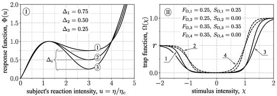
Figure 1. The characteristic functions describing (I) the subject’s actions in the critical situation and (II) the uncertainty in estimating the system state. The shown parameters are related to ansatz (9) for the function $\Phi \left(\eta \right)$ and ansatz (11) for the function $\Omega \left(\chi \right)$.

2.2.4. Concept of Dynamical Traps and the Governing Equation of Subject’s Actions

Because of uncertainty in the sensory perception, the subject may halt his active control over the system motion when the system comes close to the equilibrium $x=0$. Indeed, in this case, they just cannot recognize what specific actions are required and may prefer to change nothing in the state of their actions until the further system motion clarifies the needed changes. This type of behavior is often called human intermittent control, which manifests itself in that such control processes can be conceived of as a sequence of alternate fragments of passive and active phases in human actions. Nowadays, the intermittency of human control over external systems as well as inner processes responsible for the body equilibrium is considered an intrinsic property of human physiology [34]. The same concerns the mental estimation of the observed system dynamics. The subject may consider any change in their actions unnecessary if the difference between the current state and its alternative is ignorable in spite of being quite visible. In the case when the sensory perception is well balanced with the mental estimation, their similarity in uncertainty properties becomes pronounced, and we may suppose that the subject’s control based on mental evaluation is also characterized by the intermittency.

To allow for the accepted intermittency of the subject’s behavior, we turn to the concept of dynamical traps developed by Lubashevsky (see [35] for a detailed description). In particular, it generalizes the notion of the stationary point in describing dynamical systems governed by human actions. Namely, a stationary point is replaced by its certain neighborhood, where the corresponding “forces” caused by human actions become equal to zero. As a result, the dynamics of a system in issue is stagnated inside the dynamical trap region, and only random forces affect the system motion. A dynamical trap does not necessarily replace the corresponding stationary point; for a system with a multidimensional phase space, the dynamical trap can be related only to one of its dimensions and does not affect the system motion in the others.

In the present paper, we introduce a common model $\Omega \left(\chi \right)$ of dynamical traps affecting two state variables. One of them is the rate $\dot{x}$ normalized to the uncertainty ${\sigma }_{\dot{x}}$ of its mental estimation (Exp. (3)), namely, $\chi =\dot{x}/{\sigma }_{\dot{x}}$, representing the subject’s reaction to the stimulus related to $\dot{x}$. In this case, the dynamical trap effect is introduced via the following modification of Equation (5):

$$\frac{1}{\eta }\frac{d\eta }{dt}=\mu \Omega \left(\frac{\dot{x}}{\kappa \overline{v}}\right)\frac{\dot{x}}{\overline{x}}.$$

(10)

where, besides, the term $1/x$ is replaced by $1/\overline{x}$ containing no singularity at $x\to 0$. Inside the dynamical trap region $\left|\chi \right|\lesssim 1$, the stimulus, whose intensity is quantified by the variable $\chi$, is either not recognized by the subject or just ignored within its mental estimation. To specify the trap function $\Omega \left(\chi \right)$, we use the ansatz

$$\Omega \left(\chi \right)=\frac{1}{2}\left[rtanh\left(-\frac{\chi +1+S_{\Omega }}{F_{\Omega }}\right)+tanh\left(\frac{\chi -1-S_{\Omega }}{F_{\Omega }}\right)+(1+r)\right],$$

(11)

where the parameters $F_{\Omega }$ and $S_{\Omega }$ describe the fuzziness of the thresholds $\chi =\pm 1$ and their shift along the $\chi$-axis, respectively, the parameter $0<r\le 1$ allows for the subject to respond slower in decreasing its reaction intensity, i.e., when relaxing, in comparison with increasing intensity required to depress the system instability growth. Taking into account Figure 1II, we use the values $F_{\Omega }=S_{\Omega }=0.25$ in the numerical simulation; in this case, the size of the dynamical trap region (the region of “force depression,” $\Omega \left(\chi \right)\ll 1$) becomes actually equal to unity.

The other state variable

$$\chi ={\left[{\left(\frac{x}{x_c}\right)}^2+{\left(\frac{\eta }{{\eta }_c}\right)}^2\right]}^{1/2}$$

characterizes the subject’s estimation of the current state proximity to the critical situation when the probability of control failure is high and the subject reaction should be intensified urgently, which matches the values $\chi \gtrsim 1$. In this case, the dynamical trap effect is introduced via the following modification of Equation (8):

$$\frac{1}{\eta }\frac{d\eta }{dt}={\eta }_c\Omega \left\{\frac{1}{{\kappa }_c}{\left[{\left(\frac{x}{x_c}\right)}^2+{\left(\frac{\eta }{{\eta }_c}\right)}^2\right]}^{1/2}\right\}\left[\frac{x}{x_c}-\Phi \left(\frac{\eta }{{\eta }_c}\right)\right],$$

(12)

where the coefficient ${\kappa }_c\sim 1$ is a model parameter determined by the particular form of the trap function $\Omega \left(\chi \right)$.

Figure 2 visualizes the spatial structure of the right-hand-side functions of Equations (10) (panel I) and (12) (panel II). These functions are depicted via contour plots for $\kappa =0.25$ and ${\kappa }_c=1$. The domains on the corresponding planes that are free from level lines (except for the zero-level) illustrate the dynamical trap regions.

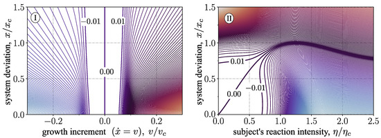
Figure 2. Illustration of the dynamical trap effects visualized via the contour plots of the right-hand-side functions of Equations (10) (I) and (12) (II). In plotting the parameters, $\kappa =0.25$ and ${\kappa }_c=1$ were used. The distance between the level lines is 0.01, blue and red tones represent negative and positive values of the visualized functions.

It should be noted that the concept of the dynamical trap was validated via comparison of the data collected in experiments on (i) balancing overdamped pendulums [36] and (ii) car-following dynamics based on a driving simulator, e.g., [37] (Section 7.6), with the corresponding results of numerical simulation.

2.2.5. Summary: The Governing Equation of Subject’s Actions ($\eta$-Dynamics)

Uniting Equation (10) with Equation (12) and taking into account random factors that are out of the subject’s control, we write the following equation describing the subject’s actions within the first-person perspective:

$$\begin{array}{c}\frac{1}{\eta }\frac{d\eta }{dt}=-{\rho }_r+{ϵ}_r\xi \left(t\right)+\mu \Omega \left\{\frac{\dot{x}}{\kappa \overline{v}}\right\}\frac{\dot{x}}{\overline{x}}\hfill \\ \hfill +{\eta }_c\Omega \left\{\frac{1}{{\kappa }_c}{\left[{\left(\frac{x}{x_c}\right)}^2+{\left(\frac{\eta }{{\eta }_c}\right)}^2\right]}^{1/2}\right\}\left[\frac{x}{x_c}-\Phi \left(\frac{\eta }{{\eta }_c}\right)\right],\end{array}$$

(13)

where the introduced first two terms on the right-hand side allow for (i) a slow decrease in the reaction intensity related to effort minimization when the necessity of active behavior is not clear, and (ii) uncontrollable fluctuations in the subject’s reaction. The parameters $0<{\rho }_r\ll 1$ and ${ϵ}_r\ll 1$ are the quantitative measures of the two factors. The white noise $\xi \left(t\right)$ is specified by the conditions

$$⟨\xi \left(t\right)⟩=0,⟨\xi \left(t\right)\xi \left(t^{\prime }\right)⟩=\delta (t-t^{\prime }).$$

The governing Equation (13) is actually the stochastic differential equation of the Stratonovich type, e.g., [38], written here in the form of a Langevin equation to elucidate its derivation based on the preceding mathematical constructions.

We want to emphasize that the constructed governing Equation (13) is actually a rather “simple” mathematical description of the subject’s behavior that takes into account the main features of human cognition affecting this type of human control. Indeed, we have the following:

–

The left-hand term $\dot{\eta }/\eta$, the stimuli for the subject’s active behavior quantified by $\dot{x}/\overline{x}$, $x/x_c$, and $\eta /{\eta }_c$ actually meet Weber’s law reflecting the scale-free properties of human perception;

–

The last two terms on the right-hand side just represent the two channels of the visual modality, processing separately sustained and transient information;

–

The dynamical trap function $\Omega (\dots )$ describes the subject’s intermittent behavior, in particular, the control stagnation when the subject is not able to recognize how the current state should be changed;

–

The first term on the right-hand side is due to the effort minimization when the subject’s active behavior is not necessary;

–

The introduced noise, the second term, allows for uncontrollable factors that are outside of the subject’s cognition.

The delay in human response to current external stimuli is actually taken into account by treating the quantity $\eta$—the characteristics of the subject’s internal state—as an independent phase variable.

3. Results of Numerical Simulation and Discussion

The system of Equations (1) and (13) is analyzed numerically using the order 1.0 strong stochastic Runge–Kutta algorithm SRS2 for Stratonovich equations that is elaborated by Rößler [39] and implemented in the Python library sdeint 0.3.0. To accumulate enough statistics, the integration time is set equal to $T={10}^5$, and the discretization step size is $dt=0.001$. In analyzing the accumulated data, the algorithms histogram and welch (with window size $8192=2^{13}$) of NumPy (version 1.22) and SciPy (version 1.8) are used for constructing the distributions of the variables x and $\eta$ and the corresponding power spectral densities.

3.1. The Used Model Parameters

We analyze two particular cases that make the contribution of either the fine-control mode or the critical-control mode most pronounced. Their common features are as follows. The system deviation x from the unstable equilibrium $x=0$ is measured in units of the critical deviation $x_c$ when the subject’s control becomes close to failure, which is reflected in setting $x_c=1$. The corresponding value ${\eta }_c$ of the subject’s reaction intensity is also set equal to ${\eta }_c=1$, which actually implies that the unit of dimensionless time is re-normalized and now time is measured in units of the reaction time ${\tau }_c$ when $x\sim x_c$. Under such conditions, the subject’s reaction intensity ${\eta }_b<1$ (or even ${\eta }_b\ll 1$) at the instability onset becomes a model parameter, taking different values in the analyzed cases.

As far as the system dynamics governed by Equation (1) is concerned, the cut-off parameter of the very small value of x is set equal to ${\theta }_b=0.01$. In other words, the subject is assumed to be able to decrease the system deviation x maximally to $x_{\min }\lesssim 1$% of $x_c$. It, on the one hand, enables us to avoid artificial effects caused by $x\to 0$; on the other hand, the effect of such small values of x on the analyzed phenomenon cannot be remarkable.

As far as the subject’s reaction dynamics governed by Equation (13) is concerned, first, the following parameters $\kappa =0.25$, $\Delta =0.75$, $F_{\Omega }=S_{\Omega }=0.25$ are used; their choice is in Section 2.2. We set the parameter $r=0$ of the dynamical trap function $\Omega (\dots )$ to accentuate the difference in the subject’s behavior when the reaction should be intensified to depress the instability growth and when the subject may relax to minimize the effort of keeping the reaction intensity high. The increment ${\rho }_r=0.25$ of the intensity drop represents the intermediate rate of the effort minimization in comparison with the reaction intensification in the case of instability growth.

Domination of the fine-control mode is found for ${\eta }_b=0.1$, ${ϵ}_r=0.2$, and ${\kappa }_c=1$. These parameters correspond to (i) a relatively wide region of the subject’s reaction intensity between the instability onset and the control failure and (ii) the uncontrollable noise of lower intensity, making the residence time in the trap relatively longer.

Domination of the critical-control mode is found for ${\eta }_b=0.5$, ${ϵ}_r=0.4$, and ${\kappa }_c=2$. These parameters correspond to the nearness of the instability onset and control failure and the uncontrollable noise of higher intensity. These features make the subject’s step-wise reaction to the increase in the system deviation $x\sim x_c$ more pronounced, partly due to ${\kappa }_c=2$ shifting the onset of the subject step-wise reaction deeper into the trap domain.

Let us discuss the obtained results in the two cases separately.

3.2. The Case of Fine-Control Dominance

Figure 3 represents the found characteristics of the system dynamics in the given case. In particular, Figure 3I,II illustrates properties of the time patterns $x\left(t\right)$ and $\eta \left(t\right)$. As seen, the dynamics of the instability-induced system fluctuations and the subject’s reaction intensity looks like some collection of segments combing similar oscillations and whose amplitudes undergo irregular variations from small values near $x_c=1$ and ${\eta }_b=0.1$ up to values comparable with $x_c$ and ${\eta }_c=1$, respectively. Nevertheless, under the given conditions, the subject’s step-wise reaction to the system deviation x is not detected, meaning the subject is able to control the instability development via adapting the reaction to the currently observed system deviation x and its rate $\dot{x}$.

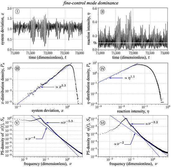
Figure 3. The characteristic properties of unstable system dynamics when the fine-control mode dominates. Panels I and II illustrate temporal patterns of the system deviation $x\left(t\right)$ from the unstable equilibrium $x=0$ (Panel I) and the subject’s reaction intensity $\eta \left(t\right)$ (Panel II). The horizontal white line ${\eta }_b=0.1$ (Panel II) visualizes the moments of instability onset. Panels III and IV exhibit the distribution functions $P_x$ and $P_{\eta }$ of the variables x (Panel III) and $\eta$ (Panel IV) constructed based on the generated data. The corresponding power-spectral densities (PS-densities or the distributions of spectral amplitudes) $S_x$ and $S_{\eta }$ are shown in Panels V and VI, respectively. To reveal the scale-free properties of the four distributions, log–log scales are used. Dashed blue lines visualize those fragments of these distributions that admit interpretation as a power-law dependence. The parameters used in numerical simulation are noted in Section 3.1.

Figure 3III,IV depict the distribution functions $P_x\left(x\right)$ and $P_{\eta }\left(\eta \right)$ of the variables x and $\eta$ in log–log scales that are constructed based on the generated time series $\left\{x\right(t\left)\right\}$ and $\left\{\eta \right(t\left)\right\}$. These distribution functions $P_x\left(x\right)$ and $P_{\eta }\left(\eta \right)$ actually represent the properties of irregular variations in the amplitudes of oscillation segments (Figure 3I,II) forming the time series $\left\{x\right(t\left)\right\}$ and $\left\{\eta \right(t\left)\right\}$. In the same way, Figure 3V,VI exhibit the corresponding power-spectral densities $S_x\left(\nu \right)$ and $S_{\eta }\left(\nu \right)$, characterizing the temporal properties of the time series $\left\{x\right(t\left)\right\}$ and $\left\{\eta \right(t\left)\right\}$. Let us remind that the power spectrum of a time series $\left\{\chi \right(t\left)\right\}$ describes the distribution of the squared amplitudes $|V_{\nu }{|}^2$ of the corresponding Fourier components $\left\{V_{\nu }\right\}$—harmonic oscillations $V_{\nu }exp\left(i2\pi \nu t\right)$ whose union makes up the time series $\left\{\eta \right(t\left)\right\}$. In this context, the variable $\nu$ may be treated as a dimensionless frequency.

To precisely reveal the possibility of identifying the scale-free fragments—admitting interpretation as a power-law dependence—of the four distributions $P_x$, $P_{\eta }$, $S_x$, and $S_{\eta }$, we turn to log-log plots. As seen in Figure 3III,IV, the growing fragments of the distribution function $P_x\left(x\right)$ and $P_{\eta }\left(\eta \right)$ do admit interpretation as power-law dependencies spanning over about two orders of magnitudes with respect to the values of these distributions and one order with respect to variations in their arguments. It should be emphasized that the scale-free fragment of the distribution function $P_{\eta }\left(\eta \right)$ belongs to the region $\eta <{\eta }_b=0.1$ of the instability onset. It can be explained as a result of the subject being in the relaxed state characterized by the minimal effort of just waiting until the system deviation x from the unstable equilibrium $x=0$ starts to grow remarkably. This conclusion is also justified by the power-law increase in the distribution function $P_x\left(x\right)$ that occurs in the region of $x<x_c$ below the critical value $x_c=1$.

Two power-law fragments can be also singled out in the power-spectral densities $S_x\left(\nu \right)$, $S_{\eta }\left(\nu \right)$ (Figure 3V,VI). We focus on the fragments adjacent to the density maxima; along the $\nu$-direction, these fragments span from ${\nu }_l\approx 0.05$ up to ${\nu }_u\approx 0.5$. The corresponding temporal scales can be estimated as $t\sim 1/\nu$, which leads to the dimensionless time interval $2\lesssim t\lesssim 20$ corresponding to time variations in the $x\eta$-cross correlations (in the present paper, we do not present the constructed function of the cross correlations). It is interesting that in the case of fine-control mode dominance, these fragments are followed by deeper fragments being also of the power-law type that is characterized by a weaker decrease. We relate this feature to the effect of white noise on the scale-free dynamics manifesting itself in the discussed above fragments.

3.3. The Case of Critical-Control Dominance

Figure 4 represents the found characteristics of the system dynamics in the given case. In particular, Figure 4I,II illustrate the properties of the time patterns $x\left(t\right)$ and $\eta \left(t\right)$. As seen, dynamics of the instability-induced system fluctuations looks like irregular step-wise variations in the system deviation x. These step-wise x-variations are due to spike-wise variations in the subject’s response to the system deviations $x\sim x_c$. For the given model parameters, such large-scale fluctuations in the variable x arise rather often and the subject has to depress them via the “urgent” step-wise reaction, whose description is based on Equation (13) with the N-type shape of the function $\Phi (\eta /{\eta }_c)$ (Figure 1I). The amplitudes of these spike-wise $\eta$-variations are also irregular.

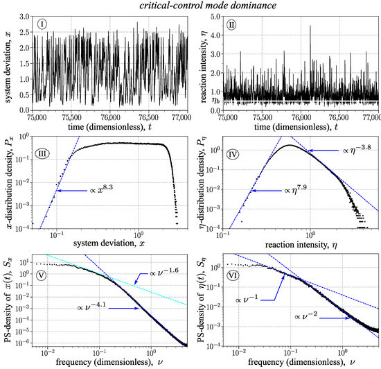
Figure 4. The characteristic properties of unstable system dynamics when the critical-control mode dominates. Panels I and II illustrate temporal patterns of the system deviation $x\left(t\right)$ from the unstable equilibrium $x=0$ (Panel I) and the subject’s reaction intensity $\eta \left(t\right)$ (Panel II). The horizontal white line ${\eta }_b=0.5$ (Panel II) visualizes the moments of instability onset. Panels III and IV exhibit the distribution functions $P_x$ and $P_{\eta }$ of the variables x (Panel III) and $\eta$ (Panel IV) constructed based on the generated data. The corresponding power-spectral densities (PS-densities or the distributions of spectral amplitudes) $S_x$ and $S_{\eta }$ are shown in Panels V and VI, respectively. To reveal the scale-free properties of the four distributions, log–log scales are used. Dashed blue lines visualize those fragments of these distributions that admit interpretation as a power-law dependence. The dashed cyan line in Panel V depicts the power-law dependence only approximating the corresponding fragment of the PS-density. The parameters used in numerical simulation are noted in Section 3.1.

The resulting distribution functions $P_x\left(x\right)$ and $P_{\eta }\left(\eta \right)$ are depicted in Figure 4II,IV again in log–log scales. As in the previous case (Section 3.2), both the distribution functions possess the increasing parts described by the power-law dependence, and these parts are located in the region where, on the one hand, the x-dynamics becomes unstable, $\eta <{\eta }_b=0.5$, and, on the other hand, the system deviation $x\ll x_c=1$ is not considerable yet. However, in contrast to the previous case, the subject’s step-wise response endows the distribution function $P_{\eta }\left(\eta \right)$ with an additional decreasing fragment of the power-law type (Figure 4IV). Its location along the $\eta$-axis is actually determined by the N-type shape of the function $\Phi (\eta /{\eta }_c)$ (Figure 1I).

As far as the power-spectral densities $S_x\left(\nu \right)$ and $S_{\eta }\left(\nu \right)$ (Figure 4V,VI) are concerned, their form is rather similar to the power-spectral densities obtained in the previous case. In particular, both of these PS-densities individually possess two fragments of the power-law type. As before, the time scales corresponding to the frequency domain of the power-law fragments adjacent to the PS-distribution maxima represent the time scales of the $x\eta$-cross-correlations.

The found difference is reduced to the fact that, first, the power-law form of the fragment adjacent to the maximum of the PS-density $S_x\left(\nu \right)$ is not pronounced. We explain this feature by the essential overlapping between two domains in the x-space characterized by different modes of system control. One of them is the domain $x\lesssim x_c=1$, where the fine-control mode should dominate over the critical-control mode. The other is the domain $x\gtrsim x_c$, where, in turn, the critical-control mode has to become dominant. As a result, the x-domain of this fragment shrinks to the region $0.02\lesssim x\lesssim 0.2$ and seems to lose the strict power-law form (Figure 4V).

Second, in the given case, the power-law fragments of the PS-densities following the discussed ones decrease with the dimensionless frequency $\nu$ faster. It corresponds to a more conventional form of PS-densities, where their deep tails are due to some mechanisms that inhibit the emergence of power-law dependencies. We consider the subject’s step-wise reaction caused by the system’s critical deviation to serve as such a breakdown mechanism.

4. Conclusions

The developed model for human control over an unstable system comprises two constituent components. One of them is the linear model for supercritical instability, where the control parameter, by which the subject is able to stabilize the system dynamics, is the intensity of the reaction. The other is the model for the subject’s behavior constructed based on the first-person perspective. It takes into account the basic properties of human cognition, determining the analyzed type of human control. Namely, they are as follows:

–

The scale-free properties of human perception of external stimuli underpinning, in particular, Weber’s law;

–

The multi-channel structure of sensory modalities processing the sustained and transient components of sensory information separately;

–

The bounded capacity of human cognition that gives rise to intermittent control and is responsible for the emergence of a certain region in the extended phase space, where the subject’s active behavior is stagnated;

–

The minimization of effort when the subject’s active behavior is not necessary;

–

The delay in human reaction taken into account via the introduction of the extended phase space consisting of (i) phase variables describing the states of a physical system under human control and (ii) phase variables describing the internal states of the subject.

The latter component of the proposed model is essentially its novel feature. Although Equation (13) governing the subject’s behavior seems to be complicated, its terms describe the given properties of human cognition in a rather simple way, catching only their basic aspects.

We would like to note that the experimental validation of the proposed approach is a matter of further research. However, its basic premises are grounded on available experimental data and verified theoretical constructions.

The proposed model is studied numerically. The constructed distributions of the phase variables and the corresponding power-spectral densities possess a variety of fragments admitting interpretation as the power-law dependences. It enables us to categorize the system dynamics governed by the given model as the self-organized criticality.1

As should be emphasized, the developed model deals with a single person and their adaptive control over an unstable system and predicts its complex dynamics exhibiting scale-free properties. It enables us to posit that the dynamic complexity of social systems is not only due to their multi-element structure. Social systems can also inherit some of their complex properties from the individual behavior of their members.

As a plausible application of the constructed approach, we may note the verification of a hypothesis about the emergence of the synchronized mode in highway traffic flow—the mode determining the number of fundamental properties of traffic flow and remaining challenging problems in traffic flow physics. The hypothesis states that the synchronized mode emerges via the described SOC scenario rather than the classic scenario of self-organization: the onset of instability, its development, and the resulting spatiotemporal patterns stabilized by nonlinear effects in system dynamics.

References

- Bak, P.; Tang, C.; Wiesenfeld, K. Self-Organized Criticality: An Explanation of 1/f Noise. Phys. Rev. Lett. 1987, 59, 381–384. [Google Scholar] [CrossRef] [PubMed]
- Marković, D.; Gros, C. Power laws and self-organized criticality in theory and nature. Phys. Rep. 2014, 536, 41–74. [Google Scholar] [CrossRef]
- Watkins, N.W.; Pruessner, G.; Chapman, S.C.; Crosby, N.B.; Jensen, H.J. 25 Years of Self-organized Criticality: Concepts and Controversies. Space Sci. Rev. 2016, 198, 3–44. [Google Scholar] [CrossRef]
- Muñoz, M.A. Colloquium: Criticality and dynamical scaling in living systems. Rev. Mod. Phys. 2018, 90, 031001. [Google Scholar] [CrossRef]
- Tadić, B.; Melnik, R. Self-Organised Critical Dynamics as a Key to Fundamental Features of Complexity in Physical, Biological, and Social Networks. Dynamics 2021, 1, 181–197. [Google Scholar] [CrossRef]
- Bonachela, J.A.; Muñoz, M.A. Self-organization without conservation: True or just apparent scale-invariance? J. Stat. Mech. Theory Exp. 2009, 2009, P09009. [Google Scholar] [CrossRef]
- Sornette, D. Sweeping of an instability: An alternative to self-organized criticality to get powerlaws without parameter tuning. J. Phys. I 1994, 4, 209–221. [Google Scholar] [CrossRef]
- Sornette, D. Critical Phenomena in Natural Sciences: Chaos, Fractals, Selforganization and Disorder: Concepts and Tools; Springer: Berlin/Heidelberg, Germany, 2006. [Google Scholar] [CrossRef]
- Kinouchi, O.; Brochini, L.; Costa, A.A.; Campos, J.G.F.; Copelli, M. Stochastic oscillations and dragon king avalanches in self-organized quasi-critical systems. Sci. Rep. 2019, 9, 3874. [Google Scholar] [CrossRef]
- Ramos, R.T.; Sassi, R.B.; Piqueira, J.R.C. Self-organized criticality and the predictability of human behavior. New Ideas Psychol. 2011, 29, 38–48. [Google Scholar] [CrossRef]
- Karsai, M.; Jo, H.H.; Kaski, K. Bursty Human Dynamics; Springer International Publishing AG: Cham, Switzerland, 2018. [Google Scholar] [CrossRef]
- Cabrera, J.L.; Milton, J.G. On-Off Intermittency in a Human Balancing Task. Phys. Rev. Lett. 2002, 89, 158702. [Google Scholar] [CrossRef]
- Cabrera, J.L.; Bormann, R.; Eurich, C.; Ohira, T.; Milton, J. State-Dependent Noise and Human Balance Control. Fluct. Noise Lett. 2004, 4, L107–L117. [Google Scholar] [CrossRef]
- Cabrera, J.L.; Milton, J.G. Human stick balancing: Tuning Lèvy flights to improve balance control. Chaos Interdiscip. J. Nonlinear Sci. 2004, 14, 691–698. [Google Scholar] [CrossRef] [PubMed]
- Nagatani, T. Power-Law Distribution and 1/f-Noise of Waiting Time near Traffic-Jam Threshold. J. Phys. Soc. Jpn. 1993, 62, 2533–2536. [Google Scholar] [CrossRef]
- Laval, J.A. Self-organized criticality of traffic flow: Implications for congestion management technologies. Transp. Res. Part C Emerg. Technol. 2023, 149, 104056. [Google Scholar] [CrossRef]
- Kerner, B.S. Introduction to Modern Traffic Flow Theory and Control: The Long Road to Three-Phase Traffic Theory; Springer: Berlin/Heidelberg, Germany, 2009. [Google Scholar] [CrossRef]
- Lubashevsky, I.; Morimura, K. Physics of Mind and Car-Following Problem. In Complex Dynamics of Traffic Management, Encyclopedia of Complexity and Systems Science Series; Kerner, B.S., Ed.; Springer Science+Business Media, LLC: New York, NY, USA, 2019; pp. 559–592. [Google Scholar] [CrossRef]
- Insperger, T.; Milton, J. Delay and Uncertainty in Human Balancing Tasks; Springer Nature Switzerland AG: Cham, Switzerland, 2021. [Google Scholar] [CrossRef]
- Suzuki, Y.; Morimoto, H.; Kiyono, K.; Morasso, P.G.; Nomura, T. Dynamic Determinants of the Uncontrolled Manifold during Human Quiet Stance. Front. Hum. Neurosci. 2016, 10, 618. [Google Scholar] [CrossRef]
- Lubashevsky, I.; Plavinska, N. Physics of the Human Temporality: Complex Present; Understanding Complex Systems; Springer International Publishing AG: Cham, Switzerland, 2021. [Google Scholar] [CrossRef]
- Helbing, D. Traffic and related self-driven many-particle systems. Rev. Mod. Phys. 2001, 73, 1067–1141. [Google Scholar] [CrossRef]
- Landau, L.D.; Lifshitz, E.M. Mechanics, 3rd ed.; Course of Theoretical Physics; Elsevier Butterworth-Heinemann: Burlington, MA, USA, 1976; Volume 1. [Google Scholar] [CrossRef]
- Patzelt, F.; Pawelzik, K. Criticality of Adaptive Control Dynamics. Phys. Rev. Lett. 2011, 107, 238103. [Google Scholar] [CrossRef]
- Gescheider, G.A. Psychophysics: The Fundamentals, 3rd ed.; Lawrence Erlbaum Associates: Mahwah, NJ, USA, 1997. [Google Scholar]
- Milton, J.; Meyer, R.; Zhvanetsky, M.; Ridge, S.; Insperger, T. Control at stability’s edge minimizes energetic costs: Expert stick balancing. J. R. Soc. Interface 2016, 13, 20160212. [Google Scholar] [CrossRef]
- Fu, C.; Suzuki, Y.; Morasso, P.; Nomura, T. Phase resetting and intermittent control at the edge of stability in a simple biped model generates 1/f-like gait cycle variability. Biol. Cybern. 2020, 114, 95–111. [Google Scholar] [CrossRef]
- Lubashevsky, I. Psychophysical laws as reflection of mental space properties. Phys. Life Rev. 2019, 31, 276–303. [Google Scholar] [CrossRef]
- Cowan, N. Sensational Memorability: Working Memory for Things We See, Hear, Feel, or Somehow Sense. In Mechanisms of Sensory Working Memory: Attention and Performance XXV; Jolicoeur, P., Lefebvre, C., Martinez-Trujillo, J., Eds.; Academic Press: San Diego, CA, USA, 2015; pp. 5–22. [Google Scholar] [CrossRef]
- Teghtsoonian, R. Range Effects in Psychophysical Scaling and a Revision of Stevens’ Law. Am. J. Psychol. 1973, 86, 3–27. [Google Scholar] [CrossRef] [PubMed]
- Stigliani, A.; Jeska, B.; Grill-Spector, K. Differential sustained and transient temporal processing across visual streams. PLoS Comput. Biol. 2019, 15, e1007011. [Google Scholar] [CrossRef]
- Wickelgren, W.A. Speed-accuracy tradeoff and information processing dynamics. Acta Psychol. 1977, 41, 67–85. [Google Scholar] [CrossRef]
- Cross, D.V. Sequential dependencies and regression in psychophysical judgments. Percept. Psychophys. 1973, 14, 547–552. [Google Scholar] [CrossRef]
- Loram, I.D.; Gollee, H.; Lakie, M.; Gawthrop, P.J. Human control of an inverted pendulum: Is continuous control necessary? Is intermittent control effective? Is intermittent control physiological? J. Physiol. 2011, 589, 307–324. [Google Scholar] [CrossRef]
- Lubashevsky, I. Human Fuzzy Rationality as a Novel Mechanism of Emergent Phenomena. In Handbook of Applications of Chaos Theory; Skiadas, C.H., Skiadas, C., Eds.; CRC Press: Boca Raton, FL, USA; Taylor & Francis Group: London, UK, 2016; pp. 827–878. [Google Scholar] [CrossRef]
- Zgonnikov, A.; Lubashevsky, I.; Kanemoto, S.; Miyazawa, T.; Suzuki, T. To react or not to react? Intrinsic stochasticity of human control in virtual stick balancing. J. R. Soc. Interface 2014, 11, 20140636. [Google Scholar] [CrossRef]
- Lubashevsky, I. Physics of the Human Mind; Springer International Publishing AG: Cham, Switzerland, 2017. [Google Scholar] [CrossRef]
- Gardiner, C.W. Handbook of Stochastic Methods: For Physics, Chemistry and the Natural Sciences, 3rd ed.; Springer: Berlin/Heidelberg, Germany, 2009. [Google Scholar]
- Rößler, A. Runge-Kutta Methods for the Strong Approximation of Solutions of Stochastic Differential Equations. SIAM J. Numer. Anal. 2010, 48, 922–952. [Google Scholar] [CrossRef]
- McAteer, R.T.J.; Aschwanden, M.J.; Dimitropoulou, M.; Georgoulis, M.K.; Pruessner, G.; Morales, L.; Ireland, J.; Abramenko, V. 25 Years of Self-organized Criticality: Numerical Detection Methods. Space Sci. Rev. 2015, 198, 217–266. [Google Scholar] [CrossRef]
Disclaimer/Publisher’s Note: The statements, opinions and data contained in all publications are solely those of the individual author(s) and contributor(s) and not of MDPI and/or the editor(s). MDPI and/or the editor(s) disclaim responsibility for any injury to people or property resulting from any ideas, methods, instructions or products referred to in the content. |
© 2023 by the authors. Licensee MDPI, Basel, Switzerland. This article is an open access article distributed under the terms and conditions of the Creative Commons Attribution (CC BY) license (https://creativecommons.org/licenses/by/4.0/).