Cutting Energy Consumption Modeling by Considering Tool Wear and Workpiece Material Properties for Multi-Objective Optimization of Machine Tools

Abstract

The increasing demand for energy is leading to global depletion of fossil fuels and growing environmental pressures, which are issues that need to be addressed. Machine tools are basic energy-consuming equipment in manufacturing systems. However, existing theoretical models ignore tool wear as well as workpiece material properties. This makes it difficult to further improve the accuracy of the model. Therefore, this study begins with the point of view of energy dissipation in the metal material removal process. A milling power model for computer numerical control (CNC) machines, considering tool wear and workpiece material properties during machining, is established. At the same time, milling is taken as the research object. A multi-objective cutting parameter optimization model is established to ensure the surface quality of the workpiece. In addition, the cutting energy consumption is taken into account in the developed models. Based on the multi-objective manta ray foraging optimization algorithm (MOMRFO), the Pareto-optimal solution set under multiple cutting conditions is solved. Finally, the experimental results of optimized parameters are compared with empirical parameters. The average prediction accuracy of the proposed energy consumption prediction model is above 91%. The experiments show that machining quality improves by optimizing the cutting parameters, with SEC, MRR, and Ra increasing by more than 44%, 53%, and 38%, respectively. The goals of reducing energy consumption and increasing productivity are achieved.

1. Introduction

In 2021, the IEA published its landmark report, Net Zero by 2050: A Roadmap for the Global Energy Sector. Since then, the energy sector has seen a major shift [1]. Economic development and environmental complexities are concomitant. As per ISO-14000 standards, industries should manage their adverse activities to limit environmental damage [2]. The manufacturing industry, as an important part of the industry, consumes a large amount of energy in the process of product manufacturing, causing serious environmental problems [3]. With the increasingly serious environmental problems, the green transformation of the manufacturing industry is considered a necessary path for future development. Machine tool is the most basic energy-consuming equipment in the manufacturing industry [4], which is accompanied by a large amount of energy consumption while carrying a heavy processing workload. Exploring the law of energy consumption of machine tools and establishing a more accurate energy consumption model to achieve the purpose of green manufacturing with energy saving and emission reduction has attracted extensive attention from industry and academia [5].

To achieve the green transition in manufacturing, many studies have made valuable contributions to reliable and accurate energy consumption prediction in recent years. From the perspective of thermodynamics, Gutowski et al. [6,7] simplified the input and output balance problems of the energy flows and material flows in the manufacturing process with concepts of entropy, enthalpy, and exergy. Their research put forward for the first time that there is a functional relationship between energy consumption and material removal rate (MRR) in machining. Kara et al. [8] proposed an empirical model, in which power is inversely proportional to MRR, and the model achieved high accuracy in predicting energy consumption on lathes and milling machines. Li et al. [9] further proposed a specific energy consumption (SEC) model, considering spindle speed in the air cutting condition.

Although the above empirical models perform well in terms of prediction accuracy, the machine tool energy consumption in the cutting process is considered to be a complex and dynamically changing process. These empirical models ignore the dynamic factors in complex machining conditions. The analysis of machine tool energy consumption is essential to understand the complex and dynamic energy consumption behavior of machine tools [10]. Newman et al. [11] showed that the same MRR can be obtained using different combinations of cutting parameters, but the actual measured energy consumption values are not the same.

Depending on the focus of variable selection in energy modeling, a large number of scholars have modeled energy consumption based on cutting forces, tool wear, metal deformation, and cutting parameters in the cutting process. Rodrigues and Coelho [12] proposed an SEC model for high-speed cutting and pointed out that tool geometry parameters can directly affect the cutting force and SEC. Pawar et al. [13] proposed an energy-saving optimization strategy based on milling force, which is used for milling variable surface geometry to reduce energy consumption in machining. Shao et al. [14] presented a face-milling energy consumption model. Li et al. [15] developed a milling power consumption model for CNC machine tools considering cutting conditions and tool wear. Liu et al. [16] found that tool wear has a significant effect on the net specific energy of cutting in precision milling. Taking into account tool wear, Li et al. [17] proposed an energy-efficient optimization of cutting parameters for batch machining of multi-featured parts. Bayoumi et al. [18] and Pramanik et al. [19] developed a theoretical energy consumption model based on plastic deformation of metals. Wang et al. [20] revealed the effects of tool and cutting depth on the chip deformation behavior and the associated energy consumption based on the finite element method (FEM). Tang et al. [21] took into account the energy consumption in the metal cutting process when analyzing the chip formation process and established the energy consumption field in the cutting deformation zone. Guo et al. [22] proposed a method to optimize the cutting parameters in finish turning by taking into account both energy consumption and surface roughness. In their study, it was pointed out that SEC is not only related to the cutting parameters but also to the size of the workpieces. Girish et al. [23] developed a multi-objective prediction model for minimizing energy consumption and surface roughness to obtain the optimum machining parameters. Chen et al. [24] proposed that energy consumption can be effectively reduced by correctly selecting the cutting parameters. The energy utilized at the cutting edge can be modeled as the specific cutting energy (SCE) [25].

Many different methods have been developed to search the Pareto front for multi-objective optimization (MOO) problems. Although different algorithms own different searching mechanisms, the common goal is to find out the Pareto front [26]. Mirjalili et al. [27] developed a multi-objective ant lion optimizer (MOALO). Experiments were conducted on engineering design problems. The results show that the algorithm is suitable for solving challenging real-world problems. Verma et al. [28] provided an extensive review of the MOO algorithm NSGA-II. Zhang et al. [29] proposed a multi-objective particle swarm optimizer based on a competition mechanism. Experiments showed that the optimizer has good performance in optimization quality and convergence speed. Combining the advantages of the genetic operators and iterative greedy heuristic algorithms, Lu et al. [30] designed a Pareto-based multi-objective hybrid iterative greedy algorithm. Moldovan et al. [31] proposed a multi-objective bifurcated grey wolf optimization method.

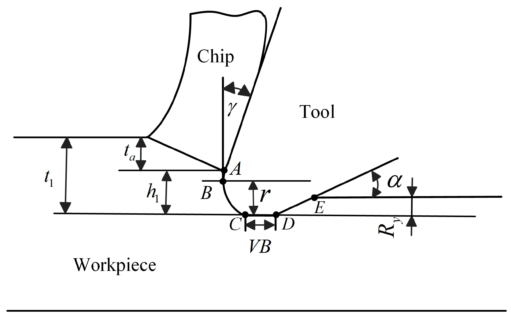
The above studies have focused on the physical factors arising from the tool and material in the machining process. Therefore, the influences of the unique internal material properties of cutting tools and workpieces on the energy changes in machining have been neglected. Inspired by this, a milling power consumption model that takes into account the workpiece material hardness and tool wear is developed in this study. On this basis, a multi-objective cutting parameter optimization model is established since the surface roughness of the machined material is often considered the main factor in measuring the machining quality. Afterward, based on the multi-objective optimization algorithm, the Pareto optimal solution set under multiple working conditions is solved.

The main original contributions of this study are as follows:

• The cutting power model of a three-axis CNC milling machine considering tool wear and workpiece material properties is established, and the prediction performance of the power model is verified. The influence mechanism of cutting parameters, tool wear, and workpiece material properties on cutting power are found.
• Taking milling processing as the research object, a multi-objective cutting parameter optimization model is established based on tool wear and workpiece material properties, with surface roughness, MRR, and SEC of the machining material as the optimization objectives.
• For the cutting parameter optimization model, the MOMRFO algorithm is introduced for the first time to solve the Pareto-optimal solution set under multiple working conditions. Under the premise of ensuring the machining quality, the optimal machining parameters that reduce energy consumption can be obtained.

The rest of this paper is organized as follows: Section 2 elaborates on the cutting power model considering workpiece hardness and tool wear. Experimental results and discussions are presented in Section 3. Section 4 presents the optimization model and algorithm of multi-objective cutting parameters. Finally, Section 5 concludes the paper and provides some future directions.

2. Modeling

From Figure 1, it can be seen that the metal cutting deformation zone can be divided into the first deformation zone, the second deformation zone, and the third deformation zone. The first deformation zone is the main deformation zone, and its main energy consumption is plastic deformation energy. The second deformation zone occurs in the chip and workpiece contact area, and its main energy consumption is the rake face friction energy. The third deformation zone occurs in the tool and workpiece contact area, and its main energy consumption is the flank face friction energy. Therefore, the energy consumption in the cutting process mainly consists of the following three parts: plastic deformation energy, rake face friction energy, and flank face friction energy. Energy consumption is an integral of power over time.

Figure 1. Metal cutting deformation zone.

2.1. Plastic Deformation Power Modeling Based on Workpiece Hardness

Plastic deformation energy is the strain energy consumed during plastic deformation in the first deformation zone, which can be expressed by the energy consumed per unit volume of material undergoing plastic deformation, as shown in Equation (1).

$$A_u={\displaystyle {\int }_o^{\epsilon }{\tau }_c\left(\epsilon ,\dot{\epsilon },T\right)\mathrm{d}\epsilon }$$

(1)

where $A_u$ is the plastic deformation energy, J/mm³. ${\tau }_c$ is the equivalent shear flow stress, MPa. $\epsilon$ is the shear strain. $\dot{\epsilon }$ is the shear strain rate, s⁻¹. $T$ is the temperature of the material.

The equivalent shear flow stress is calculated by the Johnson–Cook [32] constitutive model. It is suitable for the range of strain rates within 10² to 10⁶ s⁻¹. The equivalent flow stress in the Johnson–Cook constitutive model is calculated as shown in Equation (2).

$${\tau }_c=\frac{\sigma }{\sqrt{3}}=\frac{1}{\sqrt{3}}\left[A+B{\left(\frac{\epsilon }{\sqrt{3}}\right)}^n\right]\left[1+Cln\left(\frac{\dot{\epsilon }}{{\dot{\epsilon }}_0}\right)\right]\left[1-{\left(\frac{T-T_r}{T_m-T_r}\right)}^m\right]$$

(2)

where $\sigma$ is the equivalent flow stress. A, B, n, C, and m are the initial yield stress, hardening modulus, strain hardening coefficient, strain rate correlation coefficient, and thermal softening coefficient. They are generally obtained using Hopkinson compression rod experiments. ${\dot{\epsilon }}_0$ is the reference strain rate. T_m is the melting temperature of the workpiece material. T_r is the ambient temperature and T is the material temperature.

Equation (2) contains the elastic-plastic term $[A+B{(\epsilon /\sqrt{3})}^n]$, velocity term $[1+C\ln (\dot{\epsilon }/{\dot{\epsilon }}_0)]$, and thermal softening term $[1-{{(T-T_r)}^m/(T_m-T)}^m]$. The elasticity term is related to the mechanical properties of the material. Among the many properties of materials, hardness is a mechanical property index that integrates elasticity and strength. Material hardness can be approximated as a multiple of the ultimate tensile strength of the material, as shown in Equation (3).

$$H=k_h{\sigma }_s$$

(3)

where H is the Vickers hardness of the workpiece material, kgf/mm². ${\sigma }_s$ is the ultimate material tensile strength, MPa. k_h is the coefficient term, generally taken as 0.33.

As the chip flows through the first deformation zone, the chip undergoes severe plastic deformation and the temperature rises rapidly in the cutting zone. The material temperature T, which is located in the first deformation zone, can be calculated as the sum of the current ambient temperature T_r and the temperature increment $\Delta T$ due to plastic deformation, as shown in Equation (4).

$$T=T_r+\Delta T$$

(4)

The incremental temperature resulting from the effect of shear flow stress and shear strain is given in Equation (5).

$$\Delta T=T-T_r=\frac{\mu \eta {\displaystyle {\int }_o^{\epsilon }{\tau }_c\left(\epsilon ,\dot{\epsilon },T\right)\mathrm{d}\epsilon }}{{\rho }_m{c}_0}$$

(5)

where ${\rho }_m$ is the density of the material, g/cm³. $c_0$ is the specific heat capacity of the material, J/(g·°C). $\mu$ is the thermal distribution coefficient, cm³/s and $\eta$ is the coefficient of conversion of plastic work to an increase in temperature, also known as the Taylor coefficient or Quiney’s coefficient, which has a value of usually 0.9.

The heat distribution coefficient and heat diffusion coefficient are calculated as shown in Equations (6) and (7).

$$\mu =\frac{1}{1+1.328\sqrt{\frac{\lambda \epsilon }{v_c{t}_c}}}$$

(6)

$$\lambda =\frac{k_{\lambda }}{{\rho }_m{c}_0}$$

(7)

where $\lambda$ is the heat diffusion coefficient, m²/s. $t_c$ is the thickness of the undeformed chip, mm.

The temperature of the machined area within the shear zone can be considered an equivalent replacement for the tool temperature given by Kronenberg’s analysis [33]. The cutting tool temperature is given by Equation (8).

$$T=\frac{k_m{c}_v{\overline{\tau }}_c{v}_c^{o1}{a}_e^{o2}\cos \left(\beta -\gamma \right)}{\sin \varphi \sin \beta {\cos }^2\left(\varphi +\beta -\gamma \right)k_{\lambda }^{o3}{c}_0^{o4}}$$

(8)

where c_v is the Kronenberg constant [34]. ${\overline{\tau }}_c$ is the average shear stress in the main shear zone. $\beta$ is the friction angle. ${\gamma }_0$ is the cutting tool rake angle. $\varphi$ is the shear angle. k_m is the ratio of the actual contact length to the theoretical contact length.

The average stress ${\overline{\tau }}_c$ in the main shear zone is calculated as in Equation (9).

$${\overline{\tau }}_c=k_c{\sigma }_s$$

(9)

where k_c is generally 0.28.

Combining Equations (4)–(7), the plastic deformation energy can be obtained as Equation (10). The plastic deformation power model is shown in Equation (11).

$$\begin{array}{ll}{A}_u& ={\displaystyle {\int }_o^{\epsilon }\sigma \left(\epsilon ,\dot{\epsilon },T\right)\mathrm{d}\epsilon }=\frac{\left(T-T_r\right){\rho }_m{c}_0}{\eta \mu }\\ & =\frac{\left(\frac{k_m{k}_c{c}_{v}H{v}_c^{o1}{a}_e^{o2}\cos \left(\beta -\gamma \right)}{k_h\sin \varphi \sin \beta {\cos }^2\left(\varphi +\beta -\gamma \right)\cos k_{\lambda }^{o3}{c}_0^{o4}}-T_r\right)\left({\rho }_m{c}_0+1.328\sqrt{\frac{k_{\lambda }\epsilon }{v_c{a}_e}}\right)}{\eta }\end{array}$$

(10)

$$P_u=A_u{a}_p{a}_e{v}_f$$

(11)

2.2. Friction Power Modeling Based on Tool Wear

2.2.1. Friction Power on the Rake Face

When the cutting tool cuts the metal material in the second deformation zone, friction occurs when the chips flow out of the rake face, thus generating friction energy consumption. The friction between the chips and the rake face F is shown in Equation (12), and the friction energy of the rake face $A_{fl}$ is shown in Equation (13).

$$F=\frac{F_s\sin \beta }{\cos \left(\varphi +\beta -\gamma \right)}$$

(12)

$$A_{fl}=\frac{{\overline{\tau }}_{c}S{v}_{chip}\sin \beta }{v_c{t}_c{a}_e\cos \left(\varphi +\beta -\gamma \right)}$$

(13)

where $F_s$ is the shear deformation force. S is the contact area between the tool and the chip. v_chip is the chip flow speed. a_e is the cutting width. v_c is the cutting speed, which is expressed by $v_c=\pi dn/1000$. n is the spindle speed, and d is the cutting tool diameter.

The contact area of the cutting tool with the chip is $S=a_p{l}_c$, and the relationship between lc and the cutting width is given by Equation (14). The chip flow speed is calculated by Equation (15).

$$l_c=k_m\frac{a_p\sin \left(\varphi +\beta -\gamma \right)}{\sin \varphi \sin \beta }$$

(14)

$$v_{chip}=\frac{\sin \varphi }{\cos \left(\varphi -\gamma \right)}{v}_c$$

(15)

Combining (12)–(15), the calculation of the friction energy on the rake face can be obtained as Equation (16). The rake face friction power is modeled, as shown in Equation (17).

$$A_{fl}=\frac{H{k}_c{k}_m\sin \left(\varphi +\beta -\gamma \right)}{k_h\cos \left(\varphi +\beta -\gamma \right)\cos \left(\varphi -\gamma \right)}$$

(16)

$$P_{fl}=A_{fl}{a}_p{a}_e{v}_f$$

(17)

2.2.2. Friction Power of Flank Face

When the flank face of the cutting tool is worn, the friction between the flank face and the machined surface increases. Contact length between the flank face and the machined surface is expressed by l_ff, the average friction stress in the contact area is τ_cf, and the friction force acting in the contact area is $t_{cf}{l}_{ff}b$. Therefore, the friction energy on the flank face is shown in Equation (18).

$$A_{ff}=\frac{{\tau }_{cf}b{l}_{ff}{v}_c}{a_p{a}_e{v}_f}$$

(18)

Stress distribution law at the contact interface of the flank face can be expressed by ${\tau }_{cf}={\tau }_y\exp [-3{(x/\Delta )}^2]$, where ${\tau }_y$ is the shear strength of the material, and x is the distance from the cutting edge [34]. The average shear stress at the interface between the flank face and the workpiece contact area is obtained by integration ${\tau }_{cf}\left(x\right)=0.505{\tau }_y$.

When the cutting tools with a blunt is worn, the contact area between the cutting tool and the workpiece is shown in Figure 2. When the cutting tool cuts the workpiece, the contact length l_ff between the cutting tool and the workpiece is the circular arc AC, the horizontal line CD, and the inclined line DE, and the contact length between the cutting tool and the workpiece is calculated as in Equation (19).

$$l_{ff}=r\left(\arccos \left(1-\frac{h_1}{r}\right)-\arcsin \frac{VB-h_{re}\cot \gamma }{r}\right)+VB+\frac{h_{re}}{\sin \alpha }$$

(19)

where $\alpha$ is the back angle. VB is the wear width of the flank face. r is the radius of the cutting tool with blunt. h₁ is the height of the cutting tool with the blunt in contact with the workpiece arc. $\psi$ is the length of the cutting tool with a blunt in contact with the workpiece arc.

Figure 2. Contact area diagram of blunt tool and workpiece.

In the cutting process of the plastic deformation layer, there is $h_1/r\le 0.5-{\tau }_m/{\sigma }_{YT}$. Where ${\tau }_m$ and ${\sigma }_{YT}$ are the yield strength of the workpiece material and the strength of the bond between the cutting tool and the workpiece, respectively. The experiment results of cutting plastic materials show that the plastic deformation surface layer can be expressed by the polishing factor m = h₁/h_re;

Where h_re is the height of the residual area during the cutting process as shown in Figure 3.

Figure 3. Cutting residual height of three-edge end mill in the cutting process.

Rz is the maximum height of the contour in the roughness value. It is in the benchmark length of the contour curve, the highest point, and the lowest point of the sum of the distance. When cutting brittle materials or plastic materials at high speeds, the heights of the two are roughly equal. That is $h_{re}=Rz\approx 4Ra$. Combining Equation (19) yields the flank face friction-specific energy Equation (20).

$$A_{ff}=\frac{0.5{\tau }_y{v}_c\left(4Ra\cot \alpha +VB+r\left(\frac{\pi }{3}-\arcsin \frac{VB-4R_a\cot \gamma }{r}\right)\right)}{a_p{v}_f}$$

(20)

where R_a is the arithmetic mean deviation of the profile in the roughness value.

From Equation (20), when the cutting tool with rounded corners undergoes wear, the flank face friction power generated in the contact area between the cutting tool and the workpiece is shown in Equation (21). The tool-workpiece contact area after sharp-edged tool wear is shown in Figure 4.

$$P_{ff}=0.5{\tau }_y{a}_e{v}_c\left(4Ra\cot \alpha +VB+r\left(\frac{\pi }{3}-\arcsin \frac{VB-4R_a\cot \gamma }{r}\right)\right)$$

(21)

Figure 4. The tool-workpiece contact area after the sharp-edge tool wear.

The flank face friction power generated in the tool-workpiece contact area when wear occurs for a sharp-edged cutting tool is shown in Equation (22). The cutting power formula is as Equation (23).

$$P_{ff}={\tau }_y{a}_e{v}_c\left(4Ra\cot \alpha +VB\right)$$

(22)

$$P_c=P_u+P_{fl}+P_{ff}$$

(23)

The cutting tools used in this study are sharp-edged, so the friction power of the flank face is calculated using Equation (22). Combining Equations (11)–(23), the cutting power prediction model can be obtained as Equation (24).

$$\begin{array}{ll}{P}_c& =\frac{a_p{a}_e{v}_f}{\eta }\left(\frac{k_m{k}_c{c}_{v}H{v}_c^{o1}{a}_e^{o2}\cos \left(\beta -\gamma \right)}{k_h\sin \varphi \sin \beta {\cos }^2\left(\varphi +\beta -\gamma \right)\cos k_{\lambda }^{o3}{c}_0^{o4}}-T_0\right)\\ & \left({\rho }_m{c}_0+1.328\sqrt{\frac{{\rho }_m{c}_0\lambda \epsilon }{v_c{a}_e}}\right)+\frac{H{k}_c{k}_m\sin \left(\varphi +\beta -\gamma \right)a_p{a}_e{v}_f}{k_h\cos \left(\varphi +\beta -\gamma \right)\cos \left(\varphi -\gamma \right)}\\ & +{\tau }_y{a}_e{v}_c\left(4Ra\cot \alpha +VB\right)\end{array}$$

(24)

3. Experimental Verification

3.1. Design of the Experiment

The VDL-1000E machine tool (Dalian Machine Tool Group Corp., Dalian, China) was used for the cutting experiments in this study. The cutting power was collected by a power data acquisition device and compared with the predicted value of the cutting power model established in this study. The model validity was verified by calculating the prediction accuracy of the model. The cutting tool used for the experiments is shown in Figure 5. The specific parameters of the cutting tools are shown in Table 1. The machine tool, power monitoring, and data acquisition system are shown in Figure 6 and Figure 7 respectively.

Figure 5. Carbide end mill.

Table 1. Detailed information about the cutting tools.

Information	Parameter
Cutting tools	AL-3EL-D10
Material	tungsten steel
Tooth	3
Diameter	10 mm
Cutting edge length	45 mm
helix angle	45°

Figure 6. Three-axis CNC milling machine.

Figure 7. Power monitoring and data acquisition system.

Under the same cutting parameters, the measured and fitted values of cutting power are compared. The accuracy of the model prediction can be obtained. The effectiveness of the model is measured according to the prediction accuracy, as shown in Equation (25).

$$Acc=1-\frac{\left|P_m-P_p\right|}{P_m}$$

(25)

where P_p is the predicted value of cutting power. P_m is the measured value of cutting power. Acc is the fitting accuracy of the model.

In this study, the wiring diagram of the machine tool energy consumption measurement system is shown in Figure 8, the upper limit of the data acquisition frequency of the power monitoring and data acquisition system is 5 KHz. Its specific performance parameters are shown in Table 2. The specific parameters of the experimental instrument and material are shown in Table 3. The specific parameters of the workpieces are shown in Table 4 and Table 5.

Figure 8. Wiring diagram of machine tool energy consumption measurement system.

Table 2. Performance parameters of energy consumption measurement system.

Instrument Performance	Parameter
Acquisition system range	±10 V
Synchronous sampling rate	>50 kS/s
Acquisition accuracy	<1.5 m
Voltage transformer precision	0.2%
Current transformer precision	0.2%
Temperature range	−40 °C–+70 °C

Table 3. Detailed specification.

Parameters	Information
Machine tool	VDL-1000E
Ultra-depth field microscopy	PZ-ZC3500A
Workpiece material	6061-T6 2A12-T4 7075-T6
Size of workpiece	100 × 100 × 100 mm3 100 × 100 × 50 mm3 100 × 100 × 50 mm3
Cutting tool material	Carbide vertical milling cutter
Type	AL-3EL-D10.0
Cutting conditions	Dry

Table 4. Physical and mechanical properties of aluminum alloy.

Major Properties	6061-T6	2A12-T4	7075-T6
Tensile strength	310 MPa	230 MPa	524 MPa
Yield strength	240 MPa	42 MPa	455 MPa
Hardness HB	91.3 (kgf/mm2)	115.7 (kgf/mm2)	147.2 (kgf/mm2)
Elastic modulus	68.9 GPa	72.4 GPa	71.7 GPa

Table 5. Chemical properties of aluminum alloy.

Major Properties	6061-T6	2A12-T4	7075-T6
Al	Bal.	Bal.	Bal.
Cu	0.15%–0.4%	3.8%–4.9%	2.5%
Mn	0.15%	0.3%–0.9%	<0.1%
Mg	0.8%–0.12%	1.2%–1.8%	2.1%
Si	0.4%–0.8%	0.5%	<0.1%
Zn	<0.1%	0.3%	5.1%
Ti	<0.1%	0.15%	0.2%
Ni	<0.1%	<0.1%	<0.1%
Fe	<0.1%	<0.1%	0.3%

A total of 49 groups of 6 factors and 3 levels of milling experiments were designed by Minitab. The 6 factors were spindle speed n, feed rate v_f, cutting width a_e, cutting depth a_p, material hardness H, and tool wear VB, respectively. Specific parameters are shown in Table 6. The three levels of material hardness were achieved by selecting three aluminum alloys with different hardnesses: Al6061-T6, 2A12-T4, and 7075-T6.

Table 6. Cutting parameters of each level value.

Test	n (rpm)	vf (mm/min)	ap (mm)	ae (mm)	H (kgf/mm2)	VB (μm)
1	1200	100	1	2	91.3	38
2	1400	120	2	3	115.7	72
3	1600	140	3	4	147.2	113

Three levels of tool wear were achieved by selecting three cutting tools with different levels of flank face wear. The width of the flank face wear VB of the three cutting tools is shown in Figure 9, Figure 10 and Figure 11. For more details on tool wear, please refer to the work of Özbek [35]. The values of each level of the cutting parameters used specifically for the experiment are shown in Table A1. The cutting parameters were brought into the cutting power model to solve for the predicted values of cutting power, and the results of the measured cutting power are shown in Table A2.

Figure 9. The first level flank face wear width.

Figure 10. The second level flank face wear width.

Figure 11. The third level flank face wear width.

3.2. Experiment’s Validation

The experiment’s environmental temperature is T_r = 20 °C. The three types of workpiece material are aluminum alloys, with basically the same specific heat capacity, density, and thermal conductivity. The average value of density of the three is taken as ρ_m = 0.906 g/cm³, the specific heat capacity is C₀ = 2.759 J/(g·K), and the thermal conductivity is k_λ = 181 W/(m·K). The 49 groups of experiments data were obtained through milling experiments as shown in Table A1. The cutting power model was fitted by MATLAB according to the data in Table A2. Then cutting power model can be obtained in Equation (26).

The coefficient of determination of the cutting power model is R² = 0.9354. Based on the fitted cutting power model and the cutting parameters in Table A1, the model fitting results for the same cutting parameters are solved. The fitted accuracy of the solved model is shown in Table A2. The fitted results of cutting power are shown in Figure 12. The average fitted accuracy of cutting power is 92.40% and the minimum fitted accuracy is 87.47%. The data of the 47th, 48th, and 49th experiments were selected for validating the accuracy of the cutting power prediction model and the results are shown in Table 7.

$$\begin{array}{l}{P}_c=0.9a_e{a}_p{v}_f\left(3.471\times {10}^{-4}H{n}^{-2.129\times {10}^{-4}}{a_e}^{-0.542}-20\right)\\ \left(2.6936+\left(4.780\times {10}^{-2}/{\left(a_{\mathrm{e}}n\right)}^{0.5}\right)\right)+48.482a_e{a}_p{v}_f\\ +2.786\times {10}^{-5}{a}_{e}n\left(VB-3.958\times Ra\right)\end{array}$$

(26)

Figure 12. The predicted value of cutting power and the experimental value.

Table 7. Verification results of cutting power model.

Test	Pm (W)	Pp (W)	Acc (%)
1	47.825	43.711	91.40
2	77.955	70.325	90.21
3	54.445	50.955	93.59

3.3. Experiment Analysis

The prediction accuracy of the cutting power model established in this study is above 90%. The causes of errors are analyzed as follows: (1) The temperature in the shear deformation zone of the model is equivalent to the temperature of the cutting tool in the cutting process, but part of the heat generated in the cutting deformation zone will be taken away by the chips, thus generating errors. (2) The cutting energy consumption in the material removal process not only includes plastic deformation energy and friction energy, but also includes the generating new surface energy, elastic deformation energy, chip flow energy, and so forth. The reason for ignoring those is because it occupies too small a percentage of energy consumption, which is one of the reasons for the error.

The main effect of cutting power plotted from the experimental data is shown in Figure 13. The following conclusions can be drawn: a_p has the largest effect on cutting power, followed by a_e, then H, v_f, and VB, and the smallest effect is n.

Figure 13. Main effect diagram of cutting power. (a) Cutting parameters as horizontal coordinates. (b) Material hardness and flank face wear as horizontal coordinates.

Surface roughness reflects the height of the cutting residual surface on the workpiece surface. From Figure 14, it can be seen that SCE generally decreases with the increase in surface roughness. This means that the less energy consumed for removing a unit volume of material, the greater the surface roughness after machining.

Figure 14. The change trend of SCE with surface roughness.

4. Optimization

4.1. Multi-Objective Optimization Modeling

The surface roughness is considered an important indicator of machining quality. However, the machining process often requires multiple passes to obtain a relatively high surface quality, which also leads to higher machine tool energy consumption. To find the optimal machining parameters, this study establishes a three-objective optimization function with SEC, MRR, and Ra as the optimization objectives respectively. Under the premise of satisfying the machining quality of the workpiece, the energy consumption of the machining process is reduced to achieve energy saving (the details are shown in Table 8), where $P_{\mathrm{spi}}$ is the spindle power, which is divided into high-speed rotation power and low-speed rotation power. It is a linear function of spindle speed [9]. $P_{xf}$, $P_{yf}$ and $P_{zdf}$ are the X/Y/Z feed axis power respectively, which are quadratic functions of the feed speed v_f. $P_{zuf}$ is the spindle tool lifting power, which is a linear function of the feed speed v_f. $Ra$ is the surface roughness of the workpiece. This study is based on the response surface methodology (RSM) to establish its objective function. Each coefficient in the formula in Table 5 is a fitting coefficient. The specific parameters used for the equation fitting are shown in Table A3, Table A4, Table A5, Table A6, Table A7 and Table A8.

Table 8. Detailed specification.

Parameters	Mathematical Expression
Objective function (1)	$SEC=(595+P_{\mathrm{spi}}+P_{xf}+P_{yf}+P_{zuf}+P_{zdf}+P_c)/MRR$
	$P_{spi}=\left\{\begin{array}{c}\begin{array}{cc}0.1458\times n+5.603& n\in \left[100,1500\right]\end{array}\\ \begin{array}{cc}0.0755\times n+127.137& n\in \left(\left.1500,3000\right]\right.\end{array}\end{array}\right.$
	$P_{xf}=9.139\times {10}^{-6}\times {v_{xf}}^2+1.690\times {10}^{-2}\times v_{xf}+4.388$ $P_{yf}=7.583\times {10}^{-6}\times {v_{yf}}^2+1.534\times {10}^{-2}\times v_{yf}+6.744$ $P_{zdf}=-8.184\times {10}^{-7}\times {v_{zdf}}^2-8.824\times {10}^{-3}\times v_{zdf}+182.016$ $P_{zuf}=0.1031\times v_{zuf}+194.691$
Objective function (2)	$MRR=\frac{1000z{v}_c}{\pi d}{f}_z{a}_p{a}_e$
Objective function (3)	$\begin{array}{l}{R}_a=4.813+0.395a_p-2.741\times {10}^{-3}n+6.872\times {10}^{-4}{v}_f\\ -1.622\times {10}^{-2}{a}_p^2+4.733\times {10}^{-7}{n}^2-2.594\times {10}^{-7}{v}_f^2\\ -5.713\times {10}^{-5}{a}_{p}n+1.421\times {10}^{-5}{a}_p{v}_f-1.153\times {10}^{-7}n{v}_f\end{array}$

According to the three-objective optimization model established, combined with the actual experimental conditions, the mathematical model of the optimization constraints in this study was established as follows.

$$\left\{\begin{array}{l}{n}_{cutting}^{\min }\le n\le n_{cutting}^{\max }\\ f_z^{\min }\le f_z\le f_z^{\max }\\ a_p^{\min }\le a_p\le a_p^{\max }\\ a_e^{\min }\le a_e\le a_e^{\max }\\ Ra\le R{a}^{\max }\\ P_{cuttng}\le \eta P_m\end{array}\right.$$

(27)

Where n^min and n^max are the rated speed ranges of the spindle of the CNC machine used in this study. $f_z^{\min }$ and $f_z^{\max }$ are the ranges of the feed rate per tooth being restricted by the CNC machine. $a_p^{\min }$ and $a_p^{\max }$ are the ranges of cutting depth, $a_e^{min}$ and $a_e^{\max }$ are the ranges of cutting width, all of which need to be set by taking into account the performance of the machine tool, the materials and dimensions of the tool, and the workpiece. Ra^max is the maximum permissible surface roughness of the workpiece to be machined. η is the effective power factor and P_m is the rated power of the CNC machine tool.

4.2. MOMRFO Algorithm and Cutting Parameter Optimization Process

In this study, a MOMRFO [36] was used to optimize the developed multi-objective cutting parameter optimization model. MOMRFO is an improved multi-objective version based on MRFO [37].

The inspiration for this algorithm is based on the intelligent behaviors of manta rays. This work mimics three unique foraging strategies of manta rays, including chain foraging, cyclone foraging, and somersault foraging. For MOMRFO, the elitist concept is adopted to save the set of Pareto solutions through the integration of an external archive into the standard MRFO. It showed good promise in solving real-world problems with multiple objectives. MOMRFO mainly describes three behaviors as follows.

• Chain foraging.

This can be seen in Equation (28), where $x_i^t$ represents the t-th generation and the position of the i-th individual on the dimension and r represents a random number uniformly distributed in [0,1]. G_best represents the global best solution within the entire population. N is the size of the population.

$$x_i^{t+1}=\left\{\begin{array}{c}{x}_i^t+r.(G_{best}^t-x_i^t)+2.r.\sqrt{\left|\log (r)\right|}.(G_{best}^t-x_i^t)\begin{array}{cc}& \end{array}i=1\\ x_i^t+r.(x_{i-1}^t-x_i^t)+2.r.\sqrt{\left|\log (r)\right|}.(G_{best}^t-x_i^t)\begin{array}{cc}& \end{array}i=2,\dots ,N\end{array}\right.$$

(28)

2.

Helix foraging.

This can be seen from Equation (29), where T_max is the total number of iterations and t/T_max ≤ rand.

$$x_i^{t+1}=\left\{\begin{array}{c}{G}_{best}+r.(G_{best}^t-x_i^t)+2e^{r_1\frac{T_{\max }-t+1}{T_{\max }}}.\sin (2\pi r_1)(G_{best}^t-x_i^t),\begin{array}{cc}& \end{array}i=1\\ G_{best}+r.(x_{i-1}^t-x_i^t)+2e^{r_1\frac{T_{\max }-t+1}{T_{\max }}}.\sin (2\pi r_1)(G_{best}^t-x_i^t),\begin{array}{cc}& \end{array}i=2,\dots ,N\end{array}\right.$$

(29)

This can be seen from Equation (30), where x_rand is a random reference point in the search space given by Equation (31).

$$x_i^{t+1}=\left\{\begin{array}{c}{x}_{rand}+r.(x_{rand}^t-x_i^t)+2e^{r_1\frac{T_{\max }-t+1}{T_{\max }}}.\sin (2\pi r_1)(x_{rand}^t-x_i^t),\begin{array}{cc}& \end{array}i=1\\ x_{rand}+r.(x_{i-1}^t-x_i^t)+2e^{r_1\frac{T_{\max }-t+1}{T_{\max }}}.\sin (2\pi r_1)(G_{best}^t-x_i^t),\begin{array}{cc}& \end{array}i=2,\dots ,N\end{array}\right.$$

(30)

$$x_{rand}=LB+r.(UB-LB)$$

(31)

where LB and UB stand for the lower and upper boundaries of the search space, respectively.

3.

Tumbling foraging.

$$x_i^{t+1}=x_i^t+Q.(r_2.G_{best}-r_3.x_i^t),\begin{array}{cc}& \end{array}i=,\dots ,N$$

(32)

where Q is the somersault factor that defines the somersault range of manta rays. r₂ and r₃ are the same as r.

MOMRFO’s optimization process (Table 9) for the three-objective model developed for this study is shown below.

Table 9. MOMRFO’s optimization process.

Pseudo Code of the MOMRFO
CLC; CLEAR ALL
$\mathbf{Set}\mathbf{objective}\mathbf{function}\mathbf{:}\left\{\begin{array}{c}SEC\\ 1/MRR\\ P_c\end{array}\right.$
$\mathbf{Where}SEC=(595+P_{\mathrm{spi}}+P_{xf}+P_{yf}+P_{zuf}+P_{zdf}+P_c)/MRR$
/*Set the parameters of MOMRFO*/
Parameters:
Set Maxlt = 500 (the number of iterations is 100)
Set Pop_size = 100 (the population of manta rays is 100)
Set Ar_size = 100 (the maximum size of the archive)
Set beta = 4; Set nGird = 30; Set alpha = 0.1; Set gamma = 2
/*Executes the main structure of MOMRFO*/
WHILE (t < Maxlt) DO
If rand > 0.5
$\mathbf{If}\frac{t}{iter\_\max }$ < rand
Select xrand from POP using Equation (31)
Update the position using Equation (30)
else
DO Spiral foraging using Equation (29)
end
else
DO Chain foraging using Equation (28)
/*Update the Optimal Location*/
DO Tumbling foraging using Equation (32) and Update Location
END IF
To Cycle Again
END WHILE
RETURN the final archive Ar

4.3. Cutting Parameter Optimization Results and Verification

In this study, the problem of multidimensional selection of machining parameters due to multiple working conditions in real machining is considered. Three groups of 46 milling experiments with different machining parameters were selected as the comparison experiments before optimization. The MOMRFO algorithm was run by MATLAB. The comparison of cutting parameters before and after optimization as well as the objective function are listed in Table 10. The last row of Table 10 shows the recommended processing parameters optimized by MOMRFO, where n, v_f, a_e, and a_p are 3000, 600, 4, and 1, respectively, SEC and Ra reach their minimum values and MRR reaches its maximum value (the smaller SEC represents the less amount of energy consumed per unit volume of a workpiece cut during machining. Ra represents the surface quality of the material being machined; the smaller it is, the higher the surface quality. MRR represents the rate per unit volume removed; the larger it is, the faster the machining speed is). The last line is the optimized parameter. The optimized percentage improvement in SEC, MRR, and Ra compared to the pre-optimized set of three experiments is shown in Table 11. The optimally selected ranges are shown in Table 12.

Table 10. Comparison of values before and after optimization.

	n (r/min)	vf (mm/min)	ae (mm)	ap (mm)	SEC (J/mm3)	MRR (mm3/s)	Ra (μm)
1	1200	140	2	4	43.47	18.67	2.33
2	1600	100	2	4	71.44	13.33	1.73
3	1400	120	2	3	58.58	16	2.37
Opt.	3000	600	4	1	24.17	40	1.06

Table 11. SEC, MRR, R_a optimization improvement percentage.

	SEC (J/mm3)	MRR (mm3/s)	Ra (μm)
1	44.40%	53.32%	54.51%
2	66.17%	66.68%	38.73%
3	58.74%	60.00%	55.27%

Table 12. MOMRFO optimization parameter selection range.

	Parameter Range
ap	1–6 (mm)
ae	1–4 (mm)
vf	1–600 (mm/min)
n	1000–3000 (r/min)

5. Conclusions

In this study, a cutting power model for a three-axis CNC milling machine considering material properties and tool wear is proposed. The prediction accuracy of the cutting power model is verified through milling experiments. The proposed multi-objective function is optimized to obtain the optimal machining parameters. The following conclusions are drawn from this study.

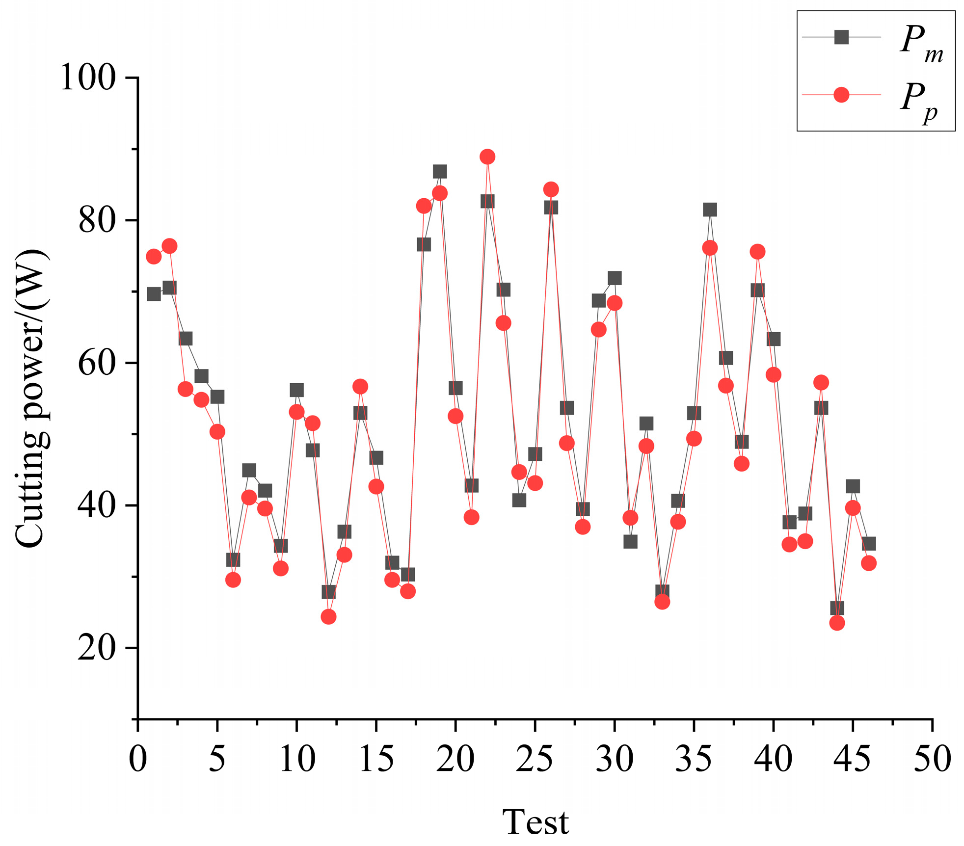
• A cutting power prediction model is established, which contains the material plastic deformation power, the rake face friction power, and the flank face friction power. As verified through experiments, the prediction accuracy of the developed model in this study is above 90%.
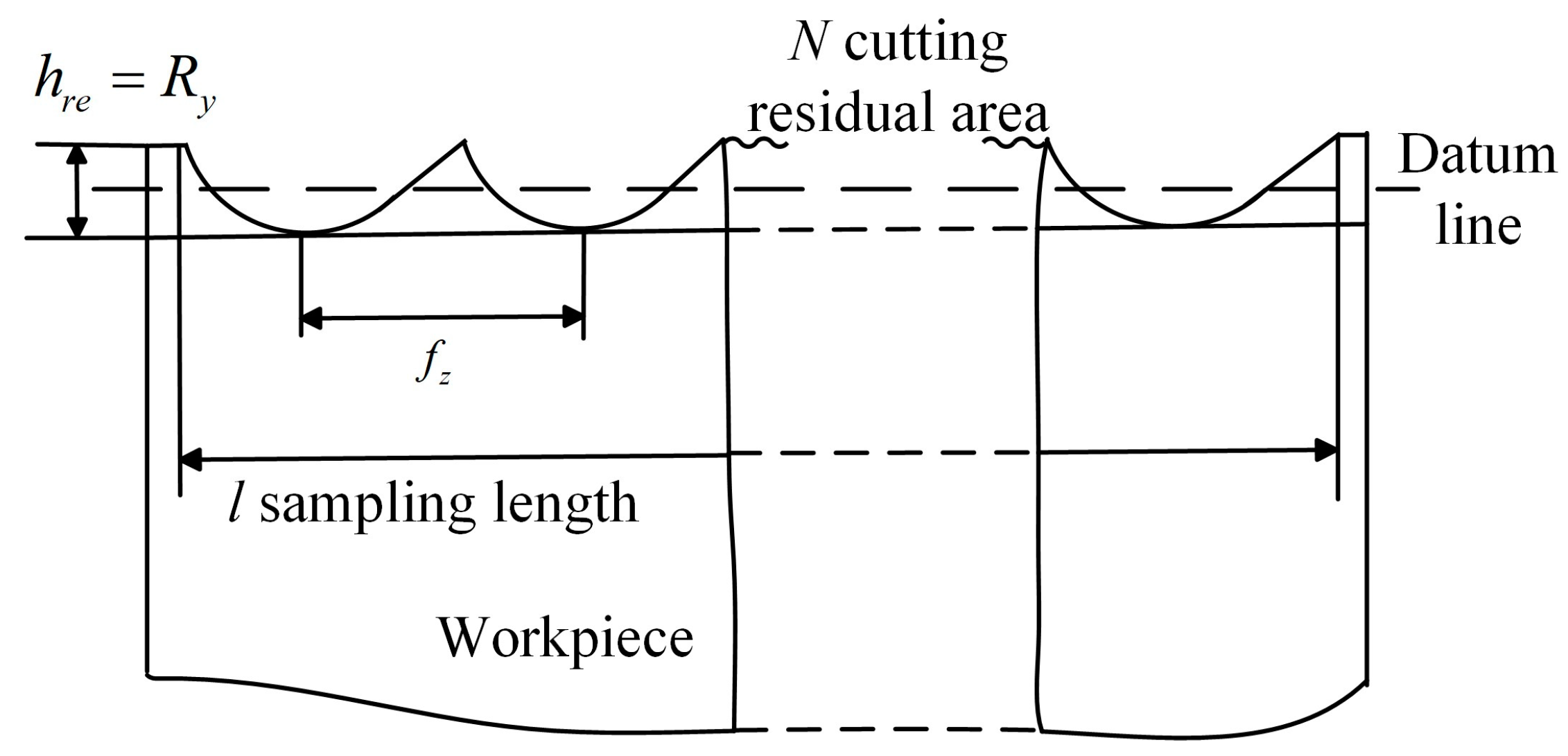
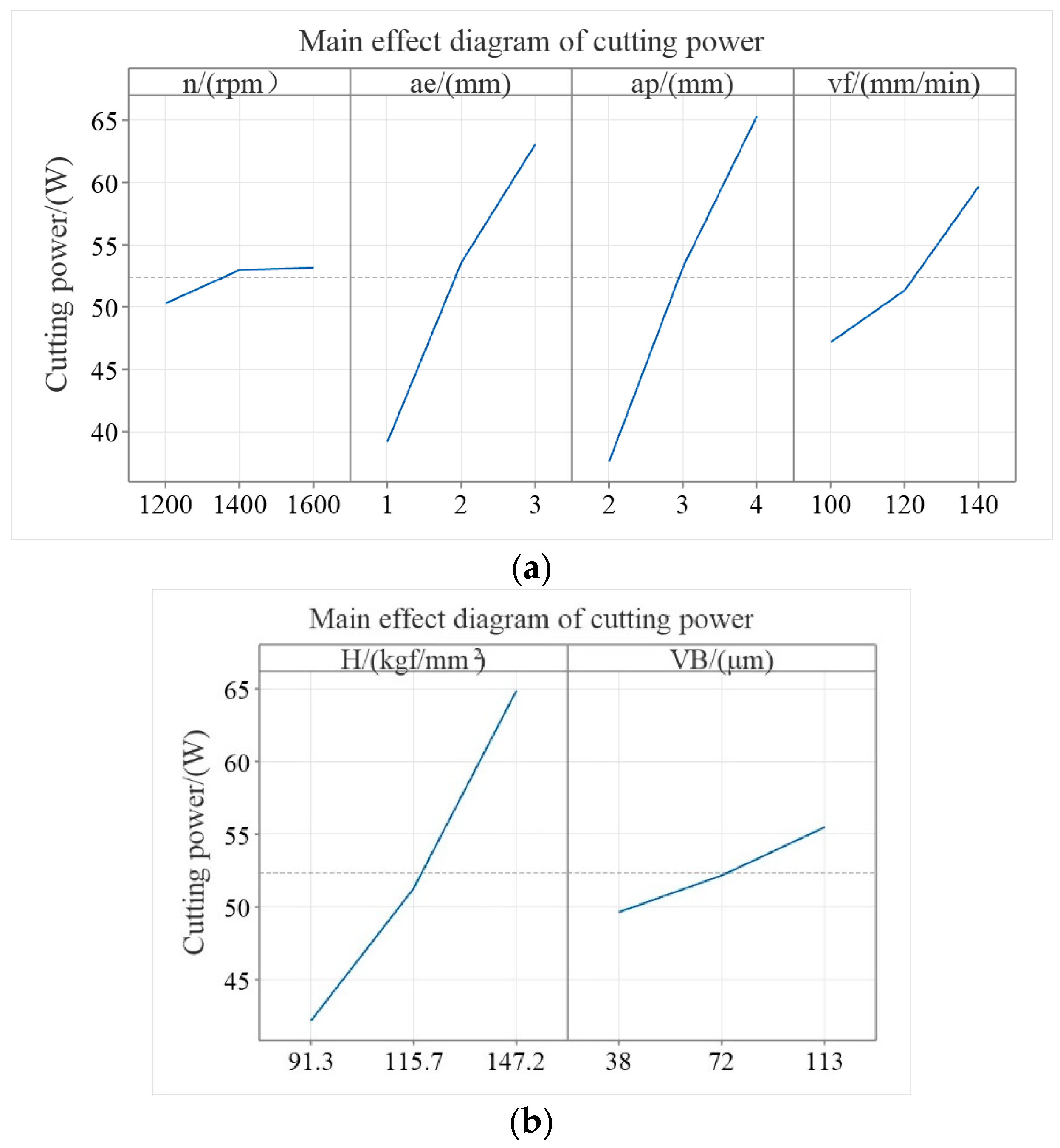
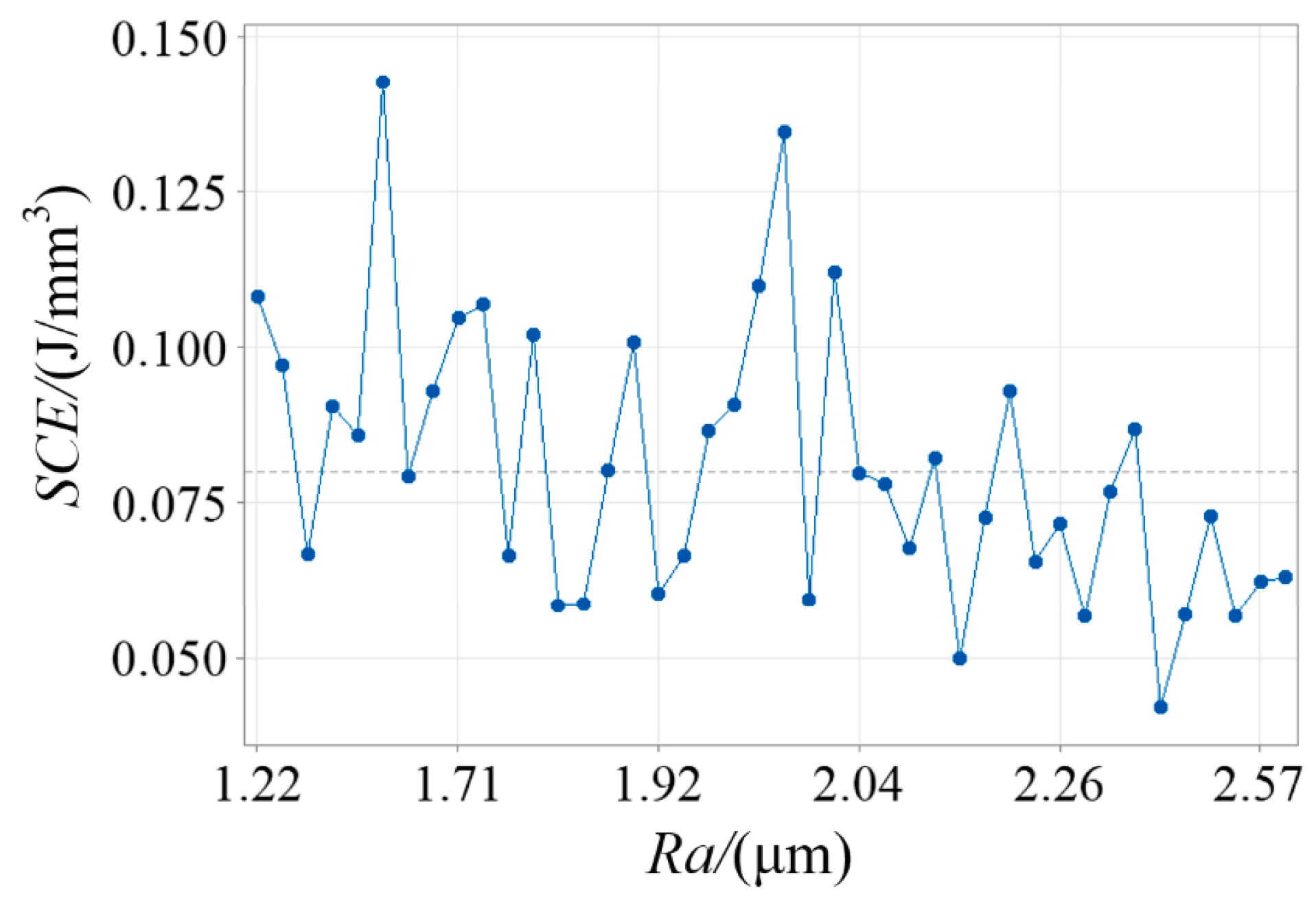
• The influence laws of cutting parameters, the hardness of workpiece material, and tool wear on machine power have been studied. The order of its influence from large to small is as follows: cutting depth, cutting width, material hardness, feed rate, tool wear, and spindle speed. As the surface roughness increases, the SCE generally tends to decrease.
• MOMRFO acquires the optimal machining parameters for minimizing energy consumption while guaranteeing machining quality. The comparison between before and after optimization reveals that SEC, MRR, and Ra have, respectively, increased by more than 44%, 53%, and 38%. It is demonstrated that the MOMRFO algorithm exhibits excellent optimization performance in the multi-objective optimization model developed in this paper and reduces the energy consumption of machine tools.

The cutting power model proposed in this study has a high prediction accuracy. However, due to the complexity of the energy flow of the machining process, the modeling process ignores the temperature of the chips. The cutting energy in the material removal process contains not only the plastic deformation energy and friction energy, but also the surface forming energy of the cutting material, elastic deformation energy, and the kinetic energy of the chips outflow. In future work, it will be necessary to further refine the study of the above issues. Meanwhile, this study is modeled for three-axis machine tools. Five-axis machine tools are required for workpieces with complex features such as curved surfaces. The study of energy consumption in 5-axis machines incorporates economic efficiency into the optimization objectives. Further reductions in energy consumption, improvements in machining quality, and improvements in economic efficiency represent the pathway to future development.

References

- IEA. Net Zero Roadmap: A Global Pathway to Keep the 1.5 °C Goal in Reach, IEA, Paris. 2023. Available online: https://www.iea.org/reports/net-zero-roadmap-a-global-pathway-to-keep-the-15-0c-goal-in-reach (accessed on 20 December 2023).
- IS0149551. 2014. Available online: http://www.iso.org/iso/catalogue_detail?csnumber=55294 (accessed on 20 December 2023).
- Zhou, L.; Li, J.; Li, F.; Meng, Q.; Li, J.; Xu, X. Energy consumption model and energy efficiency of machine tools: A comprehensive literature review. J. Clean. Prod. 2016, 112, 3721–3734. [Google Scholar] [CrossRef]
- Liu, F.; Wang, L.Q.; Liu, G.J. Content architecture and future trends of energy efficiency research on machining systems. J. Mech. Eng. 2013, 49, 87–94. [Google Scholar] [CrossRef]
- Shi, K.N.; Zhang, D.H.; Liu, N.; Wang, S.B.; Ren, J.X.; Wang, S.L. A novel energy consumption model for milling process considering tool wear progression. J. Clean. Prod. 2018, 184, 152–159. [Google Scholar] [CrossRef]
- Gutowski, T.; Dahmus, J.; Thiriez, A. Electrical energy requirements for manufacturing processes. In Proceedings of the 13th CIRP International Conference on Life Cycle Engineering, Leuven, Belgium, 31 May–2 June 2006; Volume 31, pp. 623–638. [Google Scholar]
- Gutowski, T.; Branham, M.; Dahmus, J.; Jones, A.; Thiriez, A. Thermodynamic analysis of resources used in manufacturing processes. Environ. Sci. Technol. 2009, 43, 1584–1590. [Google Scholar] [CrossRef] [PubMed]
- Kara, S.; Li, W. Unit process energy consumption models for material processes. CIRP Ann. Manuf. Technol. 2011, 61, 37–40. [Google Scholar] [CrossRef]
- Li, L.; Yan, J.H.; Xing, Z.W. Energy requirements evaluation of milling machines based on thermal equilibrium and empirical modeling. J. Clean. Prod. 2013, 52, 113–121. [Google Scholar] [CrossRef]
- Sihag, N.; Sangwan, K.S. A systematic literature review on machine tool energy consumption. J. Clean. Prod. 2020, 275, 123125. [Google Scholar] [CrossRef]
- Newman, S.T.; Nassehi, A.; Imani-Asrai, R.; Dhokia, V. Energy efficient process planning for CNC machining. CIRP J. Manuf. Sci. Technol. 2012, 5, 127–136. [Google Scholar] [CrossRef]
- Rodrigues, A.R.; Coelho, R.T. Influence of the tool edge geometry on specific cutting energy at high-speed cutting. J. Braz. Soc. Mech. Sci. Eng. 2007, 29, 279–283. [Google Scholar] [CrossRef]
- Pawar, S.S.; Bera, T.C.; Sangwan, K.S. Towards energy efficient milling of variable curved geometries. J. Manuf. Process 2023, 94, 451–497. [Google Scholar] [CrossRef]
- Shao, H.; Wang, H.L.; Zhao, X.M. A cutting power model for tool wear monitoring in milling. Int. Int. J. Mach. Tools Manuf. 2004, 44, 1503–1509. [Google Scholar] [CrossRef]
- Li, B.; Tian, X.T.; Zhang, M. Modeling and Multi-objective Optimization Method of Machine Tool Energy Consumption Considering Tool Wear. Int. J. Precis. Eng. Manuf.-Green Technol. 2021, 9, 127–141. [Google Scholar] [CrossRef]
- Liu, Z.Y.; Guo, Y.B.; Sealy, M.P.; Liu, Z.Q. Energy consumption and process sustainability of hard milling with tool wear progression. J. Mater. Process. Technol. 2016, 229, 305–312. [Google Scholar] [CrossRef]
- Li, C.B.; Wu, S.Q.; Yi, Q.; Zhao, X.K.; Cui, L.G. A cutting parameter energy-saving optimization method considering tool wear for multi-feature parts batch processing. Int. J. Adv. Manuf. Technol. 2022, 121, 4941–4960. [Google Scholar] [CrossRef]
- Bayoumi, A.E.; Yuicesan, G.; Hutton, D.V. On the closed form mechanistic modeling of milling: Specific cutting energy, torque, and power. J. Mater. Eng. Perform. 1994, 3, 151–158. [Google Scholar] [CrossRef]
- Pramanik, A.; Zhang, L.C.J.; Arsecularatne, A. Prediction of cutting forces in machining of metal matrix composites. Int. Int. J. Mach. Tools Manuf. 2006, 46, 1795–1803. [Google Scholar] [CrossRef]
- Wang, B.; Liu, Z.Q.; Cai, Y.K.; Song, Q.H.; Ren, X.P. Effects of tool angles and uncut chip thickness on consumption of plastic deformation energy during machining process. J. Manuf. Process 2023, 87, 123–132. [Google Scholar] [CrossRef]
- Tang, Z.; Huang, C.; Shi, Z.; Liu, H.; Chen, Z.; Li, B.; Niu, J.; Chen, Z. Modeling energy consumption inside cutting deformation zone to predict the stress distributions, temperature and microstructure by micro irreversible entropic thermodynamics. J. Manuf. Process 2023, 98, 357–370. [Google Scholar] [CrossRef]
- Guo, Y.S.; Loenders, J.; Duflou, J.; Lauwers, B. Optimization of energy consumption and surface quality in finish turning. Procedia CIRP. 2012, 1, 512–517. [Google Scholar] [CrossRef]
- Kant, G.; Sangwan, K.S. Prediction and optimization of machining parameters for minimizing power consumption and surface roughness in machining. J. Clean. Prod. 2014, 83, 151–164. [Google Scholar] [CrossRef]
- Chen, X.; Li, C.; Tang, Y.; Li, L.; Li, H. Energy efficient cutting parameter optimization. Front. Mech. Eng. 2021, 16, 221–248. [Google Scholar] [CrossRef]
- Chetan Ghosh, S.; Rao, P.V. Specific cutting energy modeling for turning nickel-based Nimonic 90 alloy under MQL condition. Int. J. Mech. Sci. 2018, 146, 25–38. [Google Scholar] [CrossRef]
- Guo, K.; Zhang, L.M. Multi-objective optimization for improved project management: Current status and future directions. Autom. Constr. 2022, 139, 104256. [Google Scholar] [CrossRef]
- Mirjalili, S.; Jangir, P.; Saremi, S. Multi-objective ant lion optimizer: A multi-objective optimization algorithm for solving engineering problems. Appl. Intell. 2017, 46, 79–95. [Google Scholar] [CrossRef]
- Verma, S.; Pant, M.; Snasel, V. A Comprehensive Review on NSGA-II for Multi-Objective Combinatorial Optimization Problems. IEEE Access 2021, 9, 57757–57791. [Google Scholar] [CrossRef]
- Zhang, X.Y.; Zheng, X.T.; Cheng, R. A competitive mechanism based multi-objective particle swarm optimizer with fast convergence. Inf. Sci. 2018, 427, 63–76. [Google Scholar] [CrossRef]
- Lu, C.; Liu, Q.; Zhang, B.; Yin, L. A Pareto-based hybrid iterated greedy algorithm for energy-efficient scheduling of distributed hybrid flowshop. Expert Syst. Appl. 2022, 204, 117555. [Google Scholar] [CrossRef]
- Moldovan, D.; Slowik, A. Energy consumption prediction of appliances using machine learning and multi-objective binary grey wolf optimization for feature selection. Appl. Soft Comput. 2021, 111, 107745. [Google Scholar] [CrossRef]
- Johnson, G.R.; Cook, W.H. Fracture characteristics of three metals subjected to various strains, strain rates, temperatures and pressures. Eng. Fract. Mech. 1985, 21, 31–48. [Google Scholar] [CrossRef]
- Khonengerg, M. Machining Science and Application. In Theory and Practice for Operation and Development of Machining Processes; Pergamon Press: Oxford, UK, 1966. [Google Scholar]
- MF, P. Contact Loads on Tool Interfaces; Mashinostroenie: Moscow, Russia, 1969.
- Özbek, O. Evaluation of Nano Fluids with Minimum Quantity Lubrication in Turning of Ni-Base Superalloy UDIMET720. Lubricants 2023, 11, 159. [Google Scholar] [CrossRef]
- Got, A.; Zouache, D.; Moussaoui, A. MOMRFO: Multi-objective Manta ray foraging optimizer for handling engineering design problems. Knowl.-Based Syst. 2022, 237, 107880. [Google Scholar] [CrossRef]
- Zhao, W.; Zhang, Z.; Wang, L. Manta ray foraging optimization: An effective bio-inspired optimizer for engineering applications. Eng. Appl. Artif. Intell. 2020, 87, 103300. [Google Scholar] [CrossRef]
Disclaimer/Publisher’s Note: The statements, opinions and data contained in all publications are solely those of the individual author(s) and contributor(s) and not of MDPI and/or the editor(s). MDPI and/or the editor(s) disclaim responsibility for any injury to people or property resulting from any ideas, methods, instructions or products referred to in the content. |
© 2024 by the authors. Licensee MDPI, Basel, Switzerland. This article is an open access article distributed under the terms and conditions of the Creative Commons Attribution (CC BY) license (https://creativecommons.org/licenses/by/4.0/).