Modeling and Characteristics of Airless Spray Film Formation

Abstract

Based on the computational fluid dynamics (CFD) theory, this paper proposes a film formation model and a numerical simulation method that can be used in thickness prediction of airless spraying robots. The spraying flow field and the film formation process in the airless spraying process were simulated by the Eulerian–Eulerian approach, and the airless spraying film formation model including the paint expansion model and the wall hitting model was established. To verify the correctness of the model, numerical simulations of static spraying and dynamic spraying were carried out on the plane and arc surfaces. The simulation results showed that the width of the spraying flow field on the far wall increased linearly with the longitudinal distance in the major-axis direction. The busbar spraying on the outer surface of the arc surface showed the similar characteristics to the plane in the major-axis direction. Besides, the annular spraying was similar to the plane spraying in the minor-axis direction, but the inner surface spraying was completely opposite. When spraying the outer surface, the film thickness increased with the increase of the inner diameter but was smaller than that of the plane spraying, while the inner surface spraying was completely opposite. In the spraying experiment, the plane dynamic spraying and the arc plane inner and outer surface translation spraying were selected for verification. The experimental results were in good agreement with the simulation results, indicating that the film formation model of airless spraying established in this paper is basically correct. As a result, this model can be used for thickness prediction of spraying robots.

1. Introduction

Airless spraying exhibits the advantages of good spraying surface quality, strong adhesion, high paint utilization rates, and high construction efficiency, which is widely used in the anticorrosion of large machinery and metal facilities and equipment [1]. The robot spraying process of airless spraying is mainly divided into four stages: designing a spraying robot based on a computer-aided design (CAD) model of the workpiece and a film formation model [2], obtaining the spraying operation trajectory through offline planning [3], spraying thickness simulation and robot joint trajectory generation [4], and spraying test verification and productive spraying. However, due to the lack of a reasonable airless spraying film formation model, the problems such as unsatisfactory spraying trajectory planning for complex surfaces, inaccurate numerical simulation of spraying thickness, and difficulty in controlling the quality of the coating film emerge, when the spraying robot operates [5]. Finding a reasonable airless spraying film formation model and then exploring the film formation characteristics of airless spraying has become a key problem to be solved urgently.

At present, there are few studies on the film formation model of airless spraying. Ye et al. [6] simulated the process of the paint hitting the bottom plate, proving that the viscosity and the speed of the paint are the key factors of film formation. However, they did not establish an effective airless spraying film formation model. By comparison, there are many studies on air spraying and electrostatic spraying which can provide reference owing to the fact that the differences between these spraying methods only lie in the different atomization ways [7].

The research on the film formation model is mainly based on the method of computational fluid dynamics (CFD) now. According to the different treatment methods of paint droplets, there are the Eulerian–Eulerian approach [8,9,10] and the Eulerian–Lagrangian approach [11]. The Eulerian–Lagrangian approach takes the mass, momentum, energy, and compositional exchange between discrete and continuous phases through the physical properties of individual droplets into account. Through the two-way coupling method, researchers considered the interaction between the two phases in the modeling [12,13,14,15]. Yang et al. [16] proposed a coating film-forming model based on the Euler–Lagrangian method and established a Rosin–Rammler atomization model. Zhou et al. [17] applied a coupling algorithm between Volume of Fluid and Lagrangian Particle Tracking (VOF–LPT) for spraying simulations. Venkatachalam et al. [18] used a standard k-Ω model to simulate the turbulent continuous phase flow and employed the discrete phase model to track the spray droplets. However, the calculation process ignores the gas volume displacement caused by the droplets, which affects the calculation accuracy. In contrast, Pandal et al. [19] regarded the droplets as the continuous phase by averaging the droplets in the time or space domain, which considered that the droplet phase and the air phase had mutual penetration in space. Both phases were processed in the Euler coordinate system. The calculation results are acceptable for engineering situations. Zhong et al. [20] adopted the VOF method and Shear Stress Transfer (SST) k-ω turbulence model to deeply understand the flow characteristics of the nozzle. Payri et al. [21] used the VOF approach to analyze the flow inside the nozzle and the first 2–5 mm of the spray. The Eulerian–Eulerian approach can completely explore the turbulent motion process of each phase, and the calculation results can show the detailed information on the spatial distribution of the droplet phase. A unified numerical method can be used for the two gas–liquid phases; in addition, the calculation amount is relatively small.

In this paper, a film formation model of airless spraying based on the Eulerian–Eulerian approach was proposed. Based on this model, the film formation characteristics of planes and arc planes were analyzed, and the film formation model was established according to the process of airless spraying. The numerical simulation setting method was introduced, and the characteristics of the spray flow field and the coating film were analyzed based on the CFD method. The results of the film morphology and the thickness of planes and arc surfaces sprayed by a spray gun were given to verify the method proposed in this paper.

2. Film Formation Model

2.1. Airless Spraying Process

Figure 1 shows a complete airless spraying process consists of a paint atomization process and a paint film formation process. The paint film formation process includes the expansion of the paint phase and the wall impact film formation process of the paint droplets. The atomization process is not the focus of this study. It can be considered that the paint is atomized when it is injected into the air from the nozzle, and only the atomization results are used as the initial and boundary conditions of the paint film formation process.

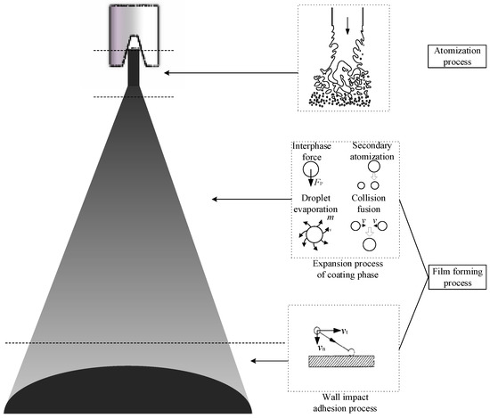
Figure 1. Airless spraying process [22].

The expansion process of the paint phase is a process in which the paint phase collides with the air phase and itself and gradually moves to the wall. It only takes 0.5 ms for the paint to shoot from the nozzle to the wall. Various components of the paint will volatilize into the air, but it can be considered that the components remain constant throughout the coating film formation process.

The wall impact adhesion process is that the paint droplets move to the surface of the workpiece and adhere to the surface to form a coating film. Due to the difference of the speed, collision angle, and particle size, there will be adhesion, rebound, stretch, breakage, and splashing, when the paint droplets move to the wall.

2.2. Paint Expansion Model

2.2.1. Two-Phase Flow Governing Equation

The time for the paint to reach the wall from the nozzle is extremely short, and the components and temperatures in the environment are basically constant. Therefore, the mass transfer and heat transfer phenomena are negligible in the modeling, and the Euler multiphase flow model [8] can be used to establish the conservation equation.

The governing equation for the paint droplet is shown as following:

$$\frac{d{u}_s}{dt}=\frac{g_x}{\rho }\left(\rho -{\rho }_s\right)+F_{D}u-F_D{u}_s+F_x,$$

(1)

where u is the velocity of the external air phase (m/s), u_s is the velocity of the paint droplet phase (m/s), ρ is the density of the external air phase (kg/m³), ρ_s is the density of the droplet phase (kg/m³), $\frac{g_x}{\rho }\left(\rho -{\rho }_s\right)$ is the unit net buoyancy of the paint, F_D is the drag force of the air relative to the paint droplet [23], and F_x is other acting forces.

The continuity equation is written as follow:

$$\frac{\partial }{\partial t}\left({\alpha }_l{\rho }_l\right)+\nabla \times \left({\alpha }_l{\rho }_l{\overrightarrow{v}}_l\right)=S_{{\alpha }_l}+{\displaystyle \sum _{l=1}^n\left({\dot{m}}_{gl}-{\dot{m}}_{lg}\right)},$$

(2)

where ${\dot{m}}_{gl}$ and ${\dot{m}}_{lg}$ are the masses transferred from the air phase to the paint phase and vice versa. Due to the two phases are incompatible with each other, the value here is 0; $S_{{\alpha }_l}$ is the quality of the source.

The momentum equation is shown as follow:

$$\frac{\partial }{\partial t}\left({\alpha }_g{\rho }_g{\overrightarrow{v}}_g\right)+\nabla \times \left({\alpha }_g{\rho }_g{\overrightarrow{v}}_g{\overrightarrow{v}}_g\right)=\nabla \times \overline{\overline{{\tau }_g}}-{\alpha }_g\nabla p+F_{d,g},$$

(3)

where p is the interphase acting force, F_d,g is the drag force, and $\overline{\overline{{\tau }_g}}$ is the pressure–strain tensor of the air phase.

For the modeling of surface tension, the Continuum Surface Stress Model (CSS) method was used to calculate the radius of curvature of the droplet surface, instead of the display method. Based on the capillary force model of surface stress, the anisotropic variable can be worked out. The surface stress tensor caused by surface tension is expressed as follows:

$$T=\sigma \left(I-\widehat{n}\otimes \widehat{n}\right)|\overrightarrow{n}|,$$

(4)

$$\overrightarrow{n}=\nabla \alpha ,$$

(5)

$$\widehat{n}=\frac{\overrightarrow{n}}{|\overrightarrow{n}|},$$

(6)

where I is the unit tensor, σ is the surface tension coefficient, $\otimes$ is the tensor product of the original normal vector and the transformed normal vector, α is the volume rate, and $\overrightarrow{n}$ is the volume rate gradient. The surface stress tensor can also be replaced with the following form:

$$T=\sigma \left(\left|\nabla \alpha \right|I-\frac{\nabla \alpha \otimes \nabla \alpha }{\left|\nabla \alpha \right|}\right).$$

(7)

The surface tension expressed by the CSS method can be expressed as:

$$F_{CSS}=\nabla \times T.$$

(8)

2.2.2. Turbulence Model

The turbulence model can be described as:

$$\begin{array}{ll}\frac{\partial }{\partial t}\left(\rho u_i\right)+\frac{\partial }{\partial x_j}\left(\rho u_i{u}_j\right)& =\left[\mu \left(\frac{\partial u_i}{\partial x_j}+\frac{\partial u_j}{\partial x_i}-{\delta }_{ij}\frac{2u_l}{3\partial x_l}\right)\right]\\ & +\frac{\partial }{\partial x_j}\left(-\rho \overline{u_i^{\prime }{u}_j^{\prime }}\right)-\frac{\partial p}{\partial x_i}\end{array},$$

(9)

where $-\rho \overline{u_i^{\prime }{u}_j^{\prime }}$ is the additional term of Reynolds stress due to turbulent flow. In order to close the momentum equation, the Reynolds stress term needs to be modeled. Compared with the Reynolds stress model (RSM), the viscous vortex model does not directly solve the Reynolds stress term but connects the Reynolds stress and the average velocity, which greatly improves the calculation efficiency. The equation is as follows:

$$\rho u_i^{\prime }{u}_j^{\prime }+\mu \left(\frac{\partial u_i}{\partial x_j}+\frac{\partial u_j}{\partial x_i}\right)=\frac{2{\delta }_{ij}}{3}\left(\rho k+{\mu }_t\frac{\partial u_i}{\partial x_j}\right),$$

(10)

where μ_t is the average kinetic acceleration viscosity of the entire turbulent flow, μ_i is the time-averaged velocity, and k is the average kinetic energy of the entire turbulent flow.

The Reynolds-averaged Navier–Stokes (RNG k-ε) Model in the viscous vortex model was chosen [24], which is mainly composed of the turbulent kinetic energy equation, namely the k equation, and the dissipation rate equation (the ε equation):

$$\frac{\partial }{\partial t}\left(\rho k\right)+\frac{\partial }{\partial x_i}\left(\rho k{u}_i\right)=\frac{\partial }{\partial x_j}\left({\alpha }_k{\mu }_{eff}\frac{\partial k}{\partial x_j}\right)+G_k+G_b+S_k-Y_k-\rho \epsilon ,$$

(11)

$$\frac{\partial }{\partial t}\left(\rho \epsilon \right)+\frac{\partial }{\partial x_i}\left(\rho \epsilon u_i\right)=\frac{\partial }{\partial x_j}\left({\alpha }_{\epsilon }{\mu }_{eff}\frac{\partial \epsilon }{\partial x_j}\right)+\frac{\epsilon }{k}{C}_{1\epsilon }{G}_k-\rho C_{2\epsilon }\frac{{\epsilon }^2}{k}+S_{\epsilon },$$

(12)

where G_k is the turbulent kinetic energy caused by the average velocity gradient, G_ε is the ε turbulent kinetic energy, Y_M is the divergence of the pulsatile expansion to the overall dissipation rate in compressible turbulence, S_k and S_ε are the custom source terms, ${\alpha }_k{\mu }_{eff}$ and ${\alpha }_{\epsilon }{\mu }_{eff}$ represent the effective diffusion coefficients of k and ε, respectively, and σ_k and σ_ε are the Prandtl numbers of k and ε, respectively.

2.3. Wall Impact Model

2.3.1. Near-Wall Model

The difference of wall conditions is the main reason for the variations in average vorticity and turbulence, so accurately representing the flow in the near-wall region can better reflect the coating film formation. The standard wall function method was chosen to describe the flow near the wall, and the momentum equation was combined with the turbulent kinetic energy and the dissipation rate in the near-wall mesh. A unified wall surface function was chosen to relate the bottom region affected by viscosity to the turbulence logarithm equation, which can be applied to the calculation of the entire near-wall flow. The dimensionless velocity in the mean velocity region is shown as following:

$$U^{*}=\frac{1}{\kappa }\ln \left(E{y}^{*}\right),$$

(13)

$$U^{*}\equiv \frac{U_N{C}_{\mu }^{1/4}{k}_N^{1/2}}{{\tau }_w/\rho },$$

(14)

where U* is the dimensionless velocity, U_N is the average flow velocity at point N, k_N is the turbulent kinetic energy at point N, y_N is the distance from point N to the wall, μ is the dynamic viscosity of the fluid, $\kappa$ is the Karman constant (0.4187), E is the empirical constant (the value is usually 9.793), and y* is the dimensionless distance to the wall and written as:

$$y^{*}\equiv \frac{\rho C_{\mu }^{1/4}{k}_P^{1/2}{y}_P}{\mu }.$$

(15)

In the standard wall function method, for y* > 11.225, it indicates that point N is in the completely turbulent region at that time, and the logarithmic law applies. Otherwise, the point N is in the viscous bottom layer and the laminar flow stress–strain relationship applies:

$$y^{*}=U^{*}.$$

(16)

2.3.2. Liquid Film Model

By the CFD method, Mirko et al. [25] proved that after the paint droplets reach the surface of the workpiece, the friction caused by the high viscosity of the droplets dissipates its inertia. When the liquid flakes reach their maximum diameter, the impact stops and almost all remain on the wall. Therefore, it is assumed in this paper that all paint droplets reaching the surface of the workpiece participate in the formation of the coating film. The Eulerian Wall Film (EWF) model [26] was chosen to establish the adhesive film formation model.

The mass conservation equation of the liquid film can be expressed as:

$$\frac{\partial {\rho }_{l}h}{\partial t}+{\nabla }_s\times \left({\rho }_{l}h{\overrightarrow{V}}_l\right)={\dot{m}}_s,$$

(17)

where ρ is the paint density, h is the liquid film height, ∇_s is the surface gradient operator, $\overrightarrow{V}$ is the average film velocity, and ${\dot{m}}_s$ is the mass source per unit surface area caused by droplet deposition, film separation, or peeling and phase transition.

The momentum equation can be expressed as:

$$\frac{\partial {\rho }_{l}h{\overrightarrow{V}}_l}{\partial t}+{\nabla }_s\times \left({\rho }_{l}h{\overrightarrow{V}}_l{\overrightarrow{V}}_l+{\overrightarrow{D}}_V\right)=-h{\nabla }_s{P}_L+{\rho }_{l}h{\overrightarrow{g}}_{\tau }+\frac{3}{2}{\overrightarrow{\tau }}_{fs}-\frac{3}{h}{\mu }_l{\overrightarrow{V}}_l+{\dot{\overrightarrow{q}}}_s+{\overrightarrow{\tau }}_{\theta w}$$

(18)

$$P_L=P_{gas}+P_h+P_{\sigma },P_h=-\rho \left(\overrightarrow{n}\times \overrightarrow{g}\right)h,P_{\sigma }=-\sigma {\nabla }_s\times \left({\nabla }_{s}h\right).$$

(19)

The left side of Equation (18) represents the instantaneous term and the convection term. The first term on the right side of Equation (18) represents the air pressure, the normal component of gravity perpendicular to the workpiece surface, and the coupling effect of surface tension on the wall surface. The second term represents the tangent of gravity along the workpiece surface. The third and fourth terms represent the net viscous shear force at the interface between the gas and the film. The fifth term represents the quantity related to the deposition and diffusion of droplets. The sixth term represents the surface tension caused by the liquid film and contact angle-induced surface forces. Equation (19) is the complement of Equation (18).

In the multiphase flow calculation, the mass phase and the momentum phase of the paint phase were shifted out of the conservation equation of the air-paint spray flow field. Besides, they were added to the mass and momentum equations of the liquid film on the workpiece surface as the source terms.

The quality source term is written as:

$${\dot{m}}_s={\alpha }_l{\rho }_l{v}_l{}_n.$$

(20)

The momentum source term is described as:

$${\dot{q}}_s={\dot{m}}_s{v}_l.$$

(21)

3. Numerical Simulations

3.1. Nozzle Geometry Model

The model number of the nozzle was Graco-525 (Beida Mechanical Engineering Co., Ltd., Guangzhou, China). As is shown in Figure 2a, the fan nozzle was mainly composed of a nozzle paint channel and a duckbill. The diameter of the nozzle outlet was 0.025 in (0.635 mm). There was a V-shaped wall near the nozzle outlet, and the outlet shape was oval. According to the actual shape of the nozzle, the geometric model is shown in Figure 2b. The short-axis direction, that is, the radial direction perpendicular to the V-shaped wall surface was set as the x-axis; the long-axis direction, that is, the radial direction of the V-shaped wall surface, was set as the y-axis.

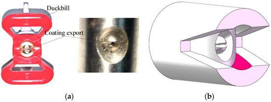
Figure 2. Nozzle geometric model. (a) Picture of the nozzle. (b) Nozzle model.

3.2. Computational Domain and Meshing

The established plane and arc spraying calculation domains are shown in Figure 3 and Figure 4, respectively.

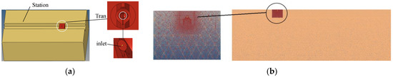
Figure 3. Computational domain and meshing of the plane spraying. (a) Computational domain. (b) Meshing.

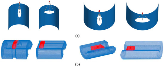
Figure 4. Computational domain and mesh division of the arc surface spraying. (a) Computational domain. (b) Meshing.

3.3. Parameter Setting

The basic parameter settings of the numerical simulation are shown in Table 1. The environment in the computational domain was set to 1 atm, and the time type was transient. The first phase was set to the air phase, and the second phase was the paint phase. The inlet was set at the outlet of the nozzle, and the paint inlet was directly connected to the outside atmosphere. Therefore, the pressure inlet was changed to the mass flow inlet.

Table 1. The basic parameter settings of the numerical simulation.

Parameters	Values
Density	1320 kg/m3
Dynamic viscosity	0.275 kg/(m·s)
Surface tension coefficient	0.036 N/m
Spraying distance	400 mm
Mass flow rate	0.0787 g/s
	0.103 kg/s
	0.125 kg/s
Turbulence intensity	5%
Hydraulic diameter	0.6 mm
Maximum time step	700
Spraying speed	0.15 m/s

The dynamic spraying settings were the same as those of the plane spraying, using a sliding grid to define the speed of the nozzle along the x-axis direction. The maximum time step was set to 3000, and the dynamic spraying time and linear spraying distance were 3 s and 4.5 m, respectively.

The coupled algorithm was used for the coupling equations of pressure and velocity in static spraying and dynamic spraying. The gradient of the empty grid was discretized by the least squares cell-based method. The momentum, the volume fraction turbulent kinetic energy, and the turbulent dissipation rate were discretized by first-order upwind. The time term in the transient equation was discretized by first-order implicit.

4. Characteristics of the Spray Flow Field

4.1. Division of the Spray Flow Field

According to the flow characteristics of the jet, the airless spray flow field was divided into the free jet region, the impingement region, and the wall flow region, as is shown in Figure 5. There was no difference between the paint and the free jet in the free jet zone. In the impact zone, the paint hit the wall vertically, and the paint flow was obviously bent, forming a great pressure gradient and a tangential velocity along the wall. The paint almost became a horizontal flow and then entered the wall flow zone.

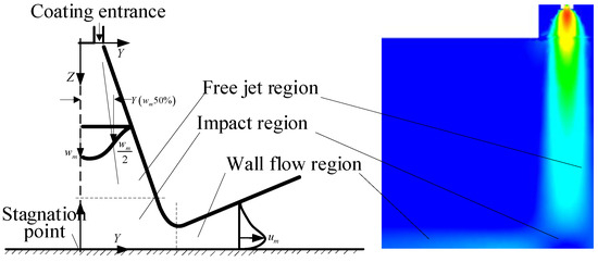
Figure 5. Division of the spray flow field.

The half-value width Y (50%) of the velocity is not only an important indicator of the spray velocity along the vertical axis, but also an important indicator to reflect the horizontal expansion of the spray range and the change of the spray width with the vertical axis. The Y (50%) distribution on the central vertical axis is shown in Figure 6.

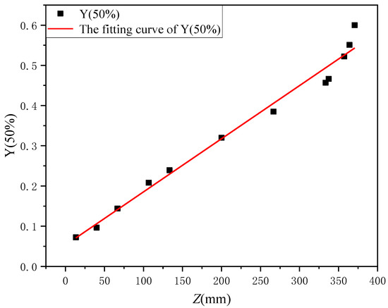
Figure 6. The relationship between the half-value width of the speed and the z-axis.

It can be found from Figure 6 that within 370 mm, the Y (50%) was basically linear with the z-axis and it increased with the z-axis distance. The slope was 1.36, and the corresponding spray cone angle was about 53.67°. However, when the spraying distance was greater than 370 mm, the Y (50%) and the z-axis cannot be linearly related. The reason is that the paint phase collided with the wall surface near the wall and the tangential velocity along the wall was obtained. Therefore, 370 mm can be regarded as the boundary between the near-wall flow field and the far-wall flow field, that is, the region of 0–370 mm from the entrance was the free jet area and the region of 370–400 mm was the impact area and the wall flow area.

This paper mainly studies the characteristics of the near-wall flow field. The coordinate system shown in Figure 7 was established in the near-wall flow field. The projection point from the nozzle center point to the wall is the coordinate origin, the direction of the short axis of the spray is the x-axis, the direction of the long axis of the spray is the y-axis, and the direction from the origin to the nozzle center point is the z-axis.

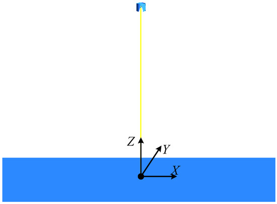
Figure 7. Coordinate system of the near-wall flow field.

4.2. Velocity Distribution Characteristics

The contours of the velocity distribution in the spray flow field are shown in Figure 8. Each figure shows the long-axis direction on the left and the short-axis direction on the right. It can be seen from the figure that the width of the spray flow field in the long-axis direction was wider than that in the short-axis direction. This phenomenon is mainly due to the following two reasons. One is the oval shape of the paint inlet, namely, the large width on the long axis and the small width on the short axis. The other is the influence of the wall near the nozzle outlet. The V-shaped walls on both sides of the nozzle outlet in the short-axis direction hindered the expansion of the paint phase velocity to the short-axis direction.

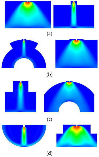
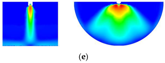
Figure 8. Contours of the spraying flow field velocity distribution. (a) Flat spraying flow field. (b) Spraying flow field of the busbar on the outer surface of the arc surface. (c) Circumferential spraying flow field on outer surface of the arc surface. (d) Spraying flow field of the busbar on the inner surface of the arc surface. (e) Circumferential spraying flow field on the inner surface of the arc surface.

The lateral velocity and the longitudinal velocity near the wall affected the film formation area and the film formation thickness, respectively. The velocity distributions of each cross-section and longitudinal section near the wall are shown in Figure 9.

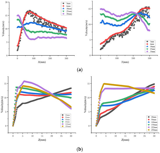
Figure 9. Velocity distributions. (a) Cross-sectional velocity. (b) Longitudinal-section velocity.

There was a point where the velocities coincided in the figure. On the left side of the point, the velocity gradient was distributed along the cross-section, but the reverse velocity gradient was distributed along the longitudinal section; the right side was the opposite distribution. According to the above analysis, the near-wall flow field was divided into four regions according to the velocity intersection in Figure 9. As is shown in Figure 10, the velocity gradient in zone I was upward and inward, the velocity gradient in zone II was downward and inward, the velocity gradient was upward and outward in zone III, and the velocity gradient was downward and outward in zone IV.

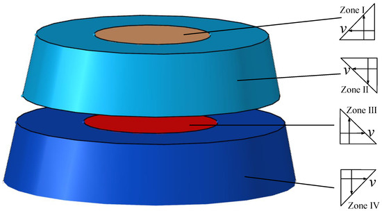
Figure 10. Division of the flow field near the wall.

4.3. Pressure Distribution Characteristics

Static spraying was carried out on the plane spraying and the arc surface with an inner diameter of 323.9 mm, in which the nozzle was located at the center of the arc when the inner surface was sprayed. The pressure distributions near the wall are shown in Figure 11 and Figure 12. Figure 11a–e shows the contours of the pressure distributions near the wall with different surfaces and directions. It can be seen from the figures that the shape of pressure distribution of the circumferential spraying pressure on the outer surface was a flat round rectangle. The pressure distribution contours obtained by the other three spraying were similar to those of the plane spraying, presenting a narrow and long round rectangle.

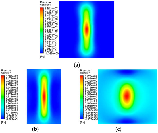
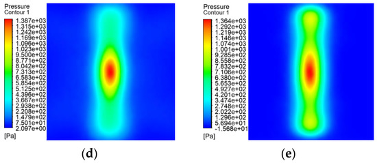
Figure 11. Distributions of the pressure near the wall. (a) Plane spraying pressure. (b) Outer surface busbar spraying pressure. (c) Circumferential spraying pressure on the outer surface. (d) Inner surface busbar spraying pressure. (e) Circumferential spraying pressure on the inner surface.

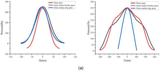
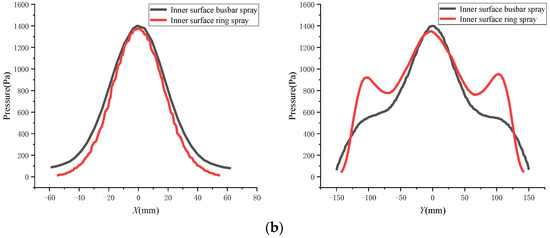
Figure 12. Pressure distributions near the wall. (a) Plane spraying and outer surface spraying pressures. (b) Inner surface spraying pressure.

Figure 12 shows the pressure distributions on the outer surface and the inner surface of the plane and the arc surface, respectively. The left was the short-axis distribution, and the right was the long-axis distribution. It can be seen from the figure that the pressure distribution of the inner surface was significantly higher than that of the outer surface and the plane, which was mainly caused by the semi-closed characteristic of the inner surface. In addition, the spraying distance of the inner surface was its radius, which was smaller than the distance of 400 mm sprayed on the plane and the outer surface, forming a high-pressure distribution. When spraying on the outer surface, the busbar spraying showed a similar pressure distribution characteristic to the plane in the long axis. Meanwhile, the circumferential spraying showed a similar pressure distribution characteristic to the plane in the short-axis direction. When spraying on the inner surface, the pressure distribution of the busbar spray was similar to that of the annular spraying in the direction of the short axis, and the overall variation trend was similar to that of the plane. In the direction of the long axis, the difference between the busbar spraying and the circumferential spraying was large, which was mainly manifested in the secondary pressure center (±100 mm) during the circumferential spraying.

5. Coating Film Characteristics

5.1. Characteristics of the Static Spraying Coating Film

Under the spraying pressure of 20 MPa, the coating film distribution of five spraying methods are shown in Figure 13a–e. It can be seen from the figure that the arc surface coating film was different from the flat coating film. The width of the outer surface busbar spraying in the short axis direction was smaller than that of the circumferential spraying and larger in the long-axis direction. The spraying trend of the inner surface was completely opposite to that of the outer surface.

Figure 13. Film thickness of the static spraying. (a) Plane spraying. (b) Outer surface busbar spraying. (c) Circumferential spraying on the outer surface. (d) Spraying on the inner surface busbar. (e) Circumferential spraying on the inner surface.

The changes of the coating film thickness under the plane spraying distances of 300, 400, and 500 mm are shown in Figure 14. The changes of the coating film thickness under the plane spraying pressures of 10, 15, and 20 MPa are shown in Figure 15. The short-axis direction is shown in the left figure, and the long-axis direction is shown in the right figure.

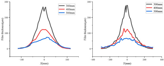
Figure 14. Film thicknesses at different spraying distances.

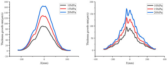
Figure 15. Growth rates of coating films under different spraying pressures.

It can be seen from the figures above that when the spraying distance increased by 100 mm, the film thickness in the impact zone decreased by about 50%. In the wall flow area out of the x-axis (±50 mm) and the y-axis (±100 mm), the film thickness did not change significantly with the increase of the spraying distance. When the pressure increased by 5 MPa, the film thickness growth rate increased by about 37 μm/s, and the coating film area also gradually increased. Meanwhile, the difference of the film thickness between the double peak and the origin became larger, but its location was independent of the pressure.

5.2. Dynamic Coating Characteristics

The same settings of the dynamic spraying were selected as those of the flat spraying, with the moving speed being 0.15 m/s. When spraying the arc surface, the spraying methods were divided into rotary spraying and translational spraying in order to obtain a larger coating range. Different inner diameters of arcs were converted into angular velocities equivalent to linear velocities for spraying. The results of the dynamic spray coating are shown in Figure 16.

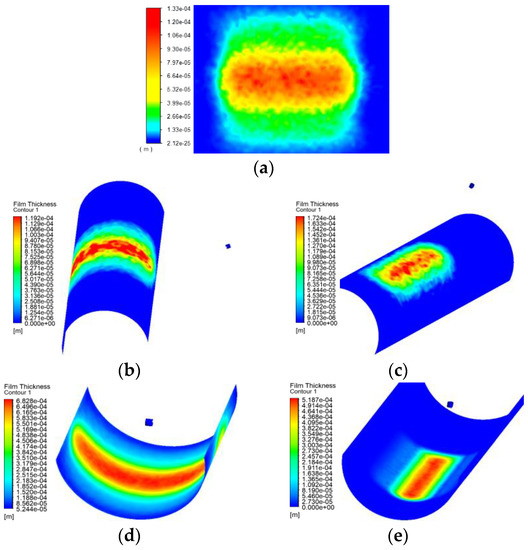
Figure 16. Coating film distributions of the dynamic spraying. (a) Plane spraying. (b) Outer surface busbar spraying. (c) Circumferential spraying on the outer surface. (d) Inner surface busbar spraying. (e) Circumferential spraying on the inner surface.

During dynamic spraying, the long-axis direction of the spray flow field moved along the short-axis direction, so this paper mainly studies the dynamic coating characteristics in the long-axis direction. Under the same linear velocity, the dynamic coating thickness distributions along the long axis are shown in Figure 17.

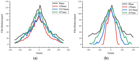
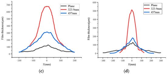
Figure 17. Film thickness distributions of the dynamic spraying. (a) Rotary spraying on the outer surface. (b) Outer surface translation spraying. (c) Rotary spraying on the inner surface. (d) Translation spraying on the inner surface.

As is shown in the figure above, the larger the inner diameter of the outer surface of the arc, the thicker the dynamic coating film. The thickness of the dynamic spray coating on the outer surface was smaller than that of the flat surface. The larger the inner surface diameter, the thinner the dynamic spraying film thickness. The film thickness on the inner surface was larger than that on the plane.

Under the spraying pressure of 20 MPa, the dynamic spraying was performed on the plane at 400 mm at the moving speeds of 0.1, 0.15, and 0.2 m/s separately. In order to ensure the same spraying distance, the spraying time was set to 4.5, 3, and 2.25 s separately. The corresponding coating film thickness distributions are shown in Figure 18.

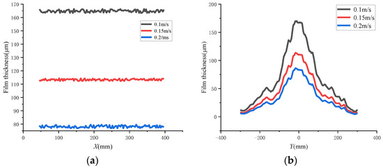
Figure 18. Film thickness distributions at different spraying speeds. (a) The film thickness of movement of the spray gun axis. (b) Axle wire film thickness distribution of the y-axis.

The film thickness decreased with the increasing spray speed, because a faster spray speed resulted in a slower paint deposition at each point. Taking the half-value thickness of the central film thickness as the effective thickness, the maximum film thickness was 167 μm at the spraying speed of 0.1 m/s. When the speed increased to 0.15 m/s, the thickness decreased to 110.2 μm and the maximum film thickness decreased by 34.1%. When the speed continued to increase to 0.2 m/s, the maximum film thickness was 83.2 μm, which decreased by 25% compared to that of the spraying speed of 0.15 m/s. It can be seen that the film thickness did not change linearly with the spraying speed. A too high spraying speed was of little significance in production, which led to poor film quality and uniformity. When the spraying speed was doubled, the film thickness became 0.67–0.75 times that the original thickness.

6. Experimental Validations

In order to verify the reliability of the numerical simulation results, static and dynamic spraying experiments were carried out on the plane and arc surfaces, respectively. The vertical distance between the spray gun and the workpiece surface was kept unchanged during static spraying. During dynamic spraying, the trajectory of the spraying robot was consistent with the motion situation of the numerical simulation. The coating film morphology and thickness were compared and analyzed as follows.

6.1. Coating Film Morphology Verification

The GB-Q235 steel plate (commonly used in construction and machinery industries; Jingshou Iron & Steel Trading Co., Ltd., Tianjin, China) was selected as the workpiece to be sprayed. The dynamic spraying was carried out under a linear speed of 0.15 m/s, a spraying pressure of 20 MPa, and a spraying distance of 400 mm. The coating films on the workpiece surface with plane spraying and arc surface translation spraying are shown in Figure 19 and Figure 20, respectively. The left of Figure 20 shows the outer surface spraying, and the right showed the inner surface spraying. As is seen from the figures, the gloss of the film was high and no obvious particle bulge, wrinkle, needle eye, and bubble on the film surface were observed. The coating film of the experiment was highly consistent with the results of the numerical simulation, which proved that the film formation model of airless spraying was basically correct.

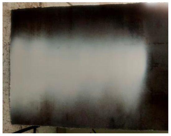
Figure 19. Plane dynamic spraying coating film.

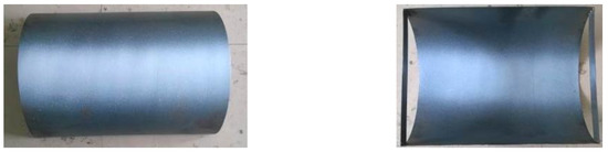
Figure 20. Dynamic spraying coating film distribution.

6.2. Verification of the Film Thickness

A number of points were selected on the center line of the long axis of the film obtained in the experiment. Combined with the numerical simulation results, the film thickness distributions of the experiment and the numerical simulation are shown in Figure 21. The corresponding error comparison is shown in Table 2.

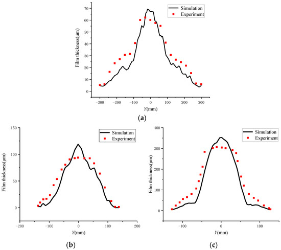
Figure 21. Dynamic spraying film thickness. (a) Plane spraying. (b) Outer surface translation spraying. (c) Inner surface translation spraying.

Table 2. Comparison of film thickness.

Spraying Method	Maximum Error (μm)	Average Error (μm)
Plane spraying	9.1	4.1
Outer surface translation spraying	21.8	9.7
Inner surface translation spraying	49.1	28.0

It can be seen that the numerical simulation results were in good agreement with the experiment results, which proved the correctness of the established film formation model. In the middle part of the coating film, the film thickness obtained in the experiment was lower than the simulation results but slightly higher than that in the simulation in the edge part. This is mainly because of the influence of the surface tension of the paint during the drying process. On the other hand, with the volatilization of the liquid components in the paint, the paint gradually flowed from the part with a high film thickness to the part with a low film thickness, resulting in the film thickness obtained in the experiment lower than that of the simulation results in the middle part. The maximum error and the average error were both less than 10 μm in the static spraying and were both less than 50 μm in the dynamic spraying. The average errors were 5.9%, 8.1%, and 7.7% for the plane, outer surface translation, and inner surface translation sprayings, respectively.

7. Conclusions

For the airless spraying process, the film formation model of airless spraying was established and solved based on the CFD method, and the film formation characteristics were summarized through the numerical simulation of the plane and the arc surface. The main conclusions are as follows:

(1)

According to the physical process of airless spraying, a film formation model of airless spraying including the paint expansion model and the wall impact model was established. The experiments verified the correctness of the film formation model.

(2)

In the outer surface spraying, the short-axis direction of the busbar spraying and the long-axis direction of the circumferential spraying showed similar pressure distribution characteristics to those of the plane spraying. In the inner surface spraying, the variation trend of the busbar spraying in the direction of the short axis was similar to that of the circumferential spraying. The circumferential spraying appeared a secondary pressure center in the long-axis direction.

(3)

When spraying the outer surface, the width in the long axis direction of the busbar spraying was larger than that of the circumferential spraying but smaller than that of the circumferential spraying in the short-axis direction. The characteristics of the inner surface spraying were completely opposite compared to those of the outer surface spraying. During the static spraying, the film thickness growth rate and the coating area increased with the increase of the spraying pressure and the deceasing of the spraying distance. During the dynamic spraying, the larger the diameter of the arc surface, the larger the thickness of the outer surface film and the smaller the thickness of the inner surface film.

References

- Cowlard, T. Airless Spraying. Trans. IMF 2017, 34, 420–426. [Google Scholar] [CrossRef]
- Zhang, Y.; Li, W.; Zhang, C.; Liao, H.; Zhang, Y.; Deng, S. A spherical surface coating thickness model for a robotized thermal spray system. Robot. Comput. Integr. Manuf. 2019, 59, 297–304. [Google Scholar] [CrossRef]
- Zhou, Y.; Ma, S.; Li, A.; Yang, L. Path planning for spray painting robot of horns surfaces in ship manufacturing. IOP Conf. Ser. Mater. Sci. Eng. 2019, 521, 012015. [Google Scholar] [CrossRef]
- Guan, L.; Chen, L. Trajectory planning method based on transitional segment optimization of spray painting robot on complex free surface. Ind. Robot. 2019, 46, 31–43. [Google Scholar] [CrossRef]
- Chen, W.; Chen, Y.; Zhang, W.; He, S.; Li, B.; Jiang, J. Paint thickness simulation for robotic painting of curved surfaces based on Euler–Euler approach. J. Braz. Soc. Mech. Sci. Eng. 2019, 41, 199. [Google Scholar] [CrossRef]
- Ye, Q.; Domnick, J. Analysis of droplet impingement of different atomizers used in spray coating processes. J. Coat. Technol. Res. 2017, 14, 1–10. [Google Scholar] [CrossRef]
- Eric, R.; John, L.; Josh, C. How to select an airless sprayer: Power sources. J. Prot. Coat. Linings 2019, 36, 24–26. [Google Scholar]
- Chen, Y.; Chen, W.Z.; He, S.W.; Pan, H.W.; Li, B.; Zhang, W.M. Spray flow characteristics of painting cylindrical surface with a pneumatic atomizer. China Surf. Eng. 2017, 30, 122–131. [Google Scholar]
- Chen, Y.; Chen, S.M.; Chen, W.Z.; Hu, J.; Jiang, J. An atomization model of air spraying using the volume-of-fluid method and large eddy simulation. Coatings 2021, 11, 1400. [Google Scholar] [CrossRef]
- Chen, S.; Chen, W.; Chen, Y.; Jiang, J.; Wu, Z.; Zhou, S. Research on film-forming characteristics and mechanism of painting V-shaped surfaces. Coatings 2022, 12, 658. [Google Scholar] [CrossRef]
- Ye, Q.; Karlheinz, P. Numerical and experimental investigation on the spray coating process using a pneumatic atomizer: Influences of operating conditions and target geometries. Coatings 2017, 7, 13. [Google Scholar] [CrossRef] [Green Version]
- Yu, Y.; Li, Y.; Jiang, M.; Zhou, Q. Meso scale drag model designed for coarse grid Eulerian-Lagrangian simulation of gas solid flows. Chem. Eng. Sci. 2020, 223, 115747. [Google Scholar] [CrossRef]
- Mergheni, M.A.; Ticha, H.B.; Sautet, J.C.; Nasrallah, S.B. Interaction particle turbulence in dispersed two phase flows using the eulerian-lagrangian approach. Int. J. Fluid Mech. Res. 2008, 35, 273–286. [Google Scholar] [CrossRef]
- Gu, J.; Shao, Y.; Liu, X.; Zhong, W.; Yu, A. Modelling of particle flow in a dual circulation fluidized bed by a Eulerian-Lagrangian approach. Chem. Eng. Sci. 2018, 192, 619–633. [Google Scholar] [CrossRef]
- Josef, A.; Jk, B.; Ss, B.; Radl, S. Coarse graining Euler Lagrange simulations of cohesive particle fluidization Science Direct. Powder Technol. 2020, 364, 167–182. [Google Scholar]
- Yang, G.; Chen, Y.; Chen, S.M.; Zhang, F. Modeling of Film Formation in Airless Spray. In Proceedings of the 2021 2nd International Conference on Modeling, Big Data Analytics and Simulation (MBDAS2021), Shenzhen, China, 14–15 November 2021. [Google Scholar]
- Zhou, W.; Xu, X.; Yang, Q.; Zhao, R.; Jin, Y. Experimental and numerical investigations on the spray characteristics of liquid-gas pintle injector. Aerosp. Sci. Technol. 2022, 121, 107354. [Google Scholar] [CrossRef]
- Venkatachalam, P.; Sahu, S.; Anupindi, K. Numerical investigation on the role of a mixer on spray impingement and mixing in channel cross-stream airflow. Phys. Fluids 2022, 34, 033316. [Google Scholar] [CrossRef]
- Pandal, A.; García Oliver, J.M.; Novella, R.; Pastor, J.M. A computational analysis of local flow for reacting Diesel sprays by means of an Eulerian CFD model. Int. J. Multiph. Flow 2018, 99, 257–272. [Google Scholar] [CrossRef] [Green Version]
- Zhong, J.; Dai, Y.; Liang, C.; Zhu, X.; Xu, L. CFD investigation of air-oil two-phase flow in oil jet nozzle. Proc. Inst. Mech. Eng. Part C J. Mech. Eng. Sci. 2022. [Google Scholar] [CrossRef]
- Payri, R.; Gimeno, J.; Marti-Aldaravi, P.; Martinez, M. Transient nozzle flow analysis and near field characterization of gasoline direct fuel injector using Large Eddy Simulation. Int. J. Multiph. Flow 2022, 148, 103920. [Google Scholar] [CrossRef]
- Chen, Y.; Chen, W.Z.; Li, B.; Zhang, G.; Zhang, W. Paint thickness simulation for painting robot trajectory planning: A review. Ind. Robot. -Int. J. Robot. Res. Appl. 2017, 44, 629–638. [Google Scholar] [CrossRef]
- Sazhin, S. Droplets and Sprays; Springer: London, UK, 2014. [Google Scholar]
- Spalding, B. The numerical computation of turbulent flows. Comput. Methods Appl. Mech. Eng. 1974, 103, 269–289. [Google Scholar]
- Mirko, G.; Marco, V.; Giancarlo, B. CFD modeling of a spray deposition process of paint. Macromol. Symp. 2002, 187, 719–730. [Google Scholar]
- O’Rourke, P.J.; Amsden, A.A. A Particle Numerical Model for Wall Film Dynamics in Port-Injected Engines. Off. Sci. Tech. Inf. Tech. Rep. 1996, 1, 961961. [Google Scholar]
Publisher’s Note: MDPI stays neutral with regard to jurisdictional claims in published maps and institutional affiliations. |
© 2022 by the authors. Licensee MDPI, Basel, Switzerland. This article is an open access article distributed under the terms and conditions of the Creative Commons Attribution (CC BY) license (https://creativecommons.org/licenses/by/4.0/).