Methodology for Predicting Geochemical Anomalies Using Preprocessing of Input Geological Data and Dual Application of a Multilayer Perceptron

Abstract

The increasing need for accurate prediction of geochemical anomalies requires methods capable of capturing complex spatial patterns that traditional approaches often fail to represent adequately. For N datasets of the form (X_i,Y_i) representing the geographic coordinates of sampling points and C_i denoting the geochemical measurement, training multilayer perceptrons (MLPs) presents a challenge. The low informativeness of the input features and their weak correlation with the target variable result in excessively simplified predictions. Analysis of a baseline model trained only on geographic coordinates showed that, while the loss function converges rapidly, the resulting values become overly “compressed” and fail to reflect the actual concentration range. To address this, a preprocessing method based on anisotropy was developed to enhance the correlation between input and output variables. This approach constructs, for each prediction point, a structured informational model that incorporates the direction and magnitude of spatial variability through sectoral and radial partitioning of the nearest sampling data. The transformed features are then used in a dual-MLP architecture, where the first network produces sectoral estimates, and the second aggregates them into the final prediction. The results show that anisotropic feature transformation significantly improves neural network prediction capabilities in geochemical analysis.

1. Introduction

In recent decades, global consumption of mineral raw materials has steadily increased. Alongside quantitative growth, the diversity of utilized mineral resources has expanded significantly, with new types of mineral commodities continuously being introduced into industrial practice. These resources increasingly form the foundation of technological progress and innovative development in the global economy. Under such conditions, the importance of scientifically grounded forecasting aimed at the discovery of new mineral deposits has grown substantially. This trend necessitates the continuous improvement of exploration methodologies and the adoption of advanced technologies to enhance the efficiency and reliability of modern predictive and prospecting approaches.

One of the most rapidly developing technological directions in addressing problems related to the identification and prediction of geochemical anomalies is the application of artificial intelligence methods, including machine learning and neural networks. In particular, multilayer perceptrons (MLPs) have demonstrated strong potential in geological applications due to their ability to capture complex nonlinear relationships within heterogeneous datasets. MLP-based models enable the prediction of geochemical indicators, the analysis of spatial distribution patterns of chemical elements, and the construction of two- and three-dimensional geological models that support decision-making in mineral exploration.

Below, a brief overview of existing studies on the application of MLP models for mineral deposit prediction and exploration is presented, highlighting their effectiveness, methodological advantages, and key areas of application within modern geoscientific research.

In study [1], a modern approach to forecasting ore mineral deposits using mathematical methods, digital technologies, and neural network algorithms is examined. The main focus is on the development and application of the ELAN software system, which integrates a wide range of tools for structural–statistical analysis, geostatistical modeling, correlation analysis, construction of 3D models of element distribution, and classification of geological objects. The study demonstrates how ELAN is used to identify regularities in the spatial distribution of ore bodies, to model metal concentration fields, and to assess forecasted resources. The novelty of the research lies in the creation of a domestic digital platform for integrating geological, geochemical, and geophysical data, which enables the automation of forecasting and improves the accuracy of assessing prospective areas. As an example, the authors present the modeling of copper–zinc–lead mineralization density and the construction of 3D models for the Leninogorsk and Zyryanovsk ore districts (Rudny Altai, Kazakhstan), where high correlations were obtained between geochemical indicators and the target characteristics of the deposits.

Article [2] conducted a study on the application of a multilayer perceptron (MLP) for predicting fracture parameters of Ordovician and Cambrian carbonate reservoirs in the Nanpu Sag of the Bohai Basin (China). The study used geophysical well-logging data and acoustic FMI-scan data, on the basis of which an MLP model was trained to reconstruct key parameters—fracture density, length, width, and porosity. The method demonstrated high accuracy (R² > 0.82) and outperformed eight traditional machine-learning algorithms. The results confirmed the effectiveness of MLP for solving complex nonlinear forecasting problems in geology, showing the potential of such methods for reconstructing the spatial distribution of geological characteristics, including concentrations of useful elements at given points.

Study [3] examines the application of an MLP for three-dimensional geological modeling of the subsurface of Seoul based on a large borehole database. The model was used to classify engineering–geological layers, including fill materials, alluvial deposits, weathered soils, and rocks of varying hardness. Data preparation included coordinate standardization, depth normalization, handling of missing values, and integration of heterogeneous borehole materials. The use of an MLP made it possible to identify spatial patterns in the structure of subsurface layers that are difficult to detect using traditional geostatistical methods. The resulting three-dimensional model was compared with geological maps and geostatistical interpolation results, which confirmed the effectiveness of the MLP for geological tasks. The study demonstrates the potential of neural networks for reconstructing the spatial distribution of geological characteristics and constructing detailed 3D models in complex urbanized environments.

Study [4] proposes an approach to applying a neural network for three-dimensional forecasting of the distribution of useful element contents in the Hokuroku ore district (northern Japan). The authors developed the SLANS method based on a multilayer perceptron, which makes it possible to model the contents of Cu, Pb, and Zn using data from 143 boreholes, incorporating sample coordinates and lithology. By repeatedly training the network while varying the number of hidden neurons and training subsets, optimal 3D models of the distribution of Cu, Pb, and Zn concentrations were constructed. The resulting models identified zones of elevated contents that coincide with known deposits and geological structures (edges of ancient volcanic calderas and major faults). The novelty of the approach lies in using a neural network to reveal hidden spatial patterns in cases where traditional variographic methods do not show correlations, which significantly increases the reliability of forecasting ore localization.

A number of studies emphasize the importance of accounting for spatial heterogeneity and uncertainty in geological data when predicting the parameters of rock masses and geological environments. In particular, article [5] examines the application of geostatistical methods for predicting ground conditions ahead of a tunnel face, demonstrating that the integration of heterogeneous geological data sources and their statistical processing can improve the reliability of predictions under conditions of limited information. This approach is conceptually close to the problem of predicting geochemical anomalies, where it is also necessary to consider the spatial variability of input data and to reduce the influence of geological uncertainty.

In study [6], the authors proposed integrating the ordinary kriging method with a neural network to evaluate the distribution of Cu, Mo, Ag, and Au in the Kahang porphyry deposit (Central Iran). The proposed combined model, trained on lithogeochemical borehole data, demonstrated lower estimation error compared with traditional kriging. Validation of the predictions using geological maps showed high consistency with actual features: the main enrichment zones of Ag and Au coincided with faults and areas of argillization, while elevated Cu contents corresponded to the zone of potassic metasomatism in the center of the ore field. The calculated correlation coefficient between the model-predicted and real values exceeds 84%, which confirms the effectiveness of combining a neural network with geostatistics for mapping geochemical anomalies in structurally complex deposits.

Study [7] presents a hybrid method that combines a multilayer neural network and the k-nearest neighbors (kNN) algorithm for predicting the distribution of ore grades. In this approach, lithological types and degrees of rock alteration at unsampled points are first predicted using the kNN method, after which these results, together with borehole coordinates, are used as input data for the MLP model predicting element contents. The integration of geological features (rock type and alteration) enabled the model to account for the relationships between the deposit structure and metal distribution, resulting in a substantial increase in prediction accuracy—the mean absolute error decreased compared with the model that used only sampling-point coordinates. This result highlights that incorporating geological context into neural-network algorithms can significantly improve the quality of mineral-content estimation, offering an effective alternative to traditional spatial interpolation methods.

Study [8] investigated the occurrence characteristics and recovery potential of middle and heavy rare earth elements (M–HREE) in the Bayan Obo Fe–REE–Nb deposit in Northern China. Using integrated mineralogical and geochemical analyses, the study examined the distribution of M–HREE across different iron ore types within the main ore body and identified their principal host minerals. The results indicate that M–HREE are preferentially hosted in minerals such as bastnäsite, monazite, aeschynite, and fergusonite, with enrichment closely related to sodium–fluorine metasomatism and multi-stage hydrothermal processes. The authors emphasize that M–HREE enrichment is associated with complex mineral paragenesis and late-stage magmatic–hydrothermal evolution, highlighting the significant but previously underestimated resource potential of M–HREE in the Bayan Obo deposit.

Study [9] proposed a hybrid neural network architecture for spatial interpolation that integrates the complementary strengths of a multilayer perceptron (MLP) and a radial basis function network (RBFN). The proposed MLP–RBFN hybrid network combines sigmoid and Gaussian activation units within a single hidden layer, enabling the model to capture both stratified (global) and localized (radial) spatial patterns. The authors demonstrated that traditional MLP models are more effective for smooth, large-scale trends, whereas RBFNs are better suited for localized anomalies; however, neither approach alone is sufficient for complex spatial surfaces exhibiting mixed characteristics. By unifying both activation mechanisms, the hybrid network provides improved generalization and robustness in spatial interpolation tasks. The methodology was validated using both synthetic surfaces and real-world rainfall distribution data, illustrating its potential applicability to geoscientific problems characterized by heterogeneous spatial structures, including geochemical anomaly prediction.

Study [10] demonstrates the application of artificial neural networks for reconstructing mineralization parameters and predicting the distribution of metal concentrations under complex geological conditions. The key factors contributing to improved accuracy were preliminary correlation-based preprocessing of input data, selection of highly informative features, and optimization of the MLP architecture. The authors show an increase in prediction accuracy of 17–22% (in terms of MSE/R²) compared with baseline approaches, which is consistent with contemporary understanding of the advantages of deep models in capturing complex, nonlinear relationships.

Despite the extensive body of research devoted to the application of neural networks and multilayer perceptrons, in particular, to geological prediction problems, a number of methodological limitations remain unresolved. In many existing studies, the spatial prediction of mineral element concentrations is carried out by directly mapping point coordinates to concentration values, without sufficient consideration of the spatial heterogeneity of geochemical fields, directional anisotropy in element distribution, or the structural properties of the input data.

Moreover, current approaches are often oriented either toward classical geostatistical techniques or toward the application of neural networks without adequate preprocessing of geological data. As a result, the inherent advantages of machine learning methods in capturing complex nonlinear relationships and spatial dependencies are not fully realized. In this context, the development of a methodological framework aimed at enhancing the robustness and informativeness of neural network models through appropriate preprocessing of geological data and more effective utilization of multilayer perceptron architectures constitutes a relevant and timely research objective. In the present study, particular attention is devoted to analyzing the influence of input data preprocessing strategies and neural network architecture on the quality and stability of geochemical predictions.

The conducted review indicates that multilayer perceptrons represent one of the most promising artificial intelligence tools for forecasting geochemical anomalies; however, their potential in this domain has not yet been fully explored and requires further systematic investigation.

Problem Statement and Issues Related to Its Solution

There are geochemical sampling results for a given territory for one mineral commodity, for example, gold; that is, the coordinates ($X_i$, $Y_i$) and the geochemical sampling results for gold $C_i$ at each point are provided, with their numerical values presented in Table 1.

Table 1. Geochemical sampling results and their corresponding coordinates. Only selected rows are shown; the full dataset contains 580 samples.

№	Longitude	Latitude	Grade, g/tonne
1	82.77855	49.96831	0.3639
2	81.80126	49.47704	0.114
3	81.98683	49.68197	0.3069
…	…	…	…
580	82.9585	50.1045	0.3639

The visual representation of the geochemical sampling dataset is shown by red points in Figure 1, where darker colors indicate points with higher gold concentrations.

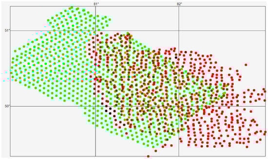
Figure 1. Spatial distribution of geochemical sampling points (red) and generated grid points (green) used for constructing prediction maps within the study area. Color intensity variations reflect differences in gold concentration for sampling points.

In the northwestern direction, a total of 820 prediction points were generated (Figure 1, green points). A portion of these generated points is located within an area covered by a thick layer of unconsolidated deposits, where geochemical sampling data are absent (i.e., no red points are present). All generated points are displayed with identical color intensity, as the gold content at these locations is unknown.

The objective of this study is to forecast the gold concentration at the generated points using information from locations with available geochemical analysis results. For this purpose, a multilayer perceptron model is trained on the dataset presented in Table 1 and subsequently applied to predict gold content at unsampled locations.

We consider the problem statement in more detail. There is a set of sampling points with coordinates ($X_i$, $Y_i$), and at each sampling point the gold content $C_i$ is known. We will use a multilayer perceptron (MLP) as a function or operator that maps the coordinates of a sampling point ($X_i$, $Y_i$) to the content of the element under study $C_i$:

MLP: (X,Y)⟶C

(1)

The data from Table 1 will be used as the training dataset. In this case, the number of input neurons in the MLP will be equal to 2, corresponding to the two coordinates (X,Y), and the number of output neurons will be one, corresponding to the value of C at point (X,Y). Now, to fully define the MLP architecture, it is necessary to determine the number of hidden layers and the number of neurons in each hidden layer.

With respect to the selection of the number of hidden layers, this study follows the results of a fundamental work in the theory of feed-forward neural networks, including multilayer perceptrons, devoted to the universal approximation property [11]. The results presented in [11] address the problem of function representability within the class of neural networks with a single hidden layer and demonstrate that arbitrary continuous functions defined on compact domains can be approximated with arbitrary accuracy by feed-forward neural networks containing only one hidden layer and employing a continuous sigmoidal activation function. Consequently, an MLP with a single hidden layer and a sigmoidal nonlinearity is theoretically capable of approximating functions of arbitrary complexity, including those arising in problems of type (1).

The number of neurons in the hidden layer is selected experimentally based on the results of numerical experiments and model performance evaluation.

To implement the multilayer perceptron, custom software developed in the C# programming language was used. The software has been validated on several benchmark problems, including a classification task involving handwritten digit recognition using the MNIST dataset [12], demonstrating the correctness and stability of the implemented neural network framework.

2. Materials and Methods

In the present study, a multilayer perceptron (MLP) is selected as the predictive model. Owing to its universal approximation capability, the MLP is able to represent complex nonlinear relationships without requiring an explicit specification of the underlying functional form. This property makes it particularly suitable for the analysis of spatial patterns in geochemical data, especially in cases where prior knowledge of the relationships between variables is limited. At the same time, it is well recognized that the predictive performance of neural network models strongly depends on both the quality of the input data and the structure of the feature space.

Accordingly, the application of the MLP in this work is combined with a preliminary preprocessing of the input spatial coordinates aimed at increasing feature informativeness and partially compensating for the weak spatial correlations inherent in the original dataset. This preprocessing step is intended to improve the learning efficiency and predictive stability of the neural network model.

2.1. Baseline MLP Architecture and Numerical Experiment Setup

The computational experiments consisted of the following stages:

(1) Normalization of input data: this is the process of mapping the domain of the input data to the interval [0, 1] or [−1, 1]; for each input neuron, the minimum and maximum values across all training data are determined, after which the input data are normalized to the interval [0, 1] or [−1, 1]. In our case, all input data were normalized to the interval [0, 1] using the following formulas:

for the interval [0, 1];

for the interval [−1, 1];

(2) Random (randomized) selection of weight and bias values: based on empirical experience with network weight and bias randomization, it is recommended to alternate the selection of each weight and bias within the intervals [−1, 0] and [0, 1];

(3) Selection of the learning rate: this is a parameter used to limit the magnitude of the weight adjustment at each update, which affects the speed of minimizing the objective function; in our case, this coefficient was set to 0.2;

(4) The number of training epochs of the objective function, which is selected experimentally and depends on the rate at which the objective function converges to 0;

(5) Definition of the type of objective function: in the experiment, two types of objective functions were calculated:

$$\begin{array}{c}{F}_{1 }\left(w,b\right)={\displaystyle \frac{1}{N}}{\displaystyle \sum _{i=1}^N}{\left(f_i^{*}-f_i\right)}^2\\ F_{2 }\left(w,b\right)={\displaystyle \frac{1}{N}}{\displaystyle \sum _{i=1}^N}\left(f_i^{*}-f_i\right)\end{array}$$

(2)

The first objective function is defined as the arithmetic mean of the squared residuals between the true values of the target variable and the values predicted by the network, computed over the entire training dataset within a single training epoch. The second objective function is defined as the mean absolute residual between the true target values and the corresponding network predictions, evaluated over the full training dataset within the same epoch.

(6) Direct execution of a series of tests.

The main parameters of the numerical experiments are as follows:

−

Input neurons: 2—longitude and latitude coordinates;

−

Output neurons: 1—Au content at the sampling point;

−

Number of hidden layers: 1;

−

Initial number of neurons in the hidden layer: 150;

−

Number of epochs: 200.

2.2. Feature Transformation Methodology Based on Anisotropy Modeling and Dual-MLP Training

Feature transformation methodology based on constructing an informational and mathematical anisotropy model for the prediction points, and preparation of the training dataset and prediction set for computation using a multilayer perceptron. As is known, anisotropy in geological information manifests itself as the dependence of medium properties on direction. In geology, anisotropy is understood as the dependence of the variability of geological indicators on spatial directions. For example, the variability anisotropy of the contents of different ore components within an ore body is often non-uniform, which is a consequence of the specific stages of its formation. Physically, anisotropy may be associated with fine layering, elongated shapes of soil particles, fracturing, ice content, metamorphism, and the stress–strain state—that is, with lithological, structural, textural, and tectonic properties of rocks, as well as other causes [13,14].

In the present study, the focus is placed on the anisotropy of mineral content, understood as the directional variability of mineral concentrations with respect to the prediction direction. The geological sampling data are summarized in Table 1, while their spatial distribution is illustrated in Figure 1, which shows the locations of the geochemical sampling points. The color intensity of the points reflects the corresponding concentration values, with darker shades indicating higher mineral content. Points displayed with uniform color denote locations for which geochemical assay results are unavailable.

The prediction task is formulated as follows: for the generated points located in the northwestern direction, the gold concentration (Au1) must be forecasted. Accordingly, the analysis is focused on the directional variability of mineral content specifically along the northwest direction.

Convex hulls are constructed for the set of geochemical sampling points and for the set of generated points [15]. Figure 2 illustrates the convex hulls used to visually represent the spatial boundaries of the original data and the area within which the predicted values are generated.

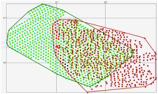
Figure 2. Spatial distribution of geochemical sampling points (red) and generated computational grid nodes (green), together with their corresponding convex hulls, which define the boundaries of the area used for modeling and constructing prediction maps. Color intensity variations reflect differences in gold concentration for sampling points.

We introduce the following notation: R is the set of points with geochemical sampling results (red), and G is the set of generated points (green), then: C is the union of these sets: C = R∪G, S—the intersection of these sets: S = R∩G, R_G—the difference in the sets: R_G = R\G, G_R—the difference in the sets: G_R = G\R. Then, based on the adopted notation: G_R—the set of generated points located in the area covered by a thick layer of unconsolidated deposits; S_R—the set of generated points belonging to the intersection of the sets S = R∩G; S_G—the set of points with known geochemical analysis results belonging to the intersection of the sets S = R∩G.

Thus, the problem of forecasting gold content at the points of set G is divided into the following two tasks:

To forecast the gold content at the points of set S_R—essentially an interpolation problem, i.e., estimating the unknown gold content values at the points of set S_R, which are located between the points of set S_G with known geochemical analysis results.

To forecast the gold content at the points of set G_R—essentially an extrapolation problem, i.e., estimating the unknown gold content values at the points of set G_R, which are located outside the set of points S_G with known geochemical analysis results.

The methodology for solving the interpolation problem for the unknown gold content values at the points of set S_R.

Given that in this case we are interested in the variation of gold content in the northwest direction, determine the equations of the straight lines along which the mineral content will be forecasted for the points of sets R and G. To do this, we place both sets on a single figure, determine the correlation lines for these sets, and display them in Figure 3. As can be seen, the correlation lines of these sets are almost parallel.

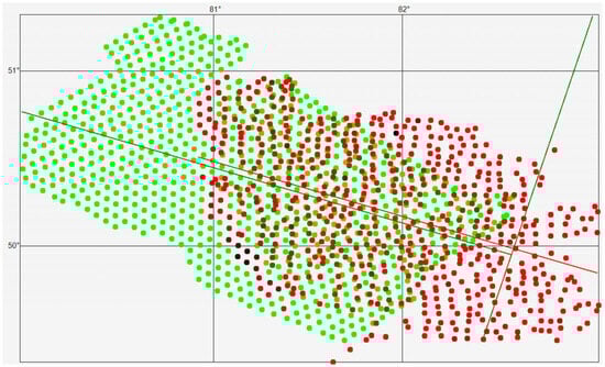
Figure 3. Geological sampling points and generated points used for prediction, together with correlation lines highlighting the weak direct relationship between spatial coordinates and geochemical values.

We will consider the anisotropy of the mineral content along the correlation lines in the northwest direction, as shown in Figure 3.

The concept of “anisotropy converging to a point” is introduced. For the geometric interpretation of this concept, we define the following objects and introduce several terms. We define the prediction line as the straight line perpendicular to the correlation line—shown in Figure 3 as the green line perpendicular to the correlation line of set G. Essentially, the prediction line drawn through a prediction point divides the plane into two half-planes: the southeast half-plane (the right half-plane), which must always contain points with known geochemical sampling results, and the northwest half-plane (the left half-plane), which contains the prediction points, i.e., points without geochemical sampling results.

In particular, in Figure 3, southeast of the prediction line (the green line perpendicular to the correlation line of the generated set) are the red points for which geochemical sampling results are known, while northwest of the prediction line are the green points for which the mineral content must be forecasted. Note that points with known geochemical sampling results may also lie in the left half-plane. Thus, for forecasting, it is necessary to select such a point from the prediction set R that, when the prediction line is drawn through it, there is a certain number of geochemical sampling points located to the right of this line.

The rules for selecting the point for which the anisotropy model must be constructed and/or the mineral content must be forecasted (hereinafter referred to as the prediction point) as follows: we choose such a prediction point p from the prediction set that, if the prediction line is drawn through it, there must be a subset of geochemical sampling points located to the right of this prediction line, and the points of this subset closest to the prediction line must lie no farther from it than the maximum distance between neighboring points of set G.

Let there be a prediction point p, through which the prediction line AB passes (Figure 3). We divide the right half-plane into S_i sectors (i > 1), and each sector is further divided into subsectors P_ij, where a subsector is defined as the part of a sector bounded by two arcs of different radii r_j (j > 1); moreover, the first sector is bounded on the angular side by the prediction point p itself.

In Figure 4, p is the prediction point; AB is the prediction line; the right half-plane AB^Π is divided into three sectors: S₁ = ApD, S₂ = DpC, S₃ = CpB; each sector is in turn divided into three subsectors according to the radii r₁, r₂, r₃.The number of divisions is chosen for demonstration purposes—in principle, the division may be made into any reasonable number of sectors and subsectors.

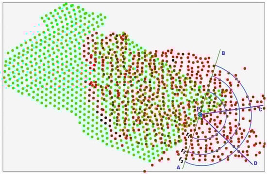
Figure 4. Geometric construction illustrating the information measure based on the subdivision of the half-plane into angular sectors and radial subsectors used for analyzing the spatial distribution of geochemical sampling points.

The following conditions are imposed on the sector subdivision. Let N be the total number of points in the right half-plane for which geochemical sampling results are known, and let N_S be the number of sectors into which the right half-plane AB^Π must be divided. Then the sectors should be constructed such that each sector contains N/N_S points with known geochemical sampling results. For definiteness, the integer remainder of the division N/N_S is added to the last sector. For example, if N = 100, N_S = 3, the remainder is 1, and therefore the first sector should contain 33 points, the second sector 33 points, and the third sector 34 points.

Now consider the subdivision of sectors into subsectors using sector S₁ as an example. In this sector, the first subsector P₁₁ is bounded on one side by point p and on the other by the arc of radius r₁; the second subsector P₁₂ is the part of sector S₁ bounded by the arcs of radii r₁ and r₂; the third subsector P₁₃ is the part of sector S₁ bounded by the arcs of radii r₂ and r₃. In principle, a fourth subsector may also be introduced, bounded on one side by radius r₃ and practically unbounded within the sector on the other, but in this case, we restrict ourselves to only three subsectors.

In the presented example, the right half-plane is divided into three angular sectors, and each sector is further subdivided into three radial subsectors. As noted earlier, both the number of sectors in the half-plane and the number of subsector divisions can be selected arbitrarily. The choice of these parameters depends on the type of mineral under investigation, the spatial distribution and density of sampling points, and other geological and methodological considerations.

Figure 4 illustrates the geometric construction used to define the proposed information measure. In this example, the right half-plane is partitioned into three angular sectors, each of which is further subdivided into three radial subsectors, forming a structured directional representation of the spatial neighborhood. The number of sectors and subsectors can be selected depending on the mineral type, the spatial distribution of sampling points, and other relevant factors. After completing the required geometric constructions, we proceed to analyze the points with known geochemical assay results that fall within each subsector. Let us denote by M_ij the set of points located in subsector P_ij of sector S_i, where

i ∈ [1, …, N_S], j ∈ [1, …, N_P] and where N_S is the number of sectors into which the right half-plane is divided, and N_P is the number of subsectors within each sector.

We then compute the average concentration of the mineral C_ij for subsector P_ij using the following formula:

$$C_{ij}={\displaystyle \frac{{\displaystyle \sum _{k=1}^{\left|M_{ij}\right|}{c}_{ij}^k}}{\left|M_{ij}\right|}}$$

(3)

where C_ij is the average concentration of the mineral within subsector P_ij; $c_{ij}^k$ denotes the geochemical assay result (mineral content) at the k-th point located in subsector P_ij; and |M_ij| is the cardinality of the set M_ij i.e., the number of points contained in that subsector.

We now compute the coordinates corresponding to the considered subsector using the following formulas:

$$Lo{n}_{ij}={\displaystyle \frac{{\displaystyle \sum _{k=1}^{\left|M_{ij}\right|}lo{n}_{ij}^k}}{\left|M_{ij}\right|}}$$

(4)

where

$Lo{n}_{ij}$—the weighted average geographic longitude of all points in the set M_ij;

$La{t}_{ij}$—the weighted average geographic latitude of all points in the set M_ij;

$lo{n}_{ij}^k$—the geographic longitude of the k-th point in the set M_ij;

$la{t}_{ij}^k$—the geographic latitude of the kk-th point in the set M_ij;

and |M_ij|—the cardinality of the set M_ij, i.e., the number of points in that subset.

We now construct an information model of anisotropy converging to the point p. Here, an information model is understood as a model of an object—in this case, a model of anisotropy converging to the point p—represented in the form of information that describes the parameters and variable quantities of the object which are essential for the study and are mutually related.

The essential constituent elements of the information model of anisotropy converging to the prediction point p_i are:

The prediction point, which is described by

−

its geographic coordinates: longitude loniloni and latitude latilati;

−

the concentration c_i of the mineral at the point p_i∈R.

The average concentration $C_{lm}^i$ of the mineral for subsector $P_{lm}^i$, where

l is the number of the sector in the information model of anisotropy converging to the point p_i, and m is the number of the subsector of sector l corresponding to the prediction point p_i ∈ R;

The weighted average geographic coordinates—$Lo{n}_{lm}^i$ and $La{t}_{lm}^i$—are for the subsector $P_{lm}^i$ i of the prediction point p_i ∈ R.

As an example, we present in tabular form the information model of anisotropy converging to the point pp (Figure 4) for the first sector:

An information model describing the parameters and variables involved in anisotropy analysis is presented in Table 2.

Table 2. Information model of anisotropy converging to point p for a single sector.

№	Element of the Information Model	Designation	Description
1	Geographic longitude	lon	Geographic longitude of point p
2	Geographic latitude	lat	Geographic latitude of point p
3	Mineral content at point p	c	Mineral content at point p
4	Average mineral content in subsector 1 of sector 1	C11	Mineral content in the subsector
5	Weighted average longitude of subsector 1 of sector 1	Lon11	Geographic longitude
6	Weighted average latitude of subsector 1 of sector 1	Lat11	Geographic latitude
7	Average mineral content in subsector 2 of sector 1	C12	Mineral content in the subsector
8	Weighted average longitude of subsector 2 of sector 1	Lon12	Geographic longitude
9	Weighted average latitude of subsector 2 of sector 1	Lat12	Geographic latitude
10	Average mineral content in subsector 3 of sector 1	C13	Mineral content in the subsector
11	Weighted average longitude of subsector 3 of sector 1	Lon13	Geographic longitude
12	Weighted average latitude of subsector 3 of sector 1	Lat13	Geographic latitude

As noted above, an information model describes the parameters and variable quantities of the object under study that are essential and mutually interrelated. Traditionally, anisotropy in geochemical data is characterized using assay values at sampling points through the identification of principal directions of spatial correlation or by means of spatial variogram models [16,17].

In the present study, however, anisotropy is represented using an alternative information model formulated as an ordered sequence of variations in the averaged mineral concentration values and the weighted average coordinates of subsectors within the defined sectors. These quantities are computed according to Formulas (3) and (4) as the subsectors converge toward the prediction point, thereby providing a directional and structured representation of spatial variability.

Based on this ordered sequence of averaged mineral concentration values in the subsectors as they converge toward the prediction point p, it becomes possible to construct, for each i-th sector, a functional relationship of the following general form:

$$Content=f_i(r)$$

(5)

Content—the mineral concentration in the considered sector as a function of the radius length r, with $r\in \left[0,r_{Np}\right]$, $N_P$ is the number of subsectors in the considered sector;

$i\in \left[1,\dots ,N_S\right]$, where $N_S$ is the number of sectors for the p-th prediction point;

–f_i(r)—the function describing the variation in mineral concentration for the i-th sector, which must be constructed from the data in the following table containing the mineral concentration values and their corresponding radii:

The radius values r_i in Table 3 are computed using the following formulas:

$$r_i=\sqrt{{(Lo{n}_{ij}-lon)}^2-{(La{t}_{ij}-lat)}^2}$$

(6)

Table 3. Initial data for constructing dependence (5) for the i-th sector. Dots indicate omitted intermediate rows; NpN_pNp denotes the total number of points in the sector.

№	Mineral Content	Radius
1	c	0
2	Ci1	r1
3	Ci2	r2
…	…	…
Np	CiNp	rNp

There exist numerous methods for approximating tabulated data by various types of functions [18], which is used to construct a functional dependence of the mineral content on the radius length. Furthermore, all sectors of the prediction point p must be approximated by functions of the same type, and, in addition, all functions describing the relationships in (6) must satisfy the following condition at r = 0:

$$f_1(0)=f_2(0)=\dots =f_{Ns}(0)=c$$

(7)

which means that, for any sector $i\in \left[1,\dots ,N_S\right]$, the value of function (5) at the point r = 0 must be equal to the numerical value of the mineral content c at point p.

Thus, all prediction points of the considered sets must satisfy Equations (5) and (7).

Next, the number of functions N_f of type (5) that must be approximated based on Tables of type 3 for the prediction set P:

N_f = N_S × |P|

(8)

where N_S is the number of sectors used to construct the anisotropy model converging to the point;

|P| is the cardinality of the set P.

For example, for the set P shown in Figure 1, the cardinality is |P| = 820.

If we construct N_S = 3 sectors for each prediction point, then we must build 820 × 3 = 2,460,820 × 3 = 2460 functions approximating 2460 tables of type 3.

As noted earlier, such a task can most effectively be addressed today using multilayer perceptrons. Therefore, instead of constructing functions of type (5), we shall approximate the anisotropy of mineral concentration values converging to the point—represented in the form of a Table of type 3—using MLP.

The information model of anisotropy converging to a point is then transformed into a form suitable for input into a neural network. We represent the data from Table 3 as a single row of a training set corresponding to one sector of the selected prediction point pp.

Such a row, when forming the training dataset, will have the structure shown in Table 4 below:

Table 4. Format of a single training-set row representing the information for one sector.

lon	lat	C11	C12	C13	Lon11	Lat11	Lon12	Lat12	Lon13	Lat13	c
1	2	3	4	5	6	7	8	9	10	11	12
81.801	49.477	0.247	0.169	0.417	81.904	49.492	82.109	49.550	82.279	49.600	0.114

Table 4 is constructed for the case in which each prediction point is represented by N_S = 3 sectors, and each sector is divided into N_P = 3 subsectors. Under these conditions, the first 11 parameters in Table 4 serve as input data for the MLP, while the 12-th parameter represents the output training target of the MLP, which in this case corresponds to the mineral content at the prediction point. During MLP training, the output neuron value for a given set of input parameters must converge to the value specified by the 12-th parameter.

Each row must be stored in CSV format (Comma-Separated Values)—a standard text format for tabular data representation.

Given the specifics of training and solving prediction problems using MLP, the prediction points p fall into two categories:

−

Prediction points used for training the neural network, i.e., points for which the mineral content is known;

−

Actual prediction points, i.e., points at which the mineral content must be determined.

In the general case, for a prediction point pp, whose right half-plane is divided into N_S sectors and each sector into N_P subsectors, a single row of input parameters in the training dataset corresponding to one sector will contain (3 × N_P + 2) input parameters and one output parameter—the mineral content at point pp.

Therefore, the total number of rows corresponding to prediction point pp will be equal to N_S.

When forming the MLP training set for N prediction points, the total number of rows in the prediction dataset will be: N × N_S. Moreover, for all N_S rows corresponding to a particular prediction point pipi, the value of the output parameter will be identical.

An MLP trained on such data will produce, for each prediction point, N_S predicted mineral content values corresponding to its sectors. To obtain the final predicted value of mineral concentration at the prediction point, we refer to condition (7). According to this condition, all values of function (5) at r = 0 must be equal to one another. Therefore, to ensure that the MLP output values for each sector satisfy condition (7), we apply a second multilayer perceptron as follows.

From the N_S predicted mineral content values obtained for each sector of the prediction point, we construct a row of the training dataset whose format is presented in the following table:

For validation of the MLP model, the performance metrics defined in Equation (2) were used:

−

The first objective function (MSE), defined as the mean squared error between the desired value of the target variable and the value computed by the network over the entire training dataset within a single training epoch;

−

The second objective function (MAE), defined as the mean absolute error between the desired value of the target variable and the value computed by the network over the entire training dataset within a single training epoch.

The data presented in Table 1 were used to form the training and testing datasets. The dataset was divided into two subsets in a 50%/50% proportion, where samples with even indices were assigned to the training set and samples with odd indices were assigned to the test set.

Table 5 presents the results of training the MLP model using the data from Table 4.

Table 5. Results of MLP training on the training dataset.

Epoch	MSE	MAE
0	0.82077474500391	0.893272247249522
1	0.820599694291198	0.893175360864609
2	0.818636895067488	0.892059802696424
3	0.0502519954187467	0.117690478980947
4	0.0194282358030462	0.0810368016925656
…	…	…
318	0.00999956637843734	0.062808014924875
319	0.00999822905717217	0.0628035038892045
…	…	…
498	0.00982753810774244	0.0622917764594883
499	0.0098268880956763	0.0622898131791592

After training, the MLP model was evaluated on the test dataset. The testing results demonstrated that the test error did not exceed an MSE value of 0.015.

In columns 1, 2, and 3, the values of mineral concentration computed by the trained multilayer perceptron, based on the data given in Table 4 for a single prediction point, are presented, while the fourth column contains the true value.

To satisfy condition (7), we form for each prediction point one row in the format shown in Table 6. These rows together constitute the training dataset for a second multilayer perceptron, which must have the following basic parameters:

−

Number of input neurons: 3 (equal to the number of sectors N_S);

−

Number of output neurons: 1.

After training the multilayer perceptron on this dataset, we obtain, for each prediction point, the final neural-network-predicted value of mineral concentration at point p.

If we pass the prediction-set points, prepared using the information model of anisotropy converging to the point, through the trained neural network, the network will compute the predicted mineral concentration values.

Thus, to predict mineral concentration values based on the information model of anisotropy of mineral content converging to the point—described by Equations (5) and (7)—we employ a multilayer perceptron twice.

Table 6. Format of a single training-set row used to obtain a single predicted concentration value at the prediction point.

C1	C2	C3	c
1	2	3	4
0.3251	0.2653	0.3201	0.2894

Table 6. Format of a single training-set row used to obtain a single predicted concentration value at the prediction point.

C1	C2	C3	c
1	2	3	4
0.3251	0.2653	0.3201	0.2894

Algorithm for Solving the Prediction Problem Using Preliminary Processing of Geological Input Data and Dual Application of a Multilayer Perceptron

The methodology for solving the interpolation problem of unknown gold concentrations at the points of set S_R can be presented in the form of the following algorithm:

1. Consider the sets:

S_R—the set of generated points belonging to the intersection of the sets S = R∩G;

S_G—the set of points with known geochemical assay results belonging to the intersection S = R∩G;

The information about the points of set S_G forms the training sample.

2. Specify the values: N_S, N_P, r₁, r₂, …, r_NP.

3. For every p∈S_G, compute using Formulas (3) and (4) the average concentration and the weighted average coordinates for each subsector.

4. For every p∈S_G, construct the information model of anisotropy converging to point pp.

The information for each sector is presented as a single row of the training set.

For each prediction point p, N_S rows must be formed in CSV format.

5. Define the architecture of the multilayer perceptron (the first neural network):

−

Specify the number of input neurons (3 × N_P + 2);

−

Specify the number of output neurons: 1;

−

Specify the number of hidden layers;

−

Specify the number of neurons in the hidden layer(s);

−

Specify the normalization regime for the input data—each input variable is normalized individually.

6. Specify the number of training epochs.

7. Run the neural network for training.

8. Obtain and process the results.

9. From the outputs corresponding to all N_S rows produced by the first neural network, and in accordance with the structure shown in Table 6, construct |S_G| rows of the training dataset for the second perceptron, where |S_G| is the cardinality of the set S_G.

10. Define the architecture of the second multilayer perceptron (the second neural network):

−

Number of input neurons: 3;

−

Number of output neurons: 1;

−

Number of hidden layers;

−

Number of neurons in the hidden layer(s);

−

Specify the normalization regime for the input data—each input variable is normalized individually.

11. Specify the number of training epochs.

12. Run the neural network for training.

13. Obtain and process the results.

14. We now proceed to solving the interpolation problem, i.e., determining the gold concentration at the points of the set S_R. In this case, the prediction set will be prepared based on the set R.

15. Specify the values: N_S, N_P, r₁, r₂, …, r_NP.

16. For every p∈S_R, compute, using Formulas (3) and (4), the average concentration and the weighted average coordinates for each subsector.

17. For every p∈S_R construct the information model of anisotropy converging to point p. The information for each sector is represented as a single row of the training set. Thus, for each point pp, N_S rows must be generated in CSV format.

18. Run the first neural network to perform prediction.

19. Obtain and process the results.

20. From the values of all N_S output neurons, and in accordance with the structure shown in Table 6, form |S_R| rows of the training dataset for the second neural network.

21. Run the second neural network to perform prediction.

22. Obtain and process the results.

3. Results

3.1. Evaluation of the Baseline MLP Model

Based on the calculation results, a plot of the variation in objective function (2) as a function of the number of completed epochs—the mean absolute residual between the desired value of the target variable and the value of the target variable computed by the network over the entire training set within a single epoch—was constructed, as shown in Figure 5.

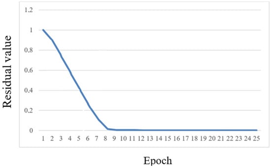
Figure 5. Evolution of the objective (loss) function as a function of training epochs for the MLP model with 150 hidden neurons, demonstrating the convergence and stability of the learning process.

As can be seen from Figure 5, the value of the objective function decreases sharply after 8 epochs of computation and converges almost to zero.

We determine the range of Au1 values in the training dataset and the range of Au1 values computed by the neural network, and then compare them.

Let O denote the set of Au1 content values used as the training dataset:

$$O=\left\{Au1\in \left[0.1052÷4.95\right]\right\}$$

(9)

Let C denote the set of Au1 content values computed by the neural network:

$$C=\left\{Au1\in \left[0.105276÷0.117664\right]\right\}$$

(10)

As can be seen from (9) and (10), the range of values in the training dataset is significantly wider than the range of values computed by the neural network—by more than a factor of 240. At the same time, the statistical characteristics of the two sets are as follows: for set O − M(XO) = 0.349931, D(XO) = 0.09578, for set C − M(XC) = 0.107590, D(XC) = 6.6215 × 10⁻⁶. he correlation coefficient between the training dataset and the computed values is −0.06341−0.06341 −0.06341.

Increasing the number of neurons in the hidden layer resulted in even worse outcomes, i.e., the range of the computed Au1 values became even narrower and the variance D(XC) decreased significantly, while the behavior of the objective function remained consistent with that shown in Figure 5.

Therefore, the number of neurons in the hidden layer was reduced, and the range of the computed Au1 values began to increase, reaching its maximum when there was only one neuron in the hidden layer:

−

Input neurons: 2—longitude and latitude coordinates;

−

Output neurons: 1—Au1 content at the sampling point;

−

Hidden layers: 1;

−

Number of neurons in the hidden layer: 1.

For this neural network, the following data were obtained for the computed set of Au1 content values:

$$C=\left\{Au1\in \left[0.113856÷0.297424\right]\right\}$$

(11)

In this case, for the computed Au1 values: M(XC) = 0.126167, D(XC) = 0.000262, and the correlation coefficient between the training set and the set of computed values is −0.02572.

For the considered calculation variant, the plot of the mean absolute residual between the desired value of the target variable and the value of the target variable computed by the network over the entire training set as a function of the epoch number is shown in Figure 6.

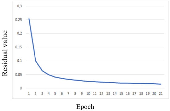
Figure 6. Variation in the objective (loss) function with the number of training epochs for the MLP configuration with a single neuron in the hidden layer.

As can be seen, even the wider range (11) is still more than 26 times narrower than the range of the input data, i.e., the neural network was unable to establish a stable correlation relationship between the training dataset and the computed Au1 values, which is confirmed by the very low correlation coefficient between the training dataset and the computed Au1 values.

Nevertheless, construct a forecast of the Au1 content for the generated points in the northwest of the study area for the considered MLP, which is visually presented in Figure 7.

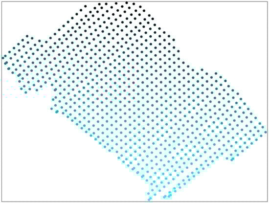
Figure 7. Predicted Au1 concentration values at generated points in the northwestern part of the study area produced by an MLP model with one hidden neuron, applied without prior data preprocessing.

As can be seen from Figure 7, the multilayer perceptron produces an overly simplified spatial pattern, characterized by a monotonic increase in gold concentration from east to west. Although this general trend is present in the data, the actual spatial distribution of gold content is considerably more complex, as illustrated in Figure 1, where the red points of varying color intensity represent the measured concentrations at geochemical sampling locations. Notably, for the generated points located in the vicinity of the training samples, the range of predicted gold concentrations is even narrower than that obtained using expression (11).

This result highlights a fundamental limitation of the direct modeling approach: the relationship between the spatial coordinates of sampling points and the corresponding geochemical assay values is weak, indicating a low level of correlation between the input variables and the target variable. Consequently, direct application of the multilayer perceptron fails to capture the underlying spatial variability of the geochemical field. To address this issue, preprocessing of the training dataset is required in order to enhance the dependency between the input and output variables through appropriate feature transformation techniques [19,20].

3.2. Prediction Results with Anisotropy-Based Preprocessing and Dual MLP

After applying the anisotropy-based feature transformation and the dual-stage MLP procedure described in Section 2.2, the final predicted gold concentrations were obtained for all points of the generated set S_R. These predicted values represent the output of the second MLP, which aggregates sector-based estimates into a single final concentration value for each prediction point.

Omitting the details of the computational procedures described in Section Algorithm for Solving the Prediction Problem Using Preliminary Processing of Geological Input Data and Dual Application of a Multilayer Perceptron (which constitute the subject of a separate article), we note that the final result consists of the predicted gold concentration values at the points of the set SR, presented in Figure 8.

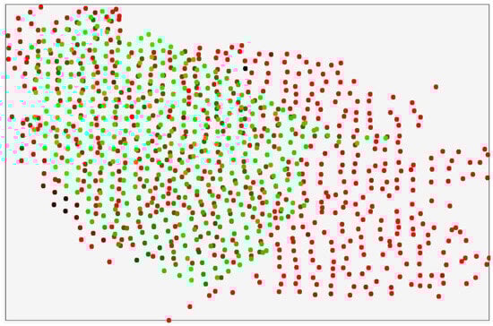
Figure 8. Spatial distribution of the set S_R of generated points (green), where gold concentration values are predicted, and the set R of geochemical sampling points (red) with known assay results, illustrating the separation between observed data and prediction locations.

The training process of the MLP model demonstrates a stable and monotonic decrease in both MSE and MAE values over successive epochs (Table 5). A rapid reduction in the error is observed during the initial training stage, followed by gradual convergence, indicating effective learning and numerical stability of the network.

After approximately 300 epochs, the training error reaches a plateau, with final values of MSE ≈ 0.0098 and MAE ≈ 0.062, suggesting convergence of the optimization process. The testing phase further confirms the robustness of the trained model. The MSE computed on the independent test dataset does not exceed 0.015, which is comparable to the training error level.

The absence of a significant discrepancy between training and testing errors indicates that the model does not suffer from pronounced overfitting and retains its predictive capability for unseen data within the surveyed area. While prediction maps provide a qualitative representation of spatial distribution patterns, the reported quantitative error metrics offer an objective assessment of the predictive performance of the MLP model.

4. Conclusions

A major challenge in training MLP for solving prediction problems on datasets of the type presented in Table 1 is that such models tend to produce significantly simplified prediction results.

The simplified nature of the prediction results from the low informativeness of the original input data and the weak correlation between the input variables and the target variable (i.e., the output neuron) in the training set. To enhance the dependency between the input and output variables, it is therefore necessary to perform preliminary preprocessing of the training dataset using appropriate feature transformation techniques.

The introduction of the concept of anisotropy converging to a point enables the construction of training datasets with significantly increased correlation between the transformed input features and the predicted output values. This, in turn, motivates the dual application of a multilayer perceptron within the prediction workflow, allowing the model to more effectively capture directional spatial variability in the geochemical field.

Quantitative validation using the MSE and MAE metrics demonstrated stable convergence of the training process and consistent model performance on independent test data, indicating the reliability of the proposed approach within the surveyed area.

Future research will focus on extending the proposed methodology to other geochemical elements and regions, as well as on investigating model behavior under strict extrapolation conditions and incorporating additional validation strategies.

References

- Los, V.L.; Legonkin, V.S. development of mathematical and software tools For forecasting ore deposits. Elan software package. Geol. Subsoil Prot. 2025, 3, 50–64. [Google Scholar]
- Pei, J.; Zhang, Y. Prediction of reservoir fracture parameters based on the multilayer perceptron machine-learning method: A case study of Ordovician and Cambrian carbonate rocks in the Nanpu Sag, Bohai Bay Basin, China. Processes 2022, 10, 2445. [Google Scholar] [CrossRef]
- Ji, Y.; Kim, H.-S.; Lee, M.-G.; Cho, H.-I.; Sang, C.-G. 3D mapping of geotechnical layers based on MLP using a borehole database in Seoul, South Korea. J. Korean Geotech. Soc. 2021, 37, 47–63. [Google Scholar] [CrossRef]
- Tsae, N.B.; Adachi, T.; Kawamura, Y. Application of artificial neural network for the prediction of copper ore grade. Minerals 2023, 13, 658. [Google Scholar] [CrossRef]
- Sánchez Rodríguez, S.; Sampedro, G.; Fernández, J.D.; López, J.D. Predicting rock mass conditions ahead of tunnel face and the use of geostatistical methods. A comparative study. In Proceedings of the ISRM International Symposium—EUROCK 2020, Trondheim, Norway, 14–19 June 2020; p. ISRM-EUROCK-2020-152. Available online: https://onepetro.org/ISRMEUROCK/proceedings-abstract/EUROCK20/All-EUROCK20/447397 (accessed on 15 June 2021).
- Yasrebi, A.B.; Hezarkhani, A.; Afzal, P.; Karami, R.; Eskandarnejad Tehrani, M.; Borumandnia, A. Application of an ordinary kriging–artificial neural network for elemental distribution in Kahang porphyry deposit, Central Iran. Arab. J. Geosci. 2020, 13, 748. [Google Scholar] [CrossRef]
- Kaplan, U.E.; Topal, E. A new ore grade estimation using combine machine learning algorithms. Minerals 2020, 10, 847. [Google Scholar] [CrossRef]
- Hou, X.-Z.; Yang, Z.-F.; Wang, Z.-J. The occurrence characteristics and recovery potential of middle–heavy rare earth elements in the Bayan Obo deposit, Northern China. Ore Geol. Rev. 2020, 126, 103737. [Google Scholar] [CrossRef]
- Yeh, I.-C.; Huang, K.-C.; Kuo, Y.-H. Spatial interpolation using MLP–RBFN hybrid networks. Comput. Geosci. 2007, 33, 102–113. [Google Scholar]
- Akhmetov, D.S.; Los, V.L. Solving the problem of ore grade prediction using artificial neural networks. Geol. Subsoil Prot. Kazakhstan 2023, 1, 58–62. [Google Scholar]
- Cybenko, G. Approximation by superpositions of a sigmoidal function. Math. Control Signals Syst. 1989, 2, 303–314. [Google Scholar] [CrossRef]
- LeCun, Y.; Cortes, C.; Burges, C.J.C. MNIST Handwritten Digit Database. 2025. Available online: http://yann.lecun.com/exdb/mnist/ (accessed on 15 September 2025).
- Erofeeva, G.V.; Erofeev, L.Y. On the methodology of assessing and geologically interpreting anisotropy of physical fields. Izv. Tomsk Polytech. Univ. 2012, 320, 87–91. [Google Scholar]
- Shevnin, V.A.; Karinsky, A.D.; Yalov, T.V. Study of Azimuthal Resistivity Anisotropy Using Dipole–Dipole Electromagnetic Profiling. In Proceedings of the EAGE Near Surface Conference, Paris, France, 3–5 September 2012. [Google Scholar]
- Algorithmica. Convex Hulls. Available online: https://algorithmica.org/ru/convex-hulls (accessed on 14 November 2025).
- Redkin, G.M.; Gerasimov, A.V.; Aleksanov, V.Y. Anisotropy of geological indicator variability. Min. Inf. Anal. Bull. 2012, 165–168. Available online: https://drive.google.com/file/d/14Kx1LblOHfGdQmgrynGqUExm4a2qrvSL/view?usp=sharing (accessed on 22 September 2025).
- Skrubite, R.A.; Fakhrutdinov, S.I. Geological basis for detecting anisotropic directions in geostatistical modeling: A case study of the Verkhnee ore body of the Mnogovershinnoye gold deposit. Proc. High. Educ. Inst. Geol. Explor. 2022, 64, 73–85. [Google Scholar]
- Malysheva, T.A. Numerical Methods and Computer Modeling. Laboratory Practicum on Function Approximation; ITMO University: Saint Petersburg, Russia, 2016; p. 33. Available online: https://drive.google.com/file/d/1MDKqeiCWMehcINq_–hdKZ5w9gsdZLElf/view?usp=sharing (accessed on 15 June 2022).
- Zhuang, H.; Wang, X.; Bendersky, M.; Najork, M. Feature Transformation for Neural Ranking Models. In Proceedings of the 43rd International ACM SIGIR Conference on Research and Development in Information Retrieval, Virtual Event, China, 25–30 July 2020; pp. 1649–1652. [Google Scholar]
- Heaton, J. Automated Feature Engineering for Deep Neural Networks with Genetic Programming; College of Engineering and Computing, Nova Southeastern University: Davie, FL, USA, 2016; p. 53. Available online: https://www.heatonresearch.com/dload/phd/jheaton–nsu–phd-idea-paper.pdf (accessed on 15 June 2024).
Disclaimer/Publisher’s Note: The statements, opinions and data contained in all publications are solely those of the individual author(s) and contributor(s) and not of MDPI and/or the editor(s). MDPI and/or the editor(s) disclaim responsibility for any injury to people or property resulting from any ideas, methods, instructions or products referred to in the content. |
© 2026 by the authors. Licensee MDPI, Basel, Switzerland. This article is an open access article distributed under the terms and conditions of the Creative Commons Attribution (CC BY) license.