Article

Influence of Gyrotactic Microorganisms on Bioconvection in Electromagnetohydrodynamic Hybrid Nanofluid through a Permeable Sheet

1
Department of Physics and Engineering Mathematics, Faculty of Engineering, Zagazig University, Zagazig 44519, Egypt
2
Basic Science Department, Faculty of Engineering, Delta University for Science and Technology, Gamasa 11152, Egypt
3
Basic Science Department, Delta Higher Institute for Engineering and Technology, Mansoura 35681, Egypt
*
Author to whom correspondence should be addressed.
Computation 2024, 12(1), 17; https://doi.org/10.3390/computation12010017
Submission received: 21 December 2023 / Revised: 16 January 2024 / Accepted: 17 January 2024 / Published: 20 January 2024

Abstract

:
Many biotechnology sectors that depend on fluids and their physical characteristics, including the phenomenon of bioconvection, have generated a great deal of discussion. The term “bioconvection” describes the organized movement of microorganisms, such as bacteria or algae. Microorganisms that participate in bioconvection display directed movement, frequently in the form of upward or downward streaming, which can lead to the production of distinctive patterns. The interaction between the microbes’ swimming behavior and the physical forces acting on them, such as buoyancy and fluid flow, is what drives these patterns. This work considers the laminar-mixed convection incompressible flow at the stagnation point with viscous and gyrotactic microorganisms in an unsteady electrically conducting hybrid nanofluid (Fe3O4-Cu/water). In addition, hybrid nanofluid flow over a horizontal porous stretched sheet, as well as external and induced magnetic field effects, can be used in biological domains, including drug delivery and microcirculatory system flow dynamics. The governing system has been reduced to a set of ordinary differential equations (ODEs) through the use of the group technique. The current research was inspired by an examination of the impacts of multiple parameters, including Prandtl number, P r , magnetic diffusivity, η 0 , shape factor ,   n , microorganism diffusion coefficient, D n , Brownian motion coefficient, D B , thermophoresis diffusion coefficient,   D T , bioconvection Peclet number, P e , temperature difference,   δ t , and concentration difference,   δ c . The results show that as P r rises, temperature, heat flux, and nanoparticles all decrease. In contrast, when the η 0 value increases, the magnetic field and velocity decrease. Heat flow, bacterial density, and temperature decrease as the D B value rises, yet the number of nanoparticles increases. As the D T value increases, the temperature, heat flow, and concentration of nanoparticles all rise while the density of bacteria decreases. Even though temperature, heat flux, nanoparticles, and bacterial density all decrease as δ c values climb, bacterial density rises as D n values do although bacterial density falls with increasing,   δ t and P e values; on the other hand, when n values increase, temperature and heat flow increase but the density of bacteria and nanoparticle decrease. The physical importance and behavior of the present parameters were illustrated graphically.

1. Introduction

A suspension of nanoscale fibers or particles in a base fluid which might be any common liquid, including ethylene glycol, water, or oil is referred to as a “nanofluid”. The basic fluid’s properties are changed when nanoparticles are added, and the nanofluid’s overall mass and heat transport characteristics are improved. Typically, the size of the nanoparticles employed in nanofluids ranges from 1 to 100 nanometers. They can be non-metallic, like carbon nanotubes, graphene, or oxide nanoparticles like alumina, titania, or silica, or metallic, like copper, silver, or gold nanoparticles. These nanoparticles are appealing for enhancing heat transfer and other associated processes because of their special qualities, which include high surface area-to-volume ratio, high thermal conductivity, and improved optical features.
The organized movement of microbes in fluid media, which is often brought about by the interplay of physical and biological components, is referred to as “bioconvection”. The collective activity of microbes is responsible for the emergence of directed motion and the creation of spatial patterns, a phenomenon observed in many microbial systems. The self-organizing properties of microorganisms such as bacteria, algae, and protozoa lead to the redistribution of the fluid medium’s cells during bioconvection. This redistribution might be brought on by a variety of factors, including gradients in temperature, light intensity, dissolved gases, or nutrient concentrations. During bioconvection, a combination of individual motility and cell-to-cell interactions propel the movement of microorganisms. In addition to using appendages like cilia or flagella, microorganisms can move via gliding or swarming. Cell connections can result from physical processes such as hydrodynamic interactions or chemotactic responses to chemical signals produced by neighboring cells. The controlled movement of microorganisms in bioconvection sometimes leads to the formation of distinct patterns in the fluid medium, such as rolls, vortices, or bands. Individual cell motility and population-level feedback mechanisms interact to produce these patterns. The properties of the fluid medium, the surrounding conditions, and the characteristics of the microorganisms dictate the specific patterns that are produced. Our knowledge of bioconvection and its importance in biological and environmental systems is still growing as a result of ongoing study. A. Ali et al. [1] investigated the Cattaneo–Christov double diffusions theory in bioconvective slip flow of radiated magneto-cross nanomaterials over stretched plates with activity energy. A. M. Alwatban et al. [2] examined the application of the Cattaneo–Christov double diffusions theory to bioconvective slip flow of radiated magneto-cross nanomaterial using an activation energy-driven stretching cylinder/plate. N. Biswas et al. [3] improved dynamics of mass and energy transport in a thermo-magneto-bioconvective porous system with oxytactic bacteria and nanoparticles. A. Dawar et al. [4] modified the bioconvective flow of a binary fluid across a layered stretched sheet that contained gyrotactic bacteria and nanoparticles. S. Ghadikolaei et al. [5] looked into how form factors affected the three-dimensional squeezing flow of a mixture base fluid (ethylene glycol and water) suspended by a hybrid nanoparticle (Fe3O4-Ag). S. Ghadikolaei et al. [6] studied the fluid mixture of ethylene glycol and water suspended by hybrid nanoparticles (TiO2-CuO) over a revolving cone while considering the shape of the nanoparticles. K. Hosseinzadeh et al. [7] examined the shape factor effect while studying a mixture of fluid suspended by hybrid nanoparticles over a vertical cylinder. K. Hosseinzadeh et al. [8] optimized hybrid nanoparticles with a mixture of fluid flow in an octagonal porous medium through the use of radiation and a magnetic field. K. Hosseinzadeh et al. [9] examined the movement of nanoparticles and nano-bioconvective fluid motile microorganisms while taking thermal radiation and MHD into account. N. S. Khan et al. [10] examined the rotational flow evaluation of a magnetized mixture fluid suspended in hybrid nanoparticles as well as species-specific chemical reactions. O. K. Koriko et al. [11] investigated the bioconvection flow of MHD thixotropic nanofluid past a vertical surface occupied by gyrotactic bacteria and nanoparticles simultaneously. A. Kuznetsov [12] analyzed the initial stages of nanofluid bioconvection in a suspension of gyrotactic bacteria and nanoparticles. B. Mahanthesh and K. Thriveni [13] examined the impact of an incline magnetic field on nano-bioconvection using an exponential space-based heat source and nonlinear thermal radiation. K. Mohamed et al. [14] used the Adomian decomposition approach to analyze the analytical aspects of nano-bioconvective flow in a horizontal channel. M. R. Moradi et al. [15] investigated the effects of a magnetic field on nano-bioconvective fluid flow over a vertical plate using hydrothermal analysis. M. Nawaz [16] looked at how hybrid nanoparticles affected the ethylene glycol-based Sutterby fluid’s thermal performance. M. Nawaz et al. [17] observed the application of hybrid and nanoparticles to ethylene glycol improves its thermal performance. U. Nazir et al. [18] used nano and hybrid nanoparticles to study the thermal performance of a magnetohydrodynamic complex fluid. B. Rana et al. [19] observed microbes swimming in the nano-bioconvective Williamson fluid’s blood flow. S. Aziz et al. [20] studied stress nanofluid’s thermal stability and bioconvection as a result of a three-dimensional accelerated frame. M. A. Mansour et al. [21] examined MHD mixed bioconvection in a gyrotactic microorganism-filled square porous chamber. K. Ghachem et al. [22] studied An unsteady bioconvective non-Newtonian nanofluid model with altered heat flux structure and variable thermal characteristics. M. A. Almeshaal et al. [23] investigated the role of the generated magnetic force on the bioconvective transport of a thermally conductive thixotropic nanofluid. P. Rana et al. [24] used non-Fourier and non-Fick’s laws and investigated finite element research of the Ag-MgO/water hybrid nanofluid produced by a stretched cylinder. M. A. Bees and O. A. Croze [25] Simplified Biofuel Production from Unicellular Algae via Invested Mathematics. S. Saleem et al. [26] identified Magneto Jeffrey nanofluid bioconvection caused by gyrotactic microorganisms across a revolving vertical cone. R. Adhikari and S. Das [27] examined biological transmission in an entropy framework over a slanted stretchable cylinder in a magnetized reactive Casson–Maxwell nanofluid. S. Hazarika and S. Ahmed [28] examined numerical simulation to gain deep physical understanding of bio-convection in Prandtl nanofluid across an inclined stretching sheet in non-Darcy media. H. Ge-JiLe et al. [29] examined the bioconvective flow of a Sisko nanofluid in three dimensions while including motile bacteria. T. Datta et al. [30] investigated the flow analysis of the MHD Fleischner–Skan flow of the Eyring–Powell nanofluid using a rotatory microorganism via a wedge in a bio-constructive study. Z. Alsheekhhussain et al. [31] explored the method of extending the optimal auxiliary function to solve the system of fractional-order Whitham–Broer–Kaup equation. M. M. Al-Sawalha et al. [32] studied the propagation of solitary waves in nonlinear dynamical system of fractional coupled equation of Boussinesq–Whitham–Broer–Kaup. M. M. Al-Sawalha et al. [33] investigated deciphering the dynamics of singular stochastic solitons in the stochastic fractional Kuramoto–Sivashinsky equation. More research on bioconvection has been conducted [34,35,36,37,38,39,40].
In the present work, an electrically guided coupled pressure crossover (Fe3O4-Cu/water) nanofluid stream is examined consisting of gyrotactic microorganisms pushed close to the plane stagnation point over a level, permeable, extending layer alongside an external attractive field and causing attractive field impacts. In order to comprehensively depict the nanofluid’s dynamics, the impacts of multiple parameters are taken into account including Prandtl number, P r , magnetic diffusivity, η 0 , shape factor,   n , microorganism diffusion coefficient, D n , Brownian motion coefficient, D B , thermophoresis diffusion coefficient, D T , bioconvection Peclet number, P e , temperature difference, δ t , and concentration difference, δ c . The novelty of the present work can be summarized as follows:
  • The mathematical model is extended to three dimensions instead of the usual two-dimensional model;
  • An unsteady flow model is investigated instead of a steady-state case;
  • Two-phase hybrid nanofluid is considered with variable distribution nanoparticles-fraction;
  • The considered model combines the effect of microorganism type and nanoparticle shape factor.

2. Mathematical Formulation

In biological fields like medication administration and microcirculatory system flow dynamics, hybrid nanofluid flow across a horizontal porous stretched sheet with external and induced magnetic field effects may be useful. The following uses are possible.
The use of nanofluids in drug delivery systems has garnered interest for their unique features. By examining hybrid nanofluid flow across a porous stretched sheet, researchers can understand drug delivery conveyance. External and generated magnetic fields can improve drug-loaded nanoparticle control and targeting in fluid flow, enabling precise body delivery. Additionally, understanding microcirculatory system flow dynamics is essential for investigating physiological processes and illnesses. Hybrid nanofluid flow analysis can reveal microvessel blood flow dynamics. The addition of external and induced magnetic fields can assist the study of how magnetic nanoparticles affect blood flow, such as viscosity or tailored flow patterns. Hyperthermia treatment, which is a therapeutic method, raises bodily tissue temperature to cure problems like cancer. Magnetic hyperthermia generates heat in hybrid nanofluids when magnetic fields are applied. Nanofluids’ interactions with external and generated magnetic fields can be utilized for diagnostic purposes. Magnetic resonance imaging (MRI) uses nanoparticles and magnetic fields to obtain detailed pictures of inside body components. Studying hybrid nanofluid flow in magnetic fields can improve diagnostic methods.
A directly stretching plate below an external magnetic flux is considered assuming continuously laminar-varied convection compact viscous and electrically coupling pressure in Fe3O4-Cu/water hybrid nanofluid. This is defined and illustrated in Figure 1. Different kinds of motile bacteria are swimming through the nanofluid at their fastest potential speed w c . The surface of the stretching sheet has an injection action, and the sheet is permeable. Additionally, the sheet’s suction/injection velocity is V 0 , whereas σ h n f ,     ρ h n f represent the electric conductivity and density of the hybrid nanofluid, T w is the sheet temperature. The fluid’s velocity components are denoted by the symbols u ,   v and w . The equation for concentration continuity yields the volumetric percentage of nanoparticle concentration, c. A microorganisms’ continuity equation is also provided to complete the present example’s mathematical model. Figure 1 shows the physical model, whereas Equation (1) through Equation (8) define the mathematical model.
u x + v y + w z = 0 ,
u t + u u x + v   u y + w u z μ e 4 π ρ h n f H 2 H 1 x + H 2 H 1 y + H 2 H 1 z = u e u e x μ e 4 π ρ h n f   H 1 e H 1 e x + μ h n f ρ h n f 2 u y 2 μ h n f ρ h n f k * u η 0 ρ h n f 4 u z 4 ρ m ρ f ρ h n f   N N g ρ m ρ f ρ h n f C C g β   ρ f ρ h n f g C C T T ,
v t + u v x + v   v y + w v z μ e 4 π ρ h n f H 1 H 2 x + H 1 H 2 y + H 1 H 2 z = v e v e x μ e 4 π ρ h n f   H 2 e H 2 e y + μ h n f ρ h n f 2 v z 2 μ h n f ρ h n f k * v η 0 ρ h n f 4 v z 4 ,
H 1 t + u H 1 x + v H 1 y + w H 1 z H 1 u x H 2 u y = η 0 2 H 1 z 2 ,
H 2 t + u H 2 x + v H 2 y + w H 2 z H 1 v x H 2 v y = η 0 2 H 2 z 2 ,
T t + u T x + v T y + w T z = k h n f ρ c p h n f 2 T z 2 + D B C z T z + D T T T z 2 + Q ρ c p h n f T T ,
N t + u N x + v N y + v N z + b * W c C w C N C z z = D N N z z ,
Subjected to;
At z = 0 :
u = u w x , y , t ,   v = v w x , y , t ,   w = w 0 ,   H 1 = 0 ,   H 2 = 0 ,   T = T w ,   C = C w ,   N = N w
At z = :
u = u e x , y , t ,   v = v e x , y , t ,   H 1 = H 1 e x , y , t ,   H 2 = H 2 e x , y , t ,   T = T ,   C = C ,   N = N
Now, simplify the equations using the following relations:
a 1 = μ e 4 π ρ h n f ,   a 2 = μ h n f ρ h n f ,   a 3 = μ h n f ρ h n f k * ,   a 4 = η 0 ρ h n f , a 5 = ρ m ρ f ρ h n f g , a 6 = β   ρ f ρ h n f g , a 7 = η 0 , a 8 = k h n f ρ c p h n f , a 9 = D B , a 10 = D T T , a 11 = Q ρ c p h n f , a 12 = b * W c C w C , a 13 = D N
Normalization process:
u * = u u e u w u e ,   v * = v v e v w v e ,   H 1 * = H 1 H 1 e ,   H 2 * = H 2 H 2 e ,   θ = T T T w T   ,   C * = C C C w C   , N * = N N N w N  
T = T θ + T ,   C = C C * + C ,   N = N N * + N
Equations (1)–(8) become the following:
u * u w x + u w u * x u * u e x u e u * x + u e x + v * v w y + v w v * y v * v e y v e v * y + v e y + w z = 0
u * u w t + u w u * t u * u e t u e u * t + u e t + u * u w u * u e + u e u * u w x + u w u * x u * u e x u e u * x + u e x + v * v w v * v e + v e u * u w y + u w u * y u * u e y u e u * y + u e y + w u w u * z u e u * z a 1 H 2 * H 2 e H 1 * H 1 e x + H 1 e H 1 * x + H 1 * H 1 e y + H 1 e H 1 * y + H 1 e H 1 * z = u e u e x a 1   H 1 e H 1 e x + a 2 u * 2 u w y 2 + u w y u * y + u w 2 u * y 2 + u * y u w y u * 2 u e y 2 u e y u * y u e 2 u * y 2 u * y u e y + 2 u e y 2 a 3 u * u w u * u e + u e a 4 u w 4 u * z 4 u e 4 u * z 4 a 5   N N * + N N a 5 C C * + C C a 6 C C * + C C T θ + T T
v * v w t + v w v * t v * v e t v e v * t + v e t + u * u w u * u e + u e v * v w x + v w v * x v * v e x v e v * x + v e x + v * v w v * v e + v e v * v w y + v w v * y v * v e y v e v * y + v e y + w v w v * z v e v * z a 1 H 1 * H 1 e H 2 * H 2 e x + H 2 e H 2 * x + H 2 * H 2 e y + H 2 e H 2 * y + H 2 e H 2 * z = v e v e x a 1   H 2 e H 2 e y + a 2 v w 2 v * z 2 v e 2 v * z 2 a 3 v * v w v * v e + v e a 4 v w 4 v * z 4 v e 4 v * z 4
H 1 * H 1 e t + H 1 e H 1 * t + u * u w u * u e + u e H 1 * H 1 e x + H 1 e H 1 * x + v * v w v * v e + v e H 1 * H 1 e y + H 1 e H 1 * y + w H 1 e H 1 * z H 1 * H 1 e u * u w x + u w u * x u * u e x u e u * x + u e x H 2 * H 2 e u * u w y + u w u * y u * u e y u e u * y + u e y = a 7 H 1 e 2 H 1 * z 2
H 2 * H 2 e t + H 2 e H 2 * t + u * u w u * u e + u e H 2 * H 2 e x + H 2 e H 2 * x + v * v w v * v e + v e H 2 * H 2 e y + H 2 e H 2 * y + w H 2 e H 2 * z H 1 * H 1 e v * v w x + v w v * x v * v e x v e v * x + v e x H 2 * H 2 e v * v w y + v w v * y v * v e y v e v * y + v e y = a 7 H 2 e 2 H 2 * z 2
T θ t + u * u w u * u e + u e T θ x + v * v w v * v e + v e T θ y + w T θ z = a 8 T 2 θ z 2 + a 9 C C * z T θ z + a 10 T θ z 2 + a 11 T θ
C C * t + u * u w u * u e + u e C C * x + v * v w v * v e + v e C C * y + w C C * z = a 9 C 2 C * z 2 + a 10 T 2 θ z 2
N N * t + u * u w u * u e + u e N N * x + v * v w v * v e + v e N N * y + v * v w v * v e + v e N N * z + a 12 N C N * 2 C * z 2 + C * z N * z + N C 2 C * z 2 = a 13 N 2 N * z 2
Boundary conditions become the following:
u * x 0 , y , t = 1 ,   v * x 0 , y , t = 1 ,   w = w 0 , H 1 * x 0 , y , t = 0 ,   H 2 * x 0 , y , t = 0 , θ x 0 , y , t = 1 , C * x 0 , y , t = 1 ,   N * x 0 , y , t = 1 , u * , y , t = 0 ,   v * , y , t = 0 , H 1 * , y , t = 1 ,   H 2 * , y , t = 1 , θ , y , t = 0 , C * ( , y , t ) = 0 ,   N * ( , y , t )

3. System Invariant Group Transformation

The mathematical model is transformed into an equivalent system of ordinary differential equations (ODEs) in terms of the similarity variable, η , using a group topology with two parameters ( α 1 , α 2 ).

3.1. Similarity Transformation of the Problem

Assume the following structure for the group hierarchy:
G : S ¯ = K s α 1 , α 2 S + Q s ( α 1 , α 2 )
The differential coefficient functions are represented as K s and Q s real values, respectively, with S denoting the system variables. Typically, partial derivatives are shown as follows:
S ¯ i ¯ = K s K i S i   S ¯ i j ¯ = K s K i K j S i j i = x , y   a n d   j = x , y

3.2. The Problem Analysis

Using the earlier relations, (23) and (24), Equation (14) becomes
u * ¯ u w ¯ x ¯ + u ¯ w u * ¯ x ¯ u * ¯ u e ¯ x ¯ u e ¯ u * ¯ x ¯ + u e ¯ x ¯ + v * ¯ v w ¯ y ¯ + v ¯ w v * ¯ y ¯ v * ¯ v e ¯ y ¯ v e ¯ v * ¯ y ¯ + v e ¯ y ¯ + w ¯ z ¯ = H 1 α 1 , α 2 u * u w x + u w u * x u * u e x u e u * x + u e x + v * v w y + v w v * y v * v e y v e v * y + v e y + w z
The slashes indicate the modified variables, while H 1 ( α 1 , α 2 ) is the equivalency parameter. Using (23) and (24) into (25) leads to
K u w K u * K x u * u w x + K u w K u * K x u w u * x K u e K u * K x u * u e x K u e K u * K x u e u * x + K u e K x u e x + K v w K v * K y v * v w y + K v w K v * K y v w v * y K v e K v * K y v * v e y K v e K v * K y v e v * y + K v e K y v e y + K w K z w z = H 1 α 1 , α 2 u * u w x + u w u * x u * u e x u e u * x + u e x + v * v w y + v w v * y v * v e y v e v * y + v e y + w z
Similarly, Equation (15) becomes
K u w K u * K t u * u w t + K u w K u * K t u w u * t K u e K u * K t u * u e t K u e K u * K t u e u * t + K u e K t u e t + K u w K u * u * u w K u e K u * u * u e + K u e u e K u w K u * K x u * u w x + K u w K u * K x u w u * x K u e K u * K x u * u e x K u e K u * K x u e u * x + K u e K x u e x + K v w K v * v * v w K v e K v * v * v e + K v e v e K u w K u * K y u * u w y + K u w K u * K y u w u * y K u e K u * K y u * u e y K u e K u * K y u e u * y + K u e K y u e y + K w w K u w K u * K z u w u * z K u e K u * K z u e u * z a 1 K H 2 e K H 2 * H 2 * H 2 e K H 1 e K H 1 * K x H 1 * H 1 e x + K H 1 e K H 1 * K x H 1 e H 1 * x + K H 1 e K H 1 * K y H 1 * H 1 e y + K H 1 e K H 1 * K y H 1 e H 1 * y + K H 1 e K H 1 * K z H 1 e H 1 * z K u e 2 K x u e u e x + a 1 K H 1 e 2 K x   H 1 e H 1 e x a 2 K u w K u * K y 2 u * 2 u w y 2 + K u w K u * K y 2 u w y u * y + K u w K u * K y 2 u w 2 u * y 2 + K u w K u * K y 2 u * y u w y K u e K u * K y 2 u * 2 u e y 2 K u e K u * K y 2 u e y u * y K u e K u * K y 2 u e 2 u * y 2 K u e K u * K y 2 u * y u e y + K u e K y 2 2 u e y 2 + a 3 K u w K u * u * u w K u e K u * u * u e + K u e u e + a 4 K u w K u * K z 4 u w 4 u * z 4 K u e K u * K z 4 u e 4 u * z 4 + a 5   N K N * N * + a 5 C K C * C * + a 6 C K C * C * T K θ θ = H 2 α 1 , α 2 u * u w t + u w u * t u * u e t u e u * t + u e t + u * u w u * u e + u e u * u w x + u w u * x u * u e x u e u * x + u e x + v * v w v * v e + v e u * u w y + u w u * y u * u e y u e u * y + u e y + w u w u * z u e u * z a 1 H 2 * H 2 e H 1 * H 1 e x + H 1 e H 1 * x + H 1 * H 1 e y + H 1 e H 1 * y + H 1 e H 1 * z u e u e x + a 1   H 1 e H 1 e x a 2 u * 2 u w y 2 + u w y u * y + u w 2 u * y 2 + u * y u w y u * 2 u e y 2 u e y u * y u e 2 u * y 2 u * y u e y + 2 u e y 2 + a 3 u * u w u * u e + u e + a 4 u w 4 u * z 4 u e 4 u * z 4 + a 5   N N * + N N + a 5 C C * + C C + a 6 C C * + C C T θ + T T
Similarly, Equations (16)–(21) become
K v w K v * K t v * v w t + K v w K v * K t v w v * t K v e K v * K t v * v e t K v e K v * K t v e v * t + K v e K t v e t + K u w K u * u * u w K u e K u * u * u e + K u e u e K v w K v * K x v * v w x + K v w K v * K x v w v * x K v e K v * K x v * v e x K v e K v * K x v e v * x + K v e K x v e x + K v w K v * v * v w K v e K v * v * v e + K v e v e K v w K v * K y v * v w y + K v w K v * K y v w v * y K v e K v * K y v * v e y K v e K v * K y v e v * y + K v e K y v e y + K w w K v w K v * K z v w v * z K v e K v * K z v e v * z a 1 K H 1 e K H 1 * H 1 * H 1 e K H 2 e K H 2 * K x H 2 * H 2 e x + K H 2 e K H 2 * K x H 2 e H 2 * x + K H 2 e K H 2 * K y H 2 * H 2 e y + K H 2 e K H 2 * K y H 2 e H 2 * y + K H 2 e K H 2 * K z H 2 e H 2 * z K v e 2 K x v e v e x + a 1   K H 2 e 2 K y H 2 e H 2 e y a 2 K v w K v * K z 2 v w 2 v * z 2 K v e K v * K z 2 v e 2 v * z 2 + a 3 K v w K v * v * v w K v e K v * v * v e + K v e v e + a 4 K v w K v * K z 4 v w 4 v * z 4 K v e K v * K z 4 v e 4 v * z 4 = H 3 α 1 , α 2 v * v w t + v w v * t v * v e t v e v * t + v e t + u * u w u * u e + u e v * v w x + v w v * x v * v e x v e v * x + v e x + v * v w v * v e + v e v * v w y + v w v * y v * v e y v e v * y + v e y + w v w v * z v e v * z a 1 H 1 * H 1 e H 2 * H 2 e x + H 2 e H 2 * x + H 2 * H 2 e y + H 2 e H 2 * y + H 2 e H 2 * z v e v e x + a 1   H 2 e H 2 e y a 2 v w 2 v * z 2 v e 2 v * z 2 + a 3 v * v w v * v e + v e + a 4 v w 4 v * z 4 v e 4 v * z 4
K H 1 e K H 1 * K t H 1 * H 1 e t + K H 1 e K H 1 * K t H 1 e H 1 * t + K u w K u * u * u w K u e K u * u * u e + K u e u e K H 1 e K H 1 * K x H 1 * H 1 e x + K H 1 e K H 1 * K x H 1 e H 1 * x + K v w K v * v * v w K v e K v * v * v e + K v e v e K H 1 e K H 1 * K y H 1 * H 1 e y + K H 1 e K H 1 * K y H 1 e H 1 * y + K w w K H 1 e K H 1 * K z H 1 e H 1 * z K H 1 e K H 1 * H 1 * H 1 e K u w K u * K x u * u w x + K u w K u * K x u w u * x K u e K u * K x u * u e x K u e K u * K x u e u * x + K u e K x u e x K H 2 e K H 2 * H 2 * H 2 e K u w K u * K y u * u w y + K u w K u * K y u w u * y K u e K u * K y u * u e y K u e K u * K y u e u * y + K u e K y u e y a 7 K H 1 e K H 1 * K z 2 H 1 e 2 H 1 * z 2 = H 4 α 1 , α 2 H 1 * H 1 e t + H 1 e H 1 * t + u * u w u * u e + u e H 1 * H 1 e x + H 1 e H 1 * x + v * v w v * v e + v e H 1 * H 1 e y + H 1 e H 1 * y + w H 1 e H 1 * z H 1 * H 1 e u * u w x + u w u * x u * u e x u e u * x + u e x H 2 * H 2 e u * u w y + u w u * y u * u e y u e u * y + u e y a 7 H 1 e 2 H 1 * z 2
K H 2 e K H 2 * K t H 2 * H 2 e t + K H 2 e K H 2 * K t H 2 e H 2 * t + K u w K u * u * u w K u e K u * u * u e + K u e u e K H 2 e K H 2 * K x H 2 * H 2 e x + K H 2 e K H 2 * K x H 2 e H 2 * x + K v w K v * v * v w K v e K v * v * v e + K v e v e K H 2 e K H 2 * K y H 2 * H 2 e y + K H 2 e K H 2 * K y H 2 e H 2 * y + K w w K H 2 e K H 2 * K z H 2 e H 2 * z K H 1 e K H 1 * H 1 * H 1 e K v w K v * K x v * v w x + K v w K v * K x v w v * x K v e K v * K x v * v e x K v e K v * K x v e v * x + K v e K x v e x K H 2 e K H 2 * H 2 * H 2 e K v w K v * K y v * v w y + K v w K v * K y v w v * y K v e K v * K y v * v e y K v e K v * K y v e v * y + K v e K y v e y a 7 K H 2 e K H 2 * K z 2 H 2 e 2 H 2 * z 2 = H 5 α 1 , α 2 H 2 * H 2 e t + H 2 e H 2 * t + u * u w u * u e + u e H 2 * H 2 e x + H 2 e H 2 * x + v * v w v * v e + v e H 2 * H 2 e y + H 2 e H 2 * y + w H 2 e H 2 * z H 1 * H 1 e v * v w x + v w v * x v * v e x v e v * x + v e x H 2 * H 2 e v * v w y + v w v * y v * v e y v e v * y + v e y a 7 H 2 e 2 H 2 * z 2
K θ K t θ t + K u w K u * u * u w K u e K u * u * u e + K u e u e K θ K x θ x + K v w K v * v * v w K v e K v * v * v e + K v e v e K θ K y θ y + K w K θ K z w θ z a 8 K θ K z 2 2 θ z 2 a 9 C K C * K θ K z 2 C * z θ z + a 10 T K θ K z θ z 2 a 11 K θ θ = H 6 α 1 , α 2 θ t + u * u w u * u e + u e θ x + v * v w v * v e + v e θ y + w θ z a 8 2 θ z 2 a 9 C C * z θ z + a 10 T θ z 2 a 11 θ
K C * K t C * t + K u w K u * u * u w K u e K u * u * u e + K u e u e K C * K x C * x + K v w K v * v * v w K v e K v * v * v e + K v e v e K C * K y C * y + K w w K C * K z C * z a 9 K C * K z 2 2 C * z 2 a 10 T C K θ K z 2 2 θ z 2 = H 7 α 1 , α 2 C * t + u * u w u * u e + u e C * x + v * v w v * v e + v e C * y + w C * z a 9 2 C * z 2 a 10 T C 2 θ z 2
K N * K t N * t + K u w K u * u * u w K u e K u * u * u e + K u e u e K N * K x N * x + K v w K v * v * v w K v e K v * v * v e + K v e v e K N * K y N * y + K v w K v * v * v w K v e K v * v * v e + K v e v e K N * K z N * z + a 12 C K N * K C * K z 2 N * 2 C * z 2 + K N * K C * K z 2 C * z N * z + N C N K C * K z 2 2 C * z 2 a 13 K N * K z 2 2 N * z 2 = H 8 α 1 , α 2 N * t + u * u w u * u e + u e N * x + v * v w v * v e + v e N * y + v * v w v * v e + v e N * z + a 12 C N * 2 C * z 2 + C * z N * z + N C N 2 C * z 2 a 13 2 N * z 2
The invariance condition results in the following:
K u w = K u * = K u e = K x = K v e = K v * = K v w = K y = K z = K t = K N * = K C * = K θ = K w = K H 2 e = K H 2 * = K H 1 e K H 1 * = 1 Q u w = Q u * = Q u e = Q v e = Q v w = Q v * = Q C * = Q θ = Q H 2 e = Q H 2 * = Q H 1 * = Q H 1 e = Q w = Q N * = 0
Finally, the group structure, G , becomes
G : G 1   x ¯ = x + Q x y ¯ = y + Q y   z ¯ = z + Q z   t ¯ = t + Q t . G 2 C * ¯ = C *   θ ¯ = θ W ¯ = W N * ¯ = N * u ¯ w = u w v ¯ w = v w u ¯ e = u e v ¯ e = v e   H 1 e ¯ = K H 1 e H 1 e H 2 e ¯ = H 2 e   u * ¯ = u * v * ¯ = v * H 1 * ¯ = K H 1 * H 1 * H 2 * ¯ = H 2 *  

3.3. The Full Transformation of System’s Variables

Inspiring by Morgan’s theorem [41], the relationship listed below is used to change the system variables:
i = 1 18 γ i S i + δ i q i S i = 0
By using only one similarity variable, the approach reduces the number of independent variables. while the dependent variables u * , u e , u w , v * , v e , v w , w , c * ,   θ ,   N * ,   H 1 * ,   H 1 e ,   H 2 * ,   H 2 e become new variables that are invariant and the symbol, S i , refers to the original dependent variables of the system. Now, the coefficients, γ i   a n d   δ i , are defined as
γ i = K S i ( α ) α   δ i = Q S i ( α ) α

The Independent Variables Transformation

The independent variables ( x ,   y ,   z ,   and   t ) have been combined into a single similarity variable using Equation (36). Utilizing the identical processes outlined in references [42,43,44,45,46,47,48], the variables are supplied by the following:
η = F x , y , t z
The dependent variables are also modified to the following:
u * = ω x , y , t π η v * = ζ x , y , t E η w = w η H 1 * = Γ x , y , t H η H 2 * = λ x , y , t J η u w = u w ( x , y , t ) v w = v w x , y , t u e = u e ( x , y , t ) v e = v e x , y , t H 1 e = H 1 e x , y , t H 2 e = H 2 e x , y , t θ = θ η C * = C * η N * = ψ x , y , t g η
where F x , y , t ,   ω x , y , t ,   ζ x , y , t ,   Γ x , y , t ,   λ x , y , t ,   u w x , y , t ,   v w x , y , t ,   u e x , y , t ,   v e x , y , t ,   H 1 e x , y , t ,   H 2 e x , y , t   a n d   ψ x , y , t represent unknown functions that will be assessed during the reduction procedure.
The system (14)–(21) now reads as follows:
ω u w x F π + u w ω F x F 2 η π + u w ω x F π ω u e x F π u e ω F x F 2 η π u e ω x F π + u e x F + ζ v w y F E + v w ζ F y F 2 η E + v w ζ y F E ζ v e y F E v e ζ F y F 2 η E v e ζ y F E + v e y F + w = 0
u w t a 4 u w F 4 π + F t a 4 F 5 η π + ω t a 4 ω F 4 π u e t a 4 u w F 4 π u e F t a 4 u w F 5 η π u e ω t a 4 u w ω F 4 π + u e t a 4 u w ω F 4 + ω u w x a 4 F 4 π 2 + ω u w F x a 4 F 5 η π π + u w ω x a 4 F 4 π 2 ω u e x a 4 F 4 π 2 u e ω F x a 4 F 5 η π π + u e ω x a 4 F 4 π 2 + u e x a 4 F 4 π ω u e u w x a 4 u w F 4 π 2 ω u e F x a 4 F 5 η π π u e ω x a 4 F 4 π 2 + ω u e u e x a 4 u w F 4 π 2 + u e u e ω F x a 4 u w F 5 η π π u e u e ω x a 4 u w F 4 π 2 u e u e x a 4 u w F 4 π + u e u w x a 4 u w F 4 π + u e F x a 4 F 5 η π + u e ω x a 4 ω F 4 π u e u e x a 4 u w F 4 π u e u e F x a 4 u w F 5 η π + u e u e ω x a 4 u w ω F 4 π + u e x a 4 u w ω F 4 + ζ v w u w y a 4 u w F 4 E π + ζ v w F y a 4 F 5 η E π + ζ v w ω y a 4 ω F 4 E π v w u e y a 4 u w F 4 E π ζ v w u e F y a 4 u w F 5 η E π + ζ v w u e ω y a 4 u w ω F 4 E π + ζ v w u e y a 4 u w ω F 4 E ζ v e u w y a 4 u w F 4 E π ζ v e F y a 4 F 5 η E π ζ v e ω y a 4 ω F 4 E π + ζ v e u e y a 4 u w F 4 E π ζ v e u e F y a 4 u w F 5 η E π ζ v e u e ω y a 4 u w ω F 4 E π ζ v e u e y a 4 u w ω F 4 E + v e u w y a 4 u w F 4 π + v e F y a 4 F 5 η π + v e ω y a 4 ω F 4 π v e u e y a 4 u w F 4 π v e u e F y a 4 u w F 5 η π + v e u e ω y a 4 u w ω F 4 π + v e u e y a 4 u w ω F 4 + 1 a 4 F 3 w π u e a 4 u w F 3 w π a 1 λ H 2 e Γ H 1 e x a 4 u w ω F 4 J H a 1 λ H 2 e H 1 e Γ F x a 4 u w ω F 5 η J H a 1 λ H 2 e H 1 e Γ x a 4 u w ω F 4 J H a 1 λ H 2 e Γ H 1 e y a 4 u w ω F 4 J H a 1 λ H 2 e H 1 e Γ F y a 4 u w ω F 5 η J H a 1 λ H 2 e H 1 e Γ y a 4 u w ω F 4 J H a 1 λ H 2 e H 1 e   Γ a 4 u w ω F 3 J H = u e u e x a 4 u w ω F 4 a 1   H 1 e H 1 e x a 4 u w ω F 4 + a 2 2 u w y 2 a 4 u w F 4 π + a 2 u w y F y a 4 u w F 5 η π + a 2 u w y ω y a 4 u w ω F 4 π + a 2 2 F y 2 a 4 F 5 η π + a 2 F y 2 a 4 F 6 η 2 π + a 2 F y ω y a 4 ω F 5 η π + a 2 2 ω y 2 a 4 ω F 4 π + a 2 ω y F y a 4 ω F 5 η π + a 2 F y u w y a 4 u w F 5 η π + a 2 ω y u w y a 4 u w ω F 4 π a 2 2 u e y 2 a 4 u w F 4 π a 2 u e y F y a 4 u w F 5 η π a 2 u e y ω y a 4 u w ω F 4 π a 2 u e 2 F y 2 a 4 u w F 5 η π + a 2 u e F y 2 a 4 u w F 6 η 2 π a 2 u e F y ω y a 4 u w ω F 5 η π a 2 u e 2 ω y 2 a 4 u w ω F 4 π a 2 u e ω y F y a 4 u w ω F 5 η π a 2 z F y u e y a 4 u w F 4 π a 2 ω y u e y a 4 u w ω F 4 π + a 2 2 u e y 2 a 4 u w ω F 4 a 3 π a 4 F 4 + a 3 u e a 4 u w F 4 π a 3 u e a 4 u w ω F 4 π 4 + u e u w π 4 a 5   N ψ a 4 u w ω F 4 g a 5 C a 4 u w ω F 4 C * a 6 C T a 4 u w ω F 4 C * θ
v w t a 4 v w F 4 E + F t a 4 F 5 E η + ζ t a 4 ζ F 4 E v e t a 4 v w F 4 E v e F t a 4 v w F 5 E η v e ζ t a 4 v w ζ F 4 E + v e t a 4 v w ζ F 4 + ω u w v w x a 4 v w F 4 E π + ω u w F x a 4 F 5 π E η + ω u w ζ x a 4 ζ F 4 π E ω u w v e x a 4 v w F 4 π E ω u w v e F x a 4 v w F 5 π E η ω u w v e ζ x a 4 v w ζ F 4 π E + ω u w v e x a 4 v w ζ F 4 π ω u e v w x a 4 v w F 4 π E ω u e F x a 4 F 5 π E η ω u e ζ x a 4 ζ F 4 π E + ω u e v e x a 4 v w F 4 E π + ω u e v e F x a 4 v w F 5 E η π + ω u e v e ζ x a 4 v w ζ F 4 E π ω u e v e x a 4 v w ζ F 4 π + u e v w x a 4 v w F 4 E + u e F x a 4 F 5 E η + u e ζ x a 4 ζ F 4 E u e v e x a 4 v w F 4 E u e v e F x a 4 v w F 5 E η u e v e ζ x a 4 v w ζ F 4 E + u e v e x a 4 v w ζ F 4 + ζ v w y a 4 F 4 E 2 + ζ v w F y a 4 F 5 E E η + v w ζ y a 4 F 4 E 2 ζ v e y a 4 F 4 E 2   ζ v e F y a 4 F 5 E E η v e ζ y a 4 F 4 E 2 + v e y a 4 F 4 E ζ v e v w y a 4 v w F 4 E 2 ζ v e F y a 4 F 5 E E η v e ζ y a 4 F 4 E 2 + ζ v e v e y a 4 v w F 4 E 2 + ζ v e v e F y a 4 v w F 5 E E η + v e v e ζ y a 4 v w F 4 E 2 v e v e y a 4 v w F 4 E + v e v w y a 4 v w F 4 E + v e F y a 4 F 5 E η + v e ζ y a 4 ζ F 4 E v e v e y a 4 v w F 4 E v e v e F y a 4 v w F 5 E η v e v e ζ y a 4 v w ζ F 4 E + v e v e y a 4 v w ζ F 4 +   1 a 4 F 3 w E v e   a 4 v w F 3 w E a 1 Γ H 1 e λ H 2 e x a 4 v w ζ F 4 H J a 1 Γ H 1 e H 2 e λ F x a 4 v w ζ F 5 H J η a 1 Γ H 1 e H 2 e λ x a 4 v w ζ F 4 H J a 1 Γ H 1 e λ H 2 e y a 4 v w ζ F 4 H J a 1 Γ H 1 e H 2 e λ F y a 4 v w ζ F 5 H J η a 1 Γ H 1 e H 2 e λ y a 4 v w ζ F 4 H J a 1 Γ H 1 e H 2 e λ a 4 v w ζ F 3 H J = v e v e x a 4 v w ζ F 4 a 1   H 2 e H 2 e y a 4 v w ζ F 4 + a 2 a 4 F 2 E a 2 v e a 4 v w F 2 E a 3 a 4 F 4 E + a 3 v e a 4 v w F 4 E + a 3 v e a 4 v w ζ F 4 E 4 + v e v w E 4
H 1 e t a 7 H 1 e F 2 H + F t a 7 F 3 H η + Γ t a 7 Γ F 2 H + ω u w H 1 e x a 7 H 1 e F 2 π H + ω u w F x a 7 F 3 π H η + ω u w Γ x a 7 Γ F 2 π H ω u e H 1 e x a 7 H 1 e F 2 π H ω u e F x a 7 F 3 π H η ω u e Γ x a 7 Γ F 2 π H + u e H 1 e x a 7 H 1 e F 2 H + u e F x a 7 F 3 H η + u e Γ x a 7 Γ F 2 H + ζ v w H 1 e y a 7 H 1 e F 2 E H + ζ v w F y a 7 F 3 E H η + ζ v w Γ y a 7 Γ F 2 E H ζ v e H 1 e y a 7 H 1 e F 2 E H ζ v e F y a 7 F 3 E H η ζ v e Γ y a 7 Γ F 2 E H + v e H 1 e y a 7 H 1 e F 2 H + v e F y a 7 F 3 H η + v e Γ y a 7 Γ F 2 H + 1 a 7 F w H ω u w x a 7 F 2 H π u w ω F x a 7 F 3 H π η + u w ω x a 7 F 2 H π + ω u e x a 7 F 2 H π + u e ω F x a 7 F 3 H π η + u e ω x a 7 F 2 H π u e x a 7 F 2 H λ H 2 e ω u w y a 7 H 1 e Γ F 2 J π λ H 2 e u w ω F y a 7 H 1 e Γ F 3 J π η λ H 2 e u w ω y a 7 H 1 e Γ F 2 J π + λ H 2 e ω u e y a 7 H 1 e Γ F 2 J π + λ H 2 e u e ω F y a 7 H 1 e Γ F 3 J π η + λ H 2 e u e ω y a 7 H 1 e Γ F 2 J π λ H 2 e u e y a 7 H 1 e Γ F 2 J = H
H 2 e t a 7 H 2 e F 2 J + F t a 7 F 3 J η + λ t a 7 λ F 2 J + ω u w H 2 e x a 7 H 2 e F 2 π J + ω u w F x a 7 F 3 J η π + ω u w λ x a 7 λ F 2 π J ω u e H 2 e x a 7 H 2 e F 2 π J ω u e F x a 7 F 3 J η π ω u e λ x a 7 λ F 2 π J + u e H 2 e x a 7 H 2 e F 2 J + u e F x a 7 F 3 J η + u e λ x a 7 λ F 2 J + ζ v w H 2 e y a 7 H 2 e F 2 E J + ζ v w F y a 7 F 3 J η E + ζ v w λ y a 7 λ F 2 E J ζ v e H 2 e y a 7 H 2 e F 2 E J ζ v e F y a 7 F 3 E J η ζ v e λ y a 7 λ F 2 E J + v e H 2 e y a 7 H 2 e F 2 J + v e F y a 7 F 3 J η + v e λ y a 7 λ F 2 J + 1 a 7 F w J Γ H 1 e ζ v w x a 7 H 2 e λ F 2 H E Γ H 1 e v w ζ F x a 7 H 2 e λ F 3 E η H Γ H 1 e v w ζ x a 7 H 2 e λ F 2 H E + Γ H 1 e ζ v e x a 7 H 2 e λ F 2 H E + Γ H 1 e v e ζ F x a 7 H 2 e λ F 3 E η H + Γ H 1 e v e ζ x a 7 H 2 e λ F 2 H E Γ H 1 e v e x a 7 H 2 e λ F 2 H ζ v w y a 7 F 2 J E v w ζ F y a 7 F 3 E η J v w ζ y a 7 F 2 J E + ζ v e y a 7 F 2 J E + v e ζ F y a 7 F 3 E η J + v e ζ y a 7 F 2 J E v e y a 7 F 2 J = J
F t a 8 F 3 θ η + ω u w F x a 8 F 3 π θ η ω u e F x a 8 F 3 π θ η + u e F x a 8 F 3 θ η + ζ v w F y a 8 F 3 E θ η ζ v e F y a 8 F 3 E θ η + v e F y a 8 F 3 θ η + 1 a 8 F w θ = θ + a 9 C a 8 C * θ + a 10 T a 8 θ 2 + a 11 a 8 F 2 θ
F t a 9 F 3 C * η + ω u w F x a 9 F 3 π C * η ω u e F x a 9 F 3 π C * η + u e F x a 9 F 3 C * η + ζ v w F y a 9 F 3 E C * η ζ v e F y a 9 F 3 E C * η + v e F y a 9 F 3 C * η + 1 a 9 F w C * = C * + a 10 T a 9 C θ  
F t a 13 F 3 g η + ψ t a 13 ψ F 2 g + ω u w F x a 13 F 3 π g η + ω u w ψ x a 13 ψ F 2 π g ω u e F x a 13 F 3 π g η ω u e ψ x a 13 ψ F 2 π g + u e F x a 13 F 3 g η + u e ψ x a 13 ψ F 2 g + ζ v w F y a 13 F 3 E g η + ζ v w ψ y a 13 ψ F 2 E g ζ v e F y a 13 F 3 E g η ζ v e ψ y a 13 ψ F 2 E g + v e F y a 13 F 3 g η + v e ψ y a 13 ψ F 2 g + ζ v w a 13 F E g ζ v e a 13 F g E + v e a 13 F g +   a 12 C a 13 g C * +   a 12 C a 13 g C * +   a 12 N C N a 13 ψ C * = g
where   T = T w T ,   C = C w C ,   N = N w N . Dashes are used to denote derivatives with respect to   η . The following relations need to be met in order to completely convert the Equations (39)–(46) into an ODE system:
A 1 = ω u w x F , A 2 = u w ω F x F 2 , A 3 = u w ω x F , A 4 = ω u e x F , A 5 = u e ω F x F 2 A 6 = u e ω x F , A 7 = u e x F , A 8 = ζ v w y F , A 9 = v w ζ F y F 2 , A 10 = v w ζ y F , A 11 = ζ v e y F , A 12 = v e ζ F y F 2 A 13 = v e ζ y F , A 14 = v e y F A 15 = u w t a 4 u w F 4 , A 16 = F t a 4 F 5 , A 17 = ω t a 4 ω F 4 , A 18 = u e t a 4 u w F 4 , A 19 = u e F t a 4 u w F 5 , A 20 = u e ω t a 4 u w ω F 4 , A 21 = u e t a 4 u w ω F 4 , A 22 = ω u w x a 4 F 4 , A 23 = ω u w F x a 4 F 5 , A 24 = u w ω x a 4 F 4 , A 25 = ω u e x a 4 F 4 , A 26 = u e ω F x a 4 F 5 , A 27 = u e ω x a 4 F 4 , A 28 = u e x a 4 F 4 , A 29 = ω u e u w x a 4 u w F 4 , A 30 = ω u e F x a 4 F 5 , A 31 = u e ω x a 4 F 4 , A 32 = ω u e u e x a 4 u w F 4 , A 33 = u e u e ω F x a 4 u w F 5 , A 34 = u e u e ω x a 4 u w F 4 , A 35 = u e u e x a 4 u w F 4 , A 36 = u e u w x a 4 u w F 4 , A 37 = u e F x a 4 F 5 , A 38 = u e ω x a 4 ω F 4 , A 39 = u e u e x a 4 u w F 4 , A 40 = u e u e F x a 4 u w F 5 , A 41 = u e u e ω x a 4 u w ω F 4 A 42 = u e x a 4 u w ω F 4 , A 43 = ζ v w u w y a 4 u w F 4 , A 45 = ζ v w F y a 4 F 5 , A 46 = ζ v w ω y a 4 ω F 4 , A 47 = v w u e y a 4 u w F 4 , A 48 = ζ v w u e F y a 4 u w F 5 , A 49 = ζ v w u e ω y a 4 u w ω F 4 , A 50 = ζ v w u e y a 4 u w ω F 4 , A 51 = ζ v e u w y a 4 u w F 4 , A 52 = ζ v e F y a 4 F 5 , A 53 = ζ v e ω y a 4 ω F 4 , A 54 = ζ v e u e y a 4 u w F 4 , A 55 = ζ v e u e F y a 4 u w F 5 , A 56 = ζ v e u e ω y a 4 u w ω F 4 , A 57 = ζ v e u e y a 4 u w ω F 4 , A 58 = v e u w y a 4 u w F 4 , A 59 = v e F y a 4 F 5 , A 60 = v e ω y a 4 ω F 4 , A 61 = v e u e y a 4 u w F 4 , A 62 = v e u e F y a 4 u w F 5 , A 63 = v e u e ω y a 4 u w ω F 4 , A 64 = v e u e y a 4 u w ω F 4 , A 65 = 1 a 4 F 3 , A 66 = u e a 4 u w F 3 , A 67 = a 1 λ H 2 e Γ H 1 e x a 4 u w ω F 4 , A 68 = a 1 λ H 2 e H 1 e Γ F x a 4 u w ω F 5 , A 69 = a 1 λ H 2 e H 1 e Γ x a 4 u w ω F 4 , A 70 = a 1 λ H 2 e Γ H 1 e y a 4 u w ω F 4 , A 71 = a 1 λ H 2 e H 1 e Γ F y a 4 u w ω F 5 , A 72 = a 1 λ H 2 e H 1 e Γ y a 4 u w ω F 4 , A 73 = a 1 λ H 2 e H 1 e   Γ a 4 u w ω F 3 , A 74 = u e u e x a 4 u w ω F 4 , A 75 = a 1   H 1 e H 1 e x a 4 u w ω F 4 , A 76 = a 2 2 u w y 2 a 4 u w F 4 , A 77 = a 2 u w y F y a 4 u w F 5 , A 78 = a 2 u w y ω y a 4 u w ω F 4 , A 79 = a 2 2 F y 2 a 4 F 5 , A 80 = a 2 F y 2 a 4 F 6 , A 81 = a 2 F y ω y a 4 ω F 5 , A 82 = a 2 2 ω y 2 a 4 ω F 4 , A 83 = a 2 ω y F y a 4 ω F 5 , A 84 = a 2 F y u w y a 4 u w F 5 , A 85 = a 2 ω y u w y a 4 u w ω F 4 , A 86 = a 2 2 u e y 2 a 4 u w F 4 ,   A 87 = a 2 u e y F y a 4 u w F 5 , A 88 = a 2 u e y ω y a 4 u w ω F 4 , A 89 = a 2 u e 2 F y 2 a 4 u w F 5 , A 90 = a 2 u e F y 2 a 4 u w F 6 , A 91 = a 2 u e F y ω y a 4 u w ω F 5 , A 92 = a 2 u e 2 ω y 2 a 4 u w ω F 4 , A 93 = a 2 u e ω y F y a 4 u w ω F 5 , A 94 = a 2 z F y u e y a 4 u w F 4 , A 95 = a 2 ω y u e y a 4 u w ω F 4 , A 96 = a 2 2 u e y 2 a 4 u w ω F 4 , A 97 = a 3 π a 4 F 4 , A 98 = a 3 u e a 4 u w F 4 , A 99 = a 3 u e a 4 u w ω F 4 , A 100 = u e u w , A 101 = a 5   N ψ a 4 u w ω F 4 , A 102 = a 5 C a 4 u w ω F 4 , A 103 = a 6 C T a 4 u w ω F 4
Likewise, Formulas (41)–(46) allow for the following analysis-based conclusions to be made:
F = c 1 , u e = c 4 , u w = c 4 c 2 , v e = c 9 , v w = c 9 c 5 , ψ = c 8 , ω = c 2 c 3 c 4 ζ = c 10 , H 1 e = H 2 e = e c 1 2 t , Γ = c 6 e c 1 2 t , λ = c 7 e c 1 2 t
The ODE system’s ultimate form is as follows:
w = 0
1 a 4 c 1 3 w π c 2 a 4 c 1 3 w π a 1 c 7 c 6 a 4 c 3 c 1 3 J H + a 3 a 4 c 1 4 π a 3 c 2 a 4 c 1 4 π + a 3 c 4 a 4 c 3 c 1 4 + π 4 c 2 π 4 + a 5 Δ N c 8 a 4 c 3 c 1 4 g + a 5 Δ c a 4 c 3 c 1 4 C * + a 6 Δ C Δ T a 4 c 3 c 1 4 C * θ = 0
1 a 4 c 1 2 w E c 5 a 4 c 1 2 w E a 1 c 7 c 6 c 5 a 4 c 10 c 9 c 1 3 J H a 2 a 4 c 1 2 E + a 2 c 5 a 4 c 1 2 E + a 3 a 4 c 1 4 E a 3 c 5 a 4 c 1 4 E a 3 c 5 a 4 c 10 c 1 4 + E 4 c 5 E 4 = 0
1 a 7 H c 6 a 7 H + 1 a 7 c 1 w H H = 0
1 a 7 J c 7 a 7 J + 1 a 7 c 1 w J J = 0
1 a 8 c 1 w θ a 9 Δ c a 8 C * θ a 10 Δ T a 8 θ 2 a 11 a 8 c 1 2 θ θ = 0
1 a 9 c 1 w C * a 10 Δ T a 9 Δ c θ C * = 0
c 10 c 9 a 13 c 5 c 1 E g c 10 c 9 a 13 c 1 E g + c 9 a 13 c 1 g + a 12 Δ c a 13 C * g + a 12 Δ c a 13 C * g + a 12 N C N a 13 c 8 g = 0
in accordance with the boundary requirements mentioned in Equation (22). Boundary circumstances change to the following:
π * x 0 = 1 ,   E * x 0 = 1 ,   w = w 0 , H x 0 = 0 ,   J x 0 = 0 , θ x 0 = 1 , C * x 0 = 1 ,   g x 0 = 1 , π * = 0 ,   E * = 0 , H = 1 ,   J = 1 , θ = 0 , C * = 0 ,   g = 0
where:
a 1 = μ e 4 π ρ h n f ,   a 2 = μ h n f ρ h n f ,   a 3 = μ h n f ρ h n f k * ,   a 4 = η 0 ρ h n f , a 5 = ρ m ρ f ρ h n f g , a 6 = β   ρ f ρ h n f g , a 7 = η 0 , a 8 = k h n f ρ c p h n f , a 9 = D B , a 10 = D T T , a 11 = Q ρ c p h n f , a 12 = b * W c C w C , a 13 = D N
However, the nanofluid parameters are obtained using the following relationships.
μ h n f = μ f 1 ϕ n 1 2.5 1 ϕ n 2 2.5
ρ h n f = ρ f 1 ϕ n 2 1 ϕ n 1 + ϕ n 1 ρ n 1 ρ f + ϕ n 2 ρ n 2
ρ c p h n f = ρ c p f 1 ϕ n 2 1 ϕ n 1 + ϕ n 1 ρ c p n 1 ρ c p n 2 + ϕ n 2 ρ c p n 2
k h n f = k f k n 1 + n 1 k f n 1 ϕ n 1 k f k n 1 k n 1 + n 1 k f + ϕ n 1 k f k n 1 k n 2 + n 1 k f n 1 ϕ n 2 k f k n 2 k n 2 + n 1 k f + ϕ n 2 k f k n 2

4. Results and Discussion

The MATLAB code that invokes the shooting method and Runge–Kutta technique is used to numerically solve Equations (49)–(56) that are subject to boundary conditions (57). The purpose of the study is to examine the effects of Prandtl number, P r , magnetic diffusivity, η 0 , shape factor, n , microorganism diffusion coefficient, D n , Brownian motion coefficient, D B , thermophoresis diffusion coefficient, D T , bioconvection Peclet number, P e , temperature difference, δ t , and concentration difference,   δ c .

4.1. Verification of the Results Obtained

For validation purposes, the new findings are contrasted with those of H. Waqas et al. [49]. As seen in Figure 2, the effect of Prandtl number P r was used as a comparison parameter that demonstrated a high degree of agreement.

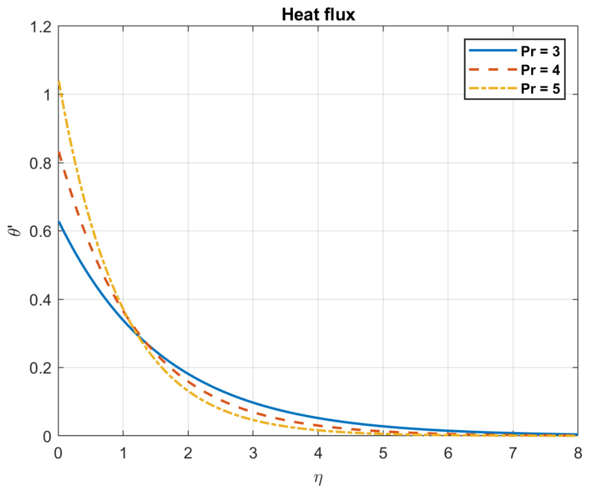
4.2. The Influence of Prandtl Number, P r

Examining the impact of Prandtl number, it is found that when P r values rise, so do the temperature, heat flow, nanoparticles, and bacterial density. This is because fluids with a high Prandtl number ( P r >> 1), such as oils or water, have a low heat conductivity in relation to their viscosity. Larger temperature gradients and a less uniform distribution of temperatures occur from the slower transport of heat. The heat flow is influenced by the Prandtl number. A fluid with a high Prandtl number will typically have a low heat flux for a given temperature difference. This is because a fluid with a low Prandtl number has reduced viscosity and better thermal conductivity, which enables it to transmit heat more effectively. The way that nanoparticles behave while suspended in a fluid is also influenced by the Prandtl number. This is due to the fact that nanoparticles can improve convective heat transfer by raising the fluid’s effective thermal conductivity, encouraging mixing, and facilitating fluid motion. Figure 3, Figure 4, Figure 5, Figure 6, Figure 7 and Figure 8 exhibit these observations.

4.3. The Influence of Magnetic Diffusivity η 0

Examining the impact of magnetic diffusivity, it is shown that an increase in η 0 values result in a decrease in both the magnetic field and nanofluid velocity. Because magnetotactic bacteria align with magnetic fields, they can affect the fluid flow patterns in bioconvection fluids. These bacteria’s alignment has the potential to alter the fluid’s effective viscosity and anisotropy, which will have an impact on the velocity field. The way the magnetic field interacts with the bacteria and modifies the fluid flow can be influenced by the medium’s magnetic diffusivity. Increased magnetic diffusivity can cause the magnetic field to dissipate more quickly, which will weaken the magnetotactic bacteria’s alignment. This might lead to a decrease in the effects of bioconvection and a weaker magnetic field modulation of the velocity field. The results are shown in Figure 9, Figure 10, Figure 11, Figure 12, Figure 13, Figure 14, Figure 15 and Figure 16.

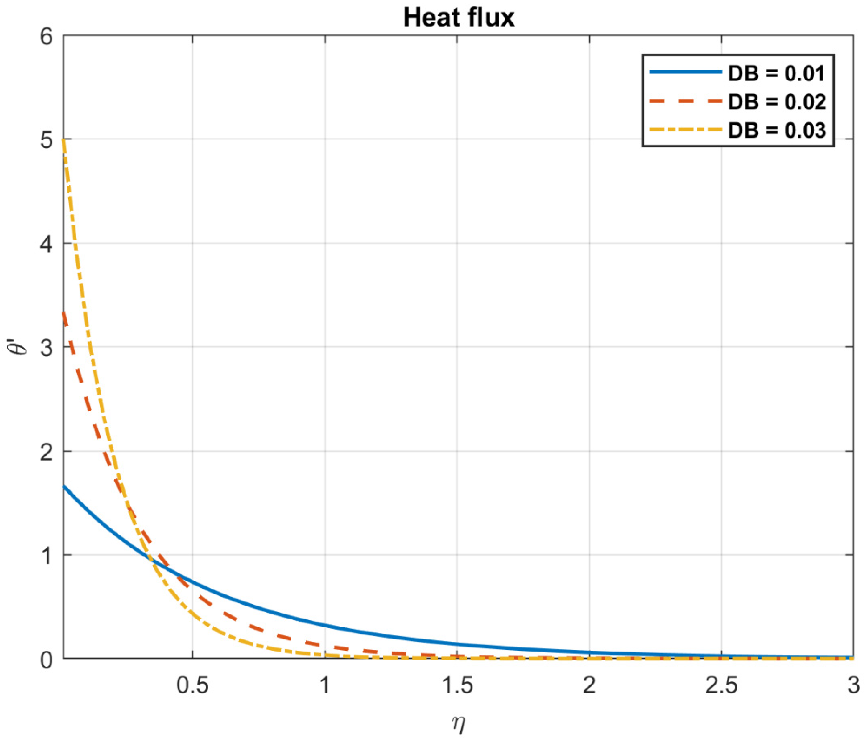
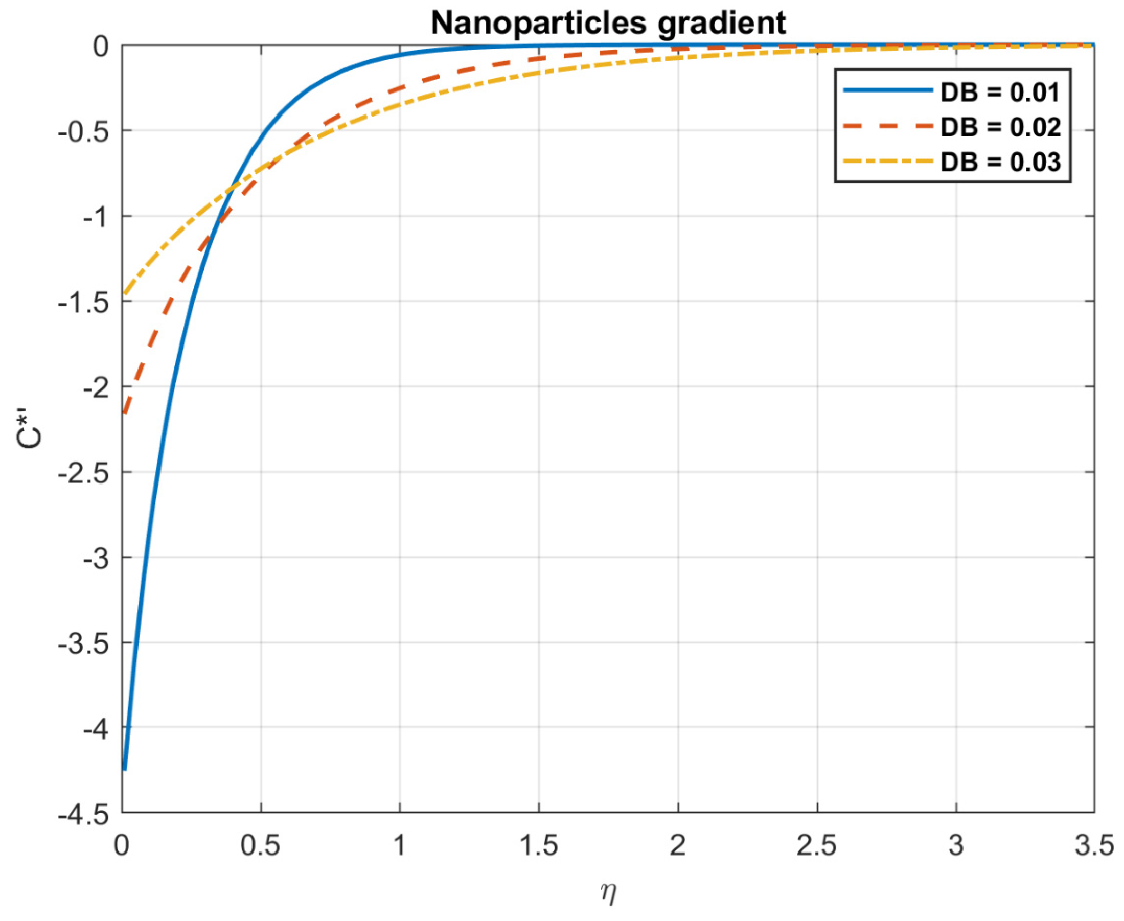
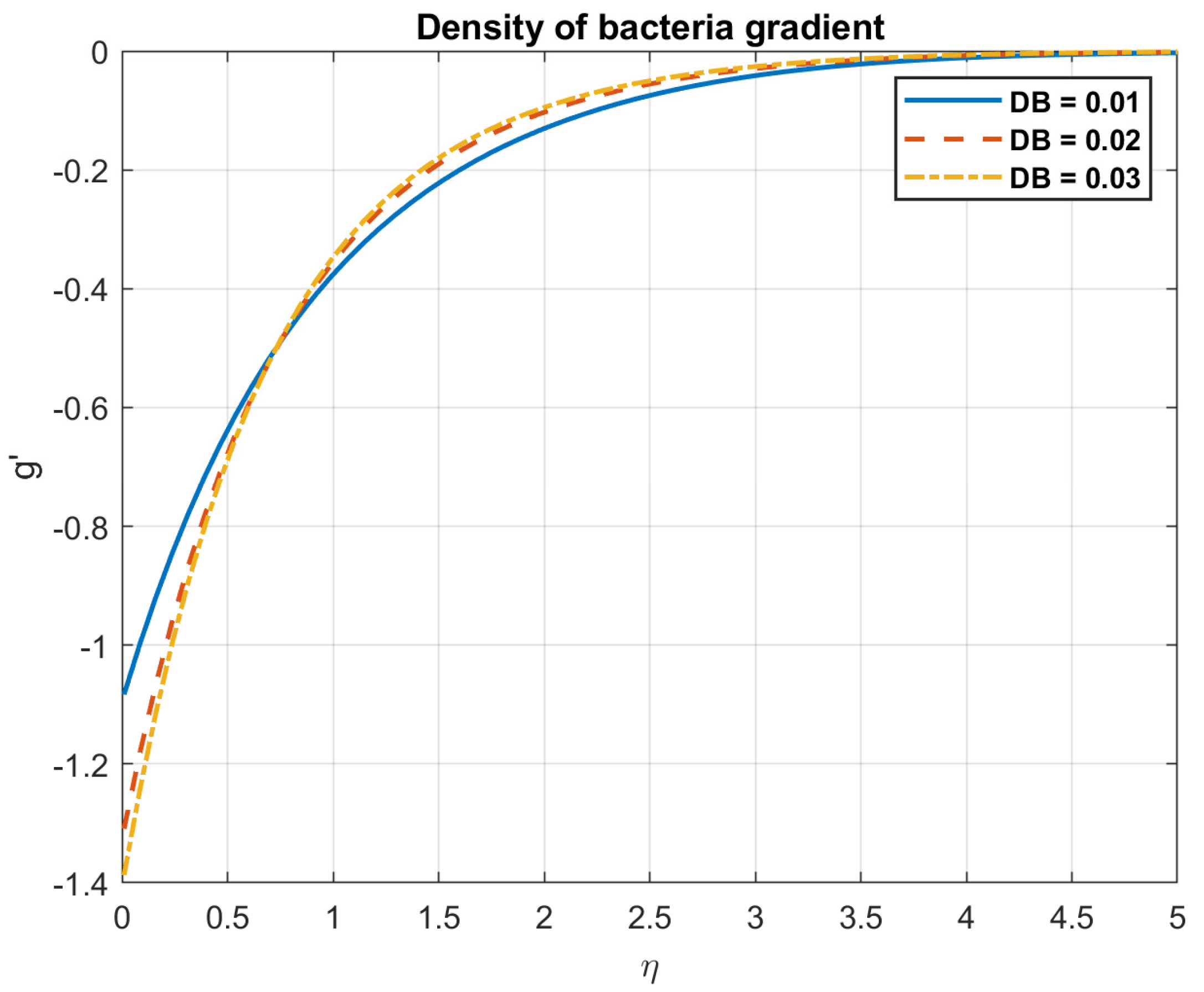
4.4. The Influence of Brownian Motion Coefficient, D B

Examining the impact of the Brownian motion coefficient demonstrates that when D B values rise, the temperature, heat flow, and bacterial density all drop. While the number of nanoparticles grows as D B values rise. This is due to the fact that the Brownian motion coefficient, which is inversely correlated with temperature, describes the random motion of particles floating in a fluid as a result of collisions with fluid molecules. As temperature increases, the random motion of fluid molecules becomes more energetic, leading to greater Brownian motion. The behavior of nanoparticles dispersed in bioconvection fluids is significantly influenced by the Brownian motion coefficient. Brownian motion disperses and mixes the nanoparticles in the fluid by causing them to move randomly. The diffusion and dispersion of nanoparticles are more noticeable with larger Brownian motion coefficients, and this can have an impact on the concentration gradients and general distribution of the particles in the fluid. This in turn affects how they interact with bacteria and the fluid around them. Figure 17, Figure 18, Figure 19, Figure 20, Figure 21 and Figure 22 demonstrate these observations.

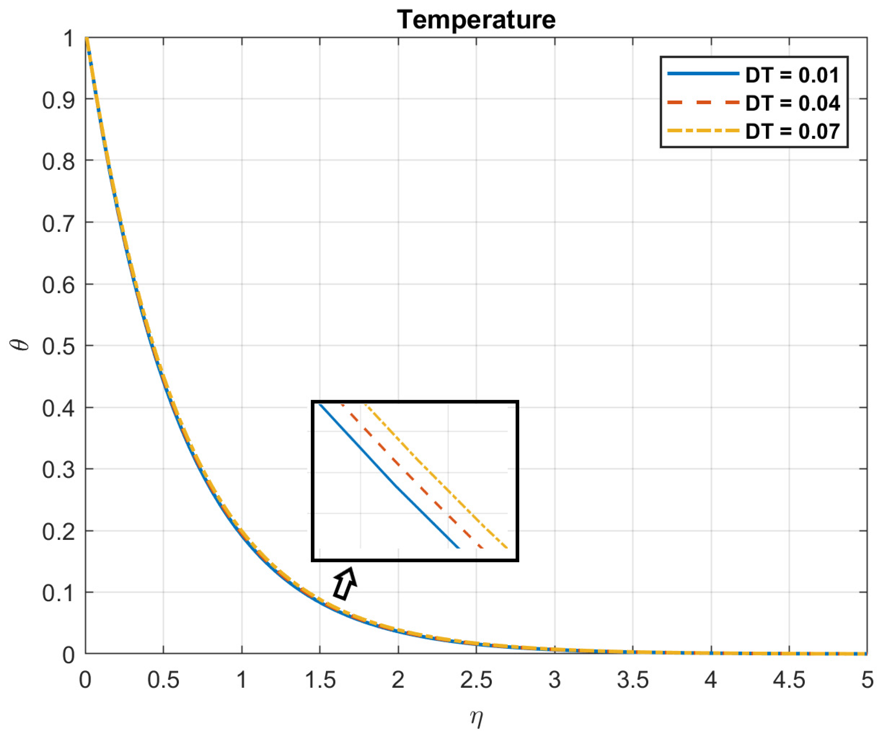
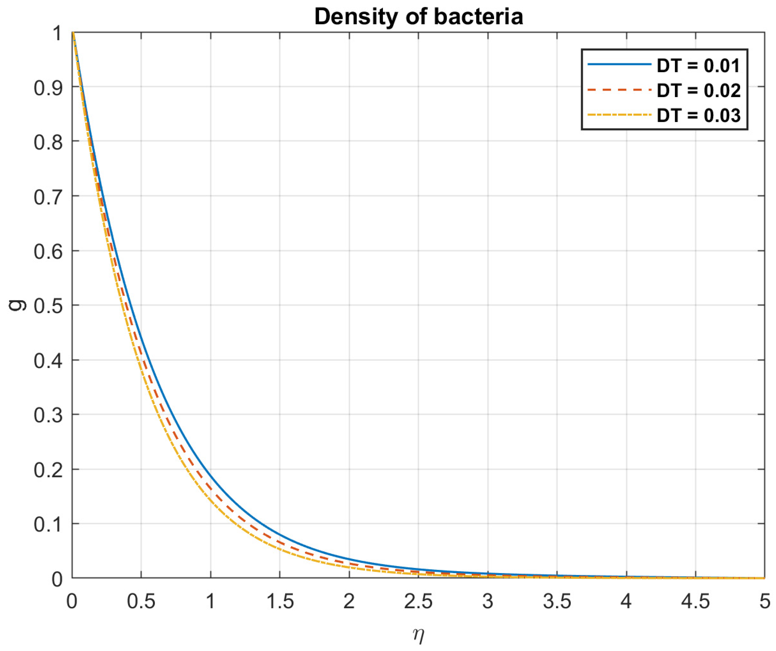
4.5. The Influence of Thermophoresis Diffusion Coefficient, D T

Examining the impact of the thermophoresis diffusion coefficient demonstrates that when D T values rise, so do the temperature, heat flow, and nanoparticles. However, when D T values rise, the density of bacteria falls. This is so because the movement of particles in a fluid due to a temperature gradient is called thermophoresis, and the thermophoresis diffusion coefficient is what defines it. It gauges how quickly particles move in response to temperature changes. The fluid’s particle concentration can have an impact on the thermophoresis diffusion coefficient. Particle interactions between individual particles and collective effects can affect the overall behavior of thermophoresis when concentrations of particles are elevated. Concentration gradients can be enhanced by a larger thermophoresis diffusion coefficient, which will accelerate particle migration toward areas of higher temperature. This may have an impact on the fluid’s particle density, heat flow, and temperature distribution. Figure 23, Figure 24, Figure 25, Figure 26, Figure 27 and Figure 28 exhibit these observations.

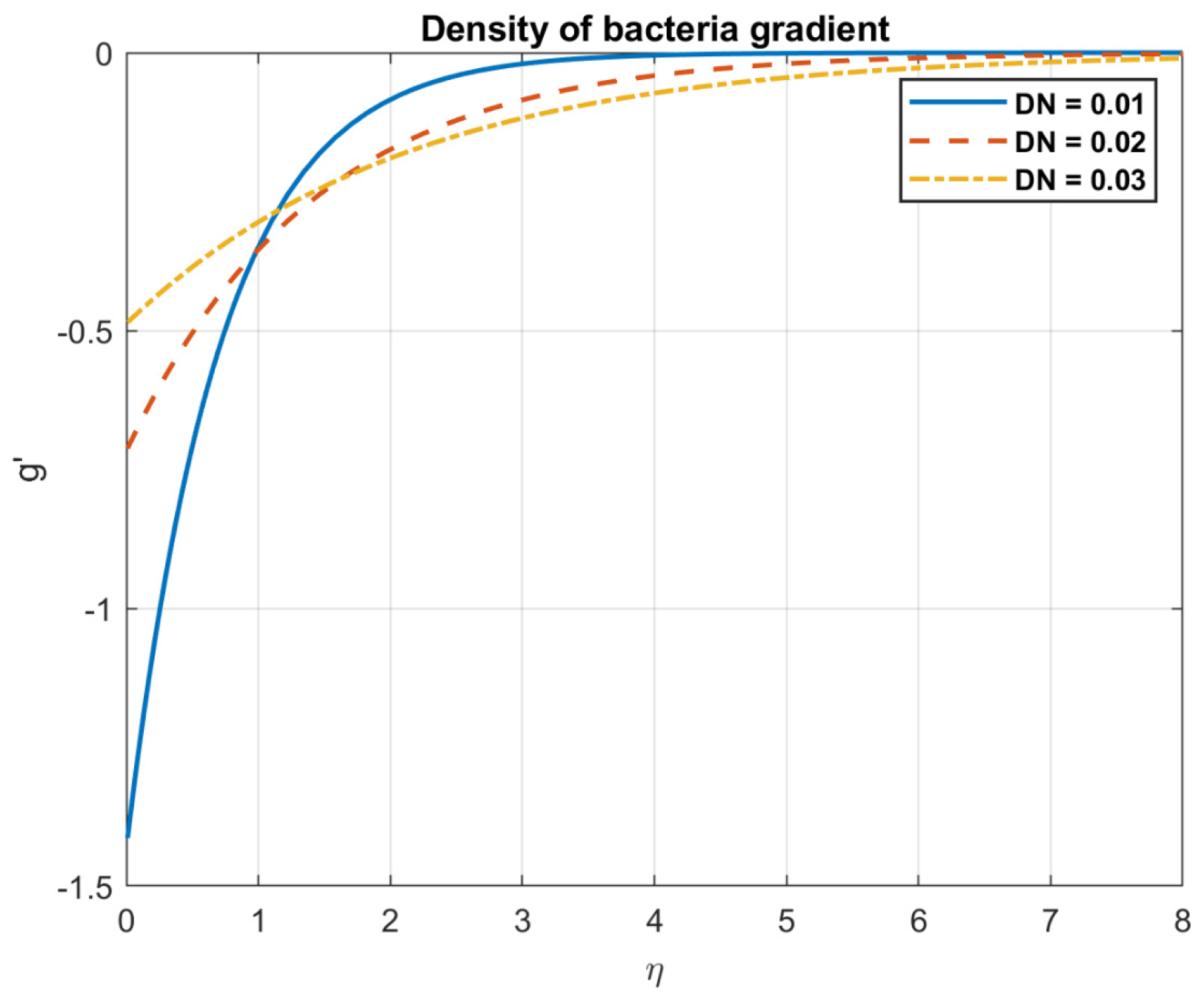
4.6. The Influence of Microorganism Diffusion Coefficient, D n

Examining the impact of the microbe diffusion coefficient demonstrates that as D n values rise, so does the bacterial density. This is because the rate at which bacteria proliferate and amalgamate within the fluid is determined by the diffusion coefficient. Because they may spread faster, bacteria with greater diffusion coefficients distribute more uniformly across the fluid volume. This could produce a general rise in the density of bacteria in the fluid due to the increased chances for contacts and interactions. In bioconvection fluids, it influences the dispersion and geographical distribution of microorganisms. Bacterial diffusion increases with a larger microorganism diffusion coefficient. The results are shown in Figure 29 and Figure 30.

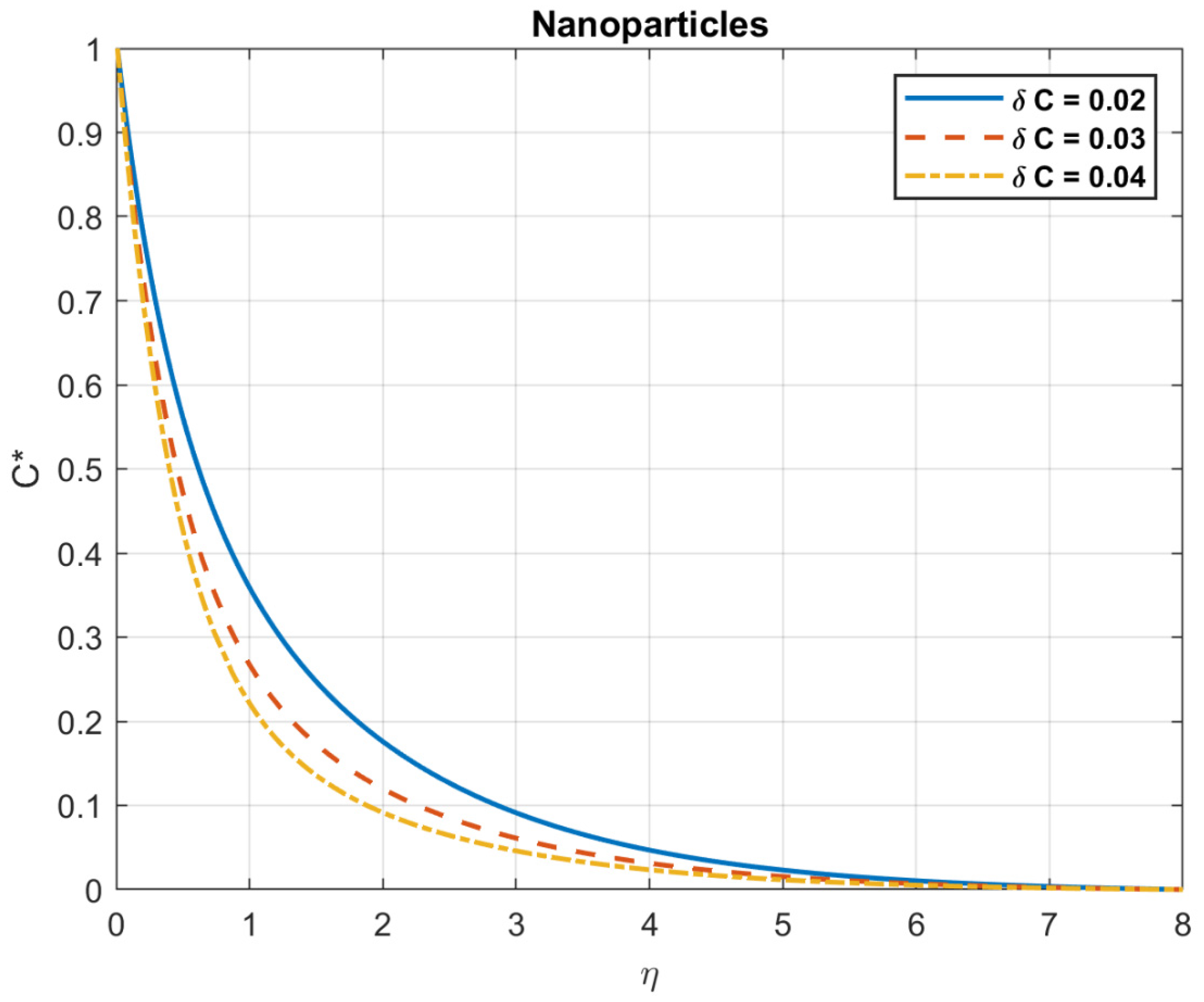
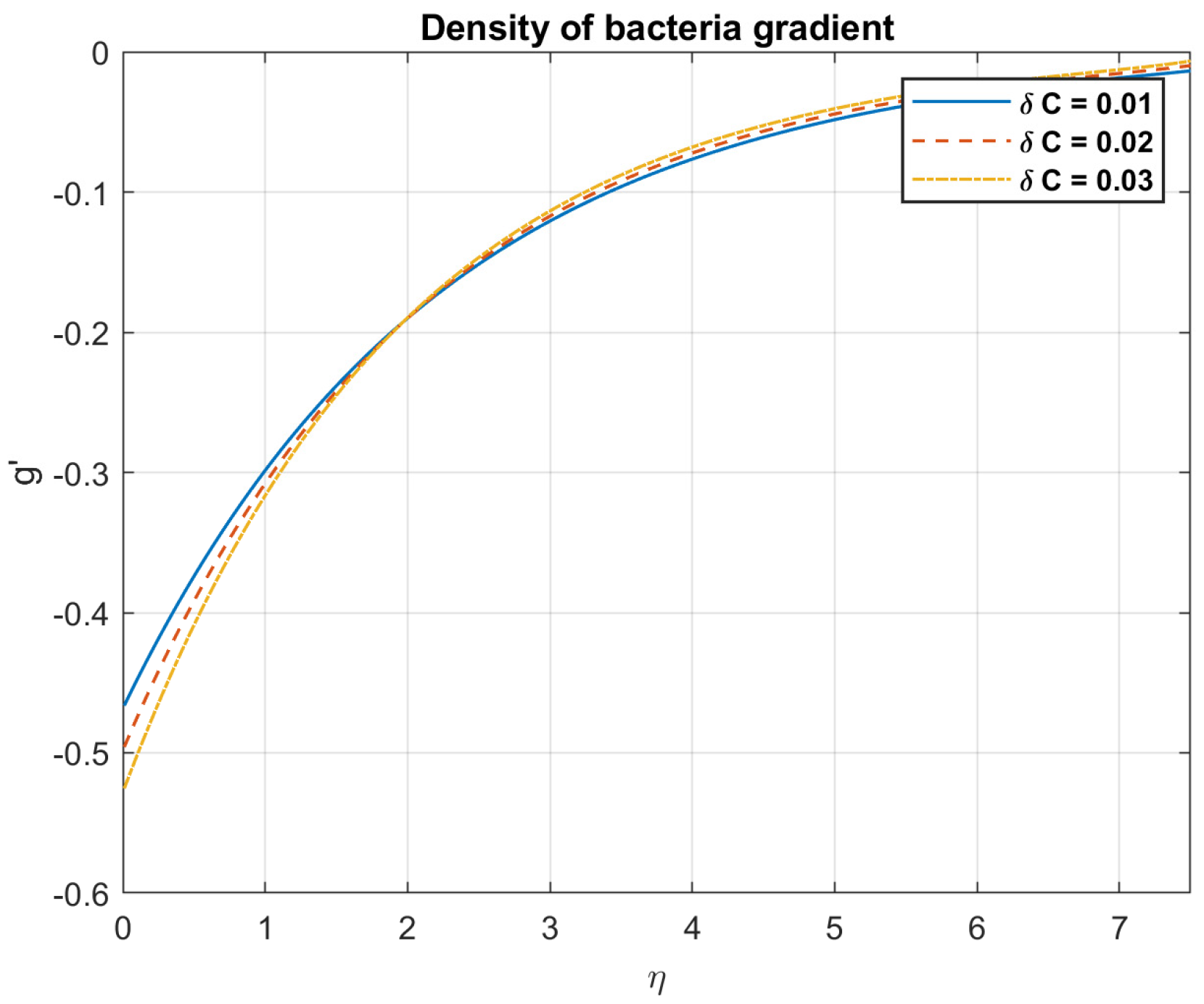
4.7. The Influence of Concentration Difference, δ c

Examining the impact of concentration differences, it is found that when δ c values rise, so do the temperature, heat flow, nanoparticles, and bacterial density. This is due to the fact that diffusion, which is fueled by concentration differences, is the net movement of particles from areas of greater concentration to regions of lower concentration. In the presence of a concentration gradient ( δ c ), the nanoparticles will tend to diffuse out and equalize the concentration distribution. Diffusion rate depends on a number of factors, including particle size, concentration, and fluid medium properties. The concentration difference diminishes with increasing diffusion over time. Buoyancy-driven flows can be produced by concentration differences. In bioconvection, for instance, microorganisms in a fluid travel toward warmer areas, causing density changes and upward flow. The results are shown in Figure 31, Figure 32, Figure 33, Figure 34, Figure 35 and Figure 36.

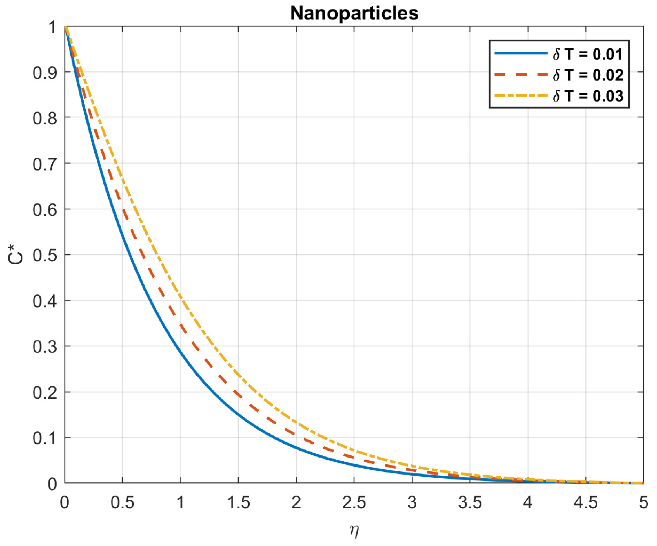
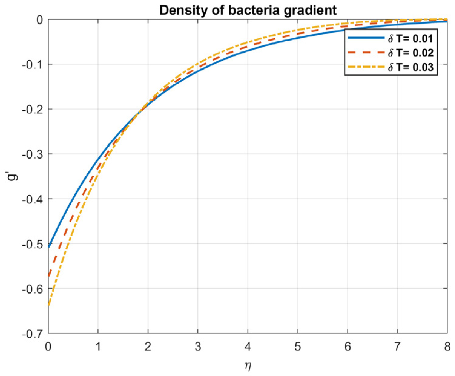
4.8. The Influence of Temperature Difference, δ t

Examining the impact of temperature variations, it is shown that while the density of bacteria decreases with increasing δ t values, the number of nanoparticles rises. This is due to the fact that variations in temperature can have an impact on the behavior of nanoparticles floating in a fluid. Nanoparticles may undergo thermophoretic mobility, also known as thermophoresis, in response to a temperature gradient. Temperature gradients cause thermophoresis, causing particles to migrate. Generally, particles go from warmer to colder environments. The amount and direction of the thermophoretic motion are determined by the fluid’s viscosity and heat conductivity, as well as the properties of the nanoparticles, including their size and surface charge. This phenomenon may affect the density and distribution of nanoparticles, causing them to scatter or collect in certain fluid areas. These findings are depicted in Figure 37, Figure 38, Figure 39 and Figure 40.

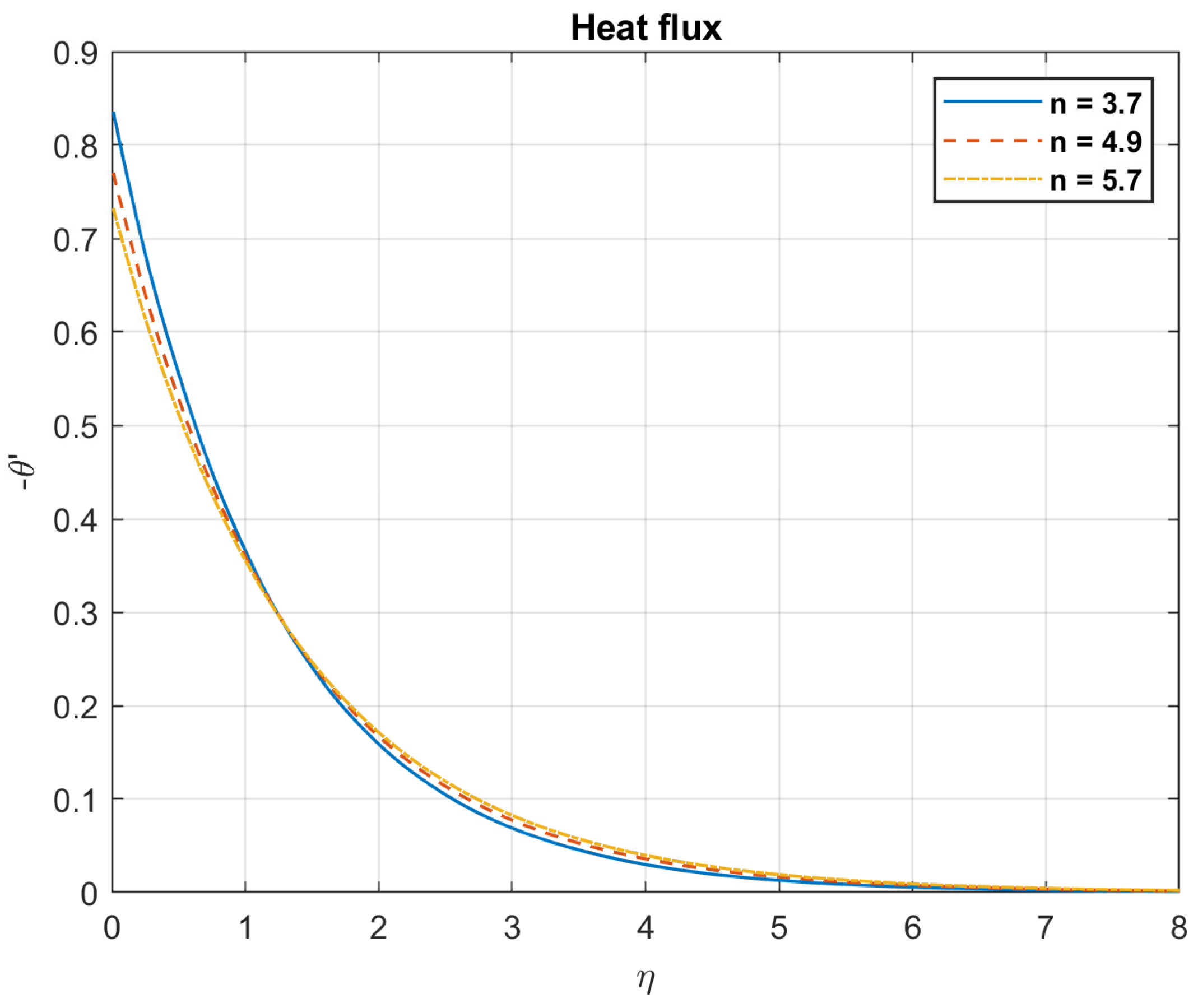
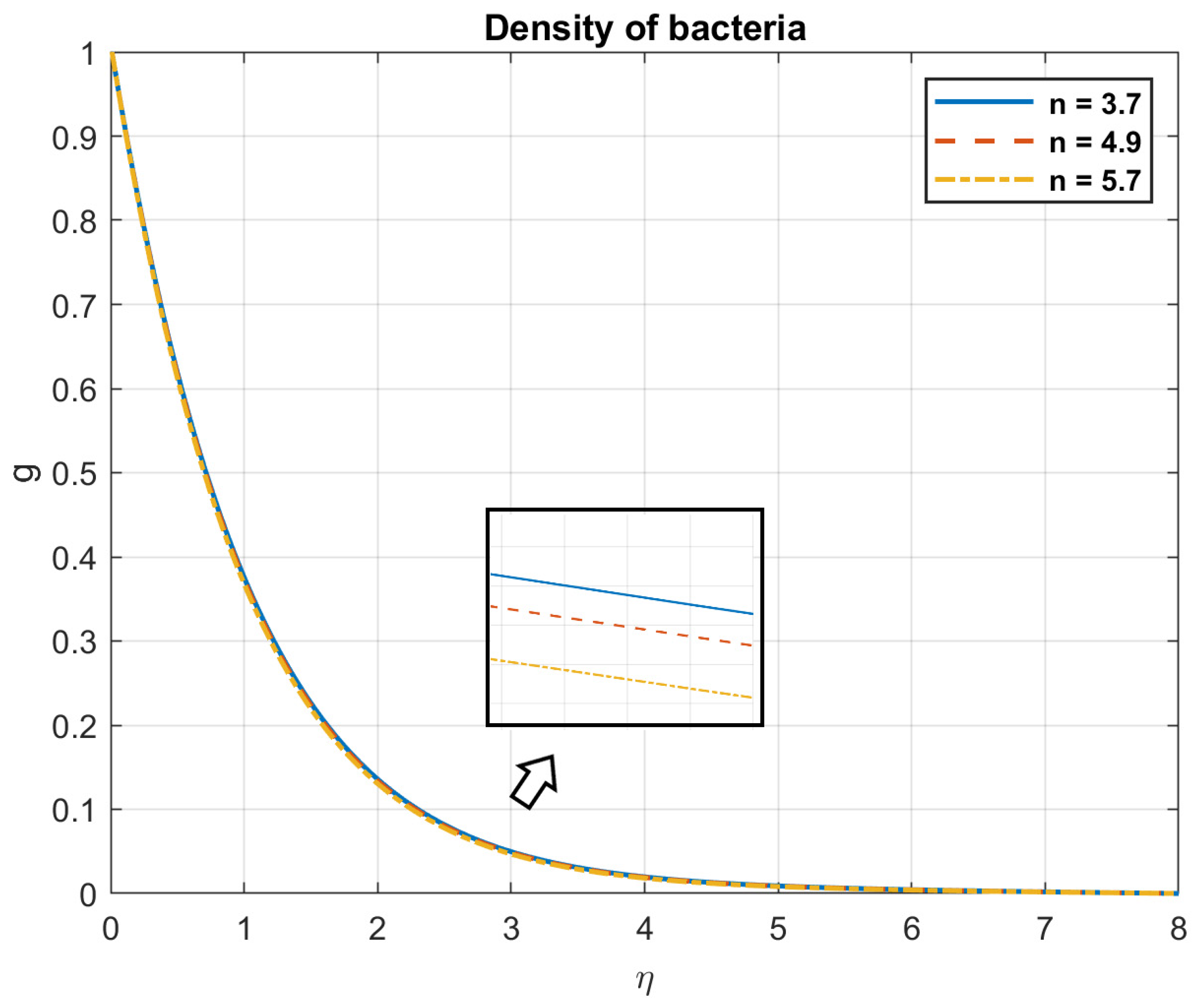
4.9. The Influence of Shape Factor, n

Examining how the form factor of the nanoparticle affects things shows that as n values increase, so does the density of both bacteria and nanoparticles. On the other hand, as n values grow, so do the temperature and heat flow. Because of their larger surface area, platelet nanoparticles with shape factor n = 5.7 adopt a higher temperature. Figure 41, Figure 42, Figure 43, Figure 44, Figure 45 and Figure 46 show these results.

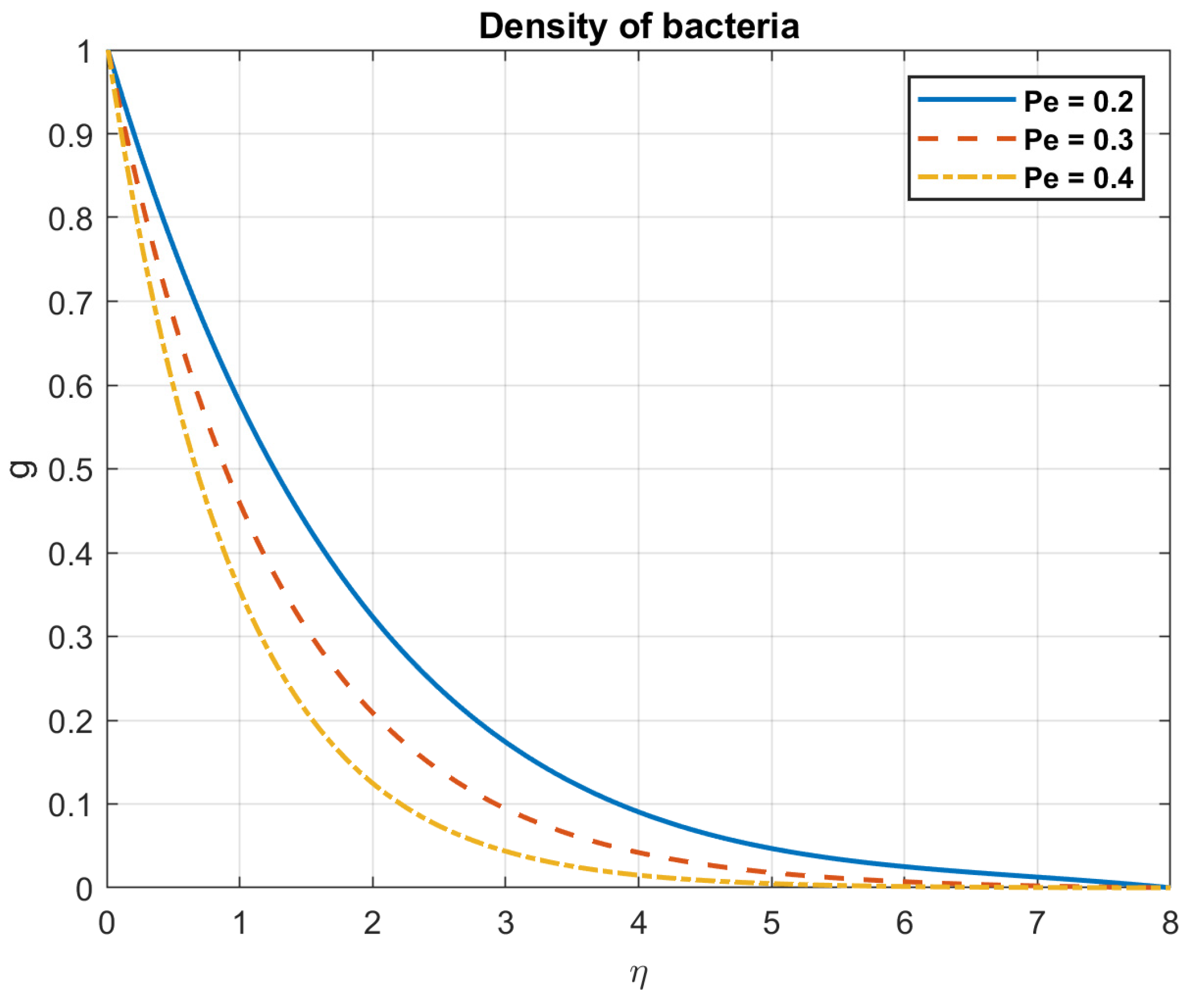
4.10. The Influence of Bioconvection Peclet Number, P e

Examining the impact of bioconvection Peclet number indicates that when Pe values increase, the density of bacteria decreases. A rapid reduction in thickness is observed in motile bacteria when the number of Peclets increases. Stated differently, the reduction in the thickness of the motile bacteria and the subsequent decrease in the microorganisms’ dispersion was likely due to the strengthening of the Peclet number. For motile bacteria, this results in a drooping of the thickness and limit layer thickness due to an increase in Pe. Greater Peclet numbers indicate that diffusion is less important than advection. This effectively lowers the local density of bacteria by limiting their tendency to disperse and uniformly inhabit the area. Figure 47 and Figure 48 illustrate these results.

5. Conclusions

The unsteady electrically conducting hybrid nanofluid (Fe3O4-Cu/water) including viscous and gyrotactic microorganisms near the stagnation point of a laminar-mixed convection incompressible flow. Additionally, magnetic field effects from the outside and from within, as well as hybrid nanofluid flow across a horizontal porous stretched sheet, The analysis of the effects of several parameters served as the inspiration for the current study, including Prandtl number, P r , magnetic diffusivity, η 0 , shape factor,   n , microorganism diffusion coefficient, D n , Brownian motion coefficient, D B , thermophoresis diffusion coefficient,   D T , bioconvection Peclet number, P e , temperature difference,   δ t , and concentration difference,   δ c .
  • The temperature, heat flow, nanoparticles, and bacterial density all drop when P r values rise;
  • Examining the impact of magnetic diffusivity, it is shown that an increase in η 0 values result in a decrease in both the magnetic field and nanofluid velocity;
  • The temperature, heat flow, and bacterial density all drop as D B values rise;
  • The temperature, heat flow, and nanoparticles all rise when D T values rise;
  • Examining how the microbe diffusion coefficient affects things shows that as D n values rise, so does the density of bacteria;
  • Examining the effect of concentration difference indicates that when δ c values rise, the temperature, heat flow, bacterial density, and nanoparticles all decrease;
  • Examining the impact of temperature variations shows that when δ t values rise, the number of nanoparticles increases while the density of bacteria decreases;
  • Examining the impact of the nanoparticle shape factor demonstrates that as n values increase, so does the density of both nanoparticles and bacteria;
  • Examining the effects of bioconvection Peclet number indicates that an increase in P e values results in a decrease in bacterial density.

Author Contributions

Conceptualization, S.M.M. and A.S.R.; methodology, S.M.M., A.S.R. and E.H.N.; software, A.S.R. and E.H.N.; validation, E.H.N.; writing—original draft preparation, E.H.N. and A.S.R.; writing—review and editing, E.H.N., A.S.R. and S.M.M.; visualization, E.H.N.; supervision, S.M.M. and A.S.R. All authors have read and agreed to the published version of the manuscript.

Funding

This research received no external funding.

Data Availability Statement

No new data were created or analyzed in this study. Data sharing is not applicable to this article.

Conflicts of Interest

The authors declare no conflict of interest.

Nomenclature

Latin characters
u , v , w Components of velocity
u w , v w Stretching velocity
H 1 , H 2 Components of magnetic field
H 1 * , H 2 * Stretching magnetic field
x , y , z , t Independent variables
w 0 Constant
H 1 e , H 2 e External magnetic flux
k * Mean absorption coefficient
g Acceleration due to gravity
k h n f Thermal conductivity of hybrid nanofluid
D B Brownian diffusion coefficient
D T Thermophoresis diffusion coefficient
T Temperature of nanoparticles
T w Temperature at wall
T Ambient temperature
c Concentration of nanoparticles
c w Concentration at wall
c Ambient concentration
N Microorganisms’ concentration
N w Microorganisms at wall
N Ambient microorganisms
P r Prandtl number
Q Volumetric rate of heat generation/absorption
n Shape factor
w c Cell swimming speed
b * Thermal relaxation constant
P e Bioconvection Peclet number
D N Microorganism diffusion coefficient
V 0 Suction/injection velocity
δ t Temperature difference
δ c Concentration difference
K s , Q s Differential coefficient functions
S System variables
G Group structure
S i Original dependent variables of the system
c 1 , c 2 , c 3 , , , , Constants
Greek characters
μ e Magnetic permeability
ρ h n f Density of hybrid nanofluid
μ h n f Viscosity of hybrid nanofluid
η 0 Magnetic diffusivity
ρ m Density of microorganisms
ρ f Density of base fluid
β Magnetic field parameter
ρ c p h n f Volumetric heat capacity of hybrid nanofluid
η Similarity variable

References

  1. Ali, A.; Sarkar, S.; Das, S.; Jana, R.N. Investigation of cattaneo–christov double diffusions theory in bioconvective slip flow of radiated magneto-cross-nanomaterial over stretching cylinder/plate with activation energy. Int. J. Appl. Comput. Math. 2021, 7, 208. [Google Scholar] [CrossRef]
  2. Alwatban, A.M.; Khan, S.U.; Waqas, H.; Tlili, I. Interaction of Wu’s slip features in bioconvection of Eyring Powell nanoparticles with activation energy. Processes 2019, 7, 859. [Google Scholar] [CrossRef]
  3. Biswas, N.; Mandal, D.K.; Manna, N.K.; Benim, A.C. Enhanced energy and mass transport dynamics in a thermo-magneto-bioconvective porous system containing oxytactic bacteria and nanoparticles: Cleaner energy application. Energy 2023, 263, 125775. [Google Scholar] [CrossRef]
  4. Dawar, A.; Saeed, A.; Islam, S.; Shah, Z.; Kumam, W.; Kumam, P. Electromagnetohydrodynamic bioconvective flow of binary fluid containing nanoparticles and gyrotactic microorganisms through a stratified stretching sheet. Sci. Rep. 2021, 11, 23159. [Google Scholar] [CrossRef] [PubMed]
  5. Ghadikolaei, S.; Hosseinzadeh, K.; Ganji, D. Investigation on three dimensional squeezing flow of mixture base fluid (ethylene glycol-water) suspended by hybrid nanoparticle (Fe3O4-Ag) dependent on shape factor. J. Mol. Liquids 2018, 262, 376–388. [Google Scholar] [CrossRef]
  6. Ghadikolaei, S.; Hosseinzadeh, K.; Ganji, D. Investigation on ethylene glycol-water mixture fluid suspend by hybrid nanoparticles (TiO2-CuO) over rotating cone with considering nanoparticles shape factor. J. Mol. Liquids 2018, 272, 226–236. [Google Scholar] [CrossRef]
  7. Hosseinzadeh, K.; Asadi, A.; Mogharrebi, A.; Ermia Azari, M.; Ganji, D. Investigation of mixture fluid suspended by hybrid nanoparticles over vertical cylinder by considering shape factor effect. J. Therm. Anal. Calorim. 2021, 143, 1081–1095. [Google Scholar] [CrossRef]
  8. Hosseinzadeh, K.; Roghani, S.; Mogharrebi, A.; Asadi, A.; Ganji, D. Optimization of hybrid nanoparticles with mixture fluid flow in an octagonal porous medium by effect of radiation and magnetic field. J. Therm. Anal. Calorim. 2021, 143, 1413–1424. [Google Scholar] [CrossRef]
  9. Hosseinzadeh, K.; Salehi, S.; Mardani, M.; Mahmoudi, F.; Waqas, M.; Ganji, D. Investigation of nano-Bioconvective fluid motile microorganism and nanoparticle flow by considering MHD and thermal radiation. Inform. Med. Unlocked 2020, 21, 100462. [Google Scholar] [CrossRef]
  10. Khan, N.S.; Shah, Q.; Sohail, A.; Ullah, Z.; Kaewkhao, A.; Kumam, P.; Zubair, S.; Ullah, N.; Thounthong, P. Rotating flow assessment of magnetized mixture fluid suspended with hybrid nanoparticles and chemical reactions of species. Sci. Rep. 2021, 11, 11277. [Google Scholar] [CrossRef]
  11. Koriko, O.K.; Shah, N.A.; Saleem, S.; Chung, J.D.; Omowaye, A.J.; Oreyeni, T. Exploration of bioconvection flow of MHD thixotropic nanofluid past a vertical surface coexisting with both nanoparticles and gyrotactic microorganisms. Sci. Rep. 2021, 11, 16627. [Google Scholar] [CrossRef]
  12. Kuznetsov, A. The onset of nanofluid bioconvection in a suspension containing both nanoparticles and gyrotactic microorganisms. Int. Commun. Heat Mass Transf. 2010, 37, 1421–1425. [Google Scholar] [CrossRef]
  13. Mahanthesh, B.; Thriveni, K. Significance of inclined magnetic field on nano-bioconvection with nonlinear thermal radiation and exponential space based heat source: A sensitivity analysis. Eur. Phys. J. Spec. Top. 2021, 230, 1487–1501. [Google Scholar] [CrossRef]
  14. Mohamed, K.; Ismail, T.; Nourreddine, N.; Mohamed Rafik, S. Analytical study of nano-bioconvective flow in a horizontal channel using Adomian decomposition method. J. Comput. Appl. Res. Mech. Eng. 2020, 9, 245–258. [Google Scholar]
  15. Moradi, M.R.; Hosseinzadeh, K.; Hasibi, A.; Domiri Ganji, D. Hydrothermal study on nano-bioconvective fluid flow over a vertical plate under the effect of magnetic field. Numer. Heat Transf. Part B Fundam. 2023, 1–15. [Google Scholar] [CrossRef]
  16. Nawaz, M. Role of hybrid nanoparticles in thermal performance of Sutterby fluid, the ethylene glycol. Phys. A Stat. Mech. Its Applic. 2020, 537, 122447. [Google Scholar] [CrossRef]
  17. Nawaz, M.; Nazir, U.; Saleem, S.; Alharbi, S.O. An enhancement of thermal performance of ethylene glycol by nano and hybrid nanoparticles. Phys. A Stat. Mech. Its Applic. 2020, 551, 124527. [Google Scholar] [CrossRef]
  18. Nazir, U.; Nawaz, M.; Alharbi, S.O. Thermal performance of magnetohydrodynamic complex fluid using nano and hybrid nanoparticles. Phys. A Stat. Mech. Its Applic. 2020, 553, 124345. [Google Scholar] [CrossRef]
  19. Rana, B.; Arifuzzaman, S.; Islam, S.; Reza-E-Rabbi, S.; Al-Mamun, A.; Mazumder, M.; Roy, K.C.; Khan, M.S. Swimming of microbes in blood flow of nano-bioconvective Williamson fluid. Therm. Sci. Eng. Prog. 2021, 25, 101018. [Google Scholar] [CrossRef]
  20. Aziz, S.; Kolsi, L.; Ahmad, I.; Al-Turjman, F.; Omri, M.; Khan, S.U. Thermal stability and bioconvection investigation for couple stress nanofluid due to a three-dimensional accelerated frame. Waves Random Complex Media 2022, 1–22. [Google Scholar] [CrossRef]
  21. Mansour, M.A.; Rashad, A.M.; Mallikarjuna, B.; Hussein, A.K.; Aichouni, M.; Kolsi, L. MHD mixed bioconvection in a square porous cavity filled by gyrotactic microorganisms. Int. J. Heat Technol. 2019, 37, 433–445. [Google Scholar] [CrossRef]
  22. Ghachem, K.; Al-Khaled, K.; Khan, S.U.; Alwadai, N.; Alshammari, B.M.; Kolsi, L.; Chammam, W.; Almuqrin, M. An unsteady bioconvective non-Newtonian nanofluid model with variable thermal properties and modified heat flux framework. Int. J. Modern Phys. B 2023, 9, 2450202. [Google Scholar] [CrossRef]
  23. Almeshaal, M.A.; Palaniappan, M.; Kolsi, L. Significance of induced magnetic force for bioconvective transport of thixotropic nanofluid with variable thermal conductivity. Int. J. Modern Phys. B 2023, 37, 2350298. [Google Scholar] [CrossRef]
  24. Rana, P.; Makkar, V.; Gupta, G. Finite element study of bio-convective Stefan blowing Ag-MgO/water hybrid nanofluid induced by stretching cylinder utilizing non-Fourier and non-Fick’s laws. Nanomaterials 2021, 11, 1735. [Google Scholar] [CrossRef] [PubMed]
  25. Bees, M.A.; Croze, O.A. Mathematics for streamlined biofuel production from unicellular algae. Biofuels 2014, 5, 53–65. [Google Scholar] [CrossRef]
  26. Saleem, S.; Rafiq, H.; Al-Qahtani, A.; El-Aziz, M.A.; Malik, M.; Animasaun, I. Magneto Jeffrey nanofluid bioconvection over a rotating vertical cone due to gyrotactic microorganism. Math. Probl. Eng. 2019, 2019, 3478037. [Google Scholar] [CrossRef]
  27. Adhikari, R.; Das, S. Biological transmission in a magnetized reactive Casson–Maxwell nanofluid over a tilted stretchy cylinder in an entropy framework. Chin. J. Phys. 2023, 86, 194–226. [Google Scholar] [CrossRef]
  28. Hazarika, S.; Ahmed, S. Physical Insights on Bio-Convection in Prandtl Nanofluid over an Inclined Stretching Sheet in Non-Darcy Medium: Numerical Simulation. Sci. Iran. 2023, in press.
  29. Ge-JiLe, H.; Waqas, H.; Khan, S.U.; Khan, M.I.; Farooq, S.; Hussain, S. Three-dimensional radiative bioconvective flow of a sisko nanofluid with motile microorganisms. Coatings 2021, 11, 335. [Google Scholar] [CrossRef]
  30. Datta, T.; Rajoria, A.; Sk, M.T. Bioconvective Study on Flow Analysis of the Mhd Falkner-Skan Flow of Eyring-Powell Nanofluid with Gyrotatic Microorganism Past A Wedge. J. Biol. Syst. 2016, 24, 1–21. [Google Scholar]
  31. Alsheekhhussain, Z.; Moaddy, K.; Shah, R.; Alshammari, S.; Alshammari, M.; Al-Sawalha, M.M.; Alderremy, A.A. Extension of the Optimal Auxiliary Function Method to Solve the System of a Fractional-Order Whitham–Broer–Kaup Equation. Fractal Fract. 2023, 8, 1. [Google Scholar] [CrossRef]
  32. Al-Sawalha, M.M.; Mukhtar, S.; Shah, R.; Ganie, A.H.; Moaddy, K. Solitary Waves Propagation Analysis in Nonlinear Dynamical System of Fractional Coupled Boussinesq-Whitham-Broer-Kaup Equation. Fract. Fract. 2023, 7, 889. [Google Scholar] [CrossRef]
  33. Al-Sawalha, M.M.; Yasmin, H.; Shah, R.; Ganie, A.H.; Moaddy, K. Unraveling the Dynamics of Singular Stochastic Solitons in Stochastic Fractional Kuramoto–Sivashinsky Equation. Fract. Fract. 2023, 7, 753. [Google Scholar] [CrossRef]
  34. Salehi, S.; Nori, A.; Hosseinzadeh, K.; Ganji, D.D. Hydrothermal analysis of MHD squeezing mixture fluid suspended by hybrid nanoparticles between two parallel plates. Case Stud. Therm. Eng. 2020, 21, 100650. [Google Scholar] [CrossRef]
  35. Uddin, M.J.; Rana, P.; Gupta, S.; Uddin, M.N. Bio-nanoconvective Micropolar Fluid Flow in a Darcy Porous Medium Past a Cone with Second-Order Slips and Stefan Blowing: FEM Solution. Iran. J. Sci. Technol. Trans. Mech. Eng. 2023, 47, 1–15. [Google Scholar] [CrossRef]
  36. Uddin, M.J.; Kabir, M.N.; Alginahi, Y.; Bég, O.A. Numerical solution of bio-nano-convection transport from a horizontal plate with blowing and multiple slip effects. Proc. Inst. Mech. Eng. Part C J. Mech. Eng. Sci. 2019, 233, 6910–6927. [Google Scholar] [CrossRef]
  37. Waqas, H.; Farooq, U.; Bhatti, M.M.; Hussain, S. Magnetized bioconvection flow of Sutterby fluid characterized by the suspension of nanoparticles across a wedge with activation energy. ZAMM-J. Appl. Math. Mech./Z. Für Angew. Math. Mech. 2021, 101, e202000349. [Google Scholar] [CrossRef]
  38. Waqas, H.; Khan, S.U.; Hassan, M.; Bhatti, M.M.; Imran, M. Analysis on the bioconvection flow of modified second-grade nanofluid containing gyrotactic microorganisms and nanoparticles. J. Mol. Liq. 2019, 291, 111231. [Google Scholar] [CrossRef]
  39. Yook, S.J.; Raju, C.S.K.; Almutairi, B.; Mamatha, S.U.; Shah, N.A.; Eldin, S.M. Heat and momentum diffusion of ternary hybrid nanoparticles in a channel with dissimilar permeability’s and moving porous walls: A Multi-linear regression. Case Stud. Therm. Eng. 2023, 47, 103133. [Google Scholar] [CrossRef]
  40. Zuhra, S.; Khan, N.S.; Shah, Z.; Islam, S.; Bonyah, E. Simulation of bioconvection in the suspension of second grade nanofluid containing nanoparticles and gyrotactic microorganisms. Aip Adv. 2018, 8, 105210. [Google Scholar] [CrossRef]
  41. Morgan, A.J.A. The reduction by one of the number of independent variables in some systems of partial differential equations. Q. J. Math. 1952, 3, 250–259. [Google Scholar] [CrossRef]
  42. Mabrouk, S.M.; Rashed, A.S. Analysis of (3 + 1)-dimensional Boiti—Leon—Manna–Pempinelli equation via Lax pair investigation and group transformation method. Comput. Math. Appl. 2017, 74, 2546–2556. [Google Scholar] [CrossRef]
  43. Saleh, R.; Kassem, M.; Mabrouk, S. Exact solutions of Calgero-Bogoyavlenskii-Schiff equation using the singular manifold method after Lie reductions. MMA Math. Methods Appl. Sci. 2017, 40, 5851–5862. [Google Scholar] [CrossRef]
  44. Rashed, A.S.; Kassem, M.M. Group analysis for natural convection from a vertical plate. J. Comput. Appl. Math. 2008, 222, 392–403. [Google Scholar] [CrossRef]
  45. Mabrouk, S.; Kassem, M. Group similarity solutions of (2 + 1) Boiti-Leon-Manna-Pempinelli Lax pair. ASEJ Ain Shams Eng. J. 2014, 5, 227–235. [Google Scholar] [CrossRef]
  46. Mabrouk, S.; Kassem, M.; Abd-el-Malek, M. Group similarity solutions of the lax pair for a generalized Hirota-Satsuma equation. Appl. Math. Comput. 2013, 219, 7882–7890. [Google Scholar] [CrossRef]
  47. Kassem, M.M.; Rashed, A.S. Group solution of a time dependent chemical convective process. Appl. Math. Comput. 2009, 215, 1671–1684. [Google Scholar] [CrossRef]
  48. Rashed, A.S.; Mahmoud, T.; Kassem, M. Analysis of homogeneous steady state nanofluid surrounding cylindrical solid pipes. Egypt. J. Eng. Sci. Technol. 2020, 31, 71–82. [Google Scholar] [CrossRef]
  49. Alshomrani, A.S.; Ullah, M.Z.; Baleanu, D. Importance of multiple slips on bioconvection flow of cross nanofluid past a wedge with gyrotactic motile microorganisms. Case Stud. Therm. Eng. 2020, 22, 100798. [Google Scholar] [CrossRef]
Figure 1. Physical representation of the problem.
Computation 12 00017 g001
Figure 2. Prandtl number P r , temperature comparison; dashed lines for our study, solid for H. Waqas et al. [49].
Computation 12 00017 g002
Figure 3. The impact of Prandtl number P r , on temperature.
Computation 12 00017 g003
Figure 4. The impact of Prandtl number P r , on heat flux.
Computation 12 00017 g004
Figure 5. The impact of Prandtl number P r , on nanoparticles.
Computation 12 00017 g005
Figure 6. The impact of Prandtl number P r , on nanoparticles gradient.
Computation 12 00017 g006
Figure 7. The impact of Prandtl number P r , on density of bacteria.
Computation 12 00017 g007
Figure 8. The impact of Prandtl number P r , on density gradient of bacteria.
Computation 12 00017 g008
Figure 9. The impact of magnetic diffusivity η 0 , on magnetic field along x-axis.
Computation 12 00017 g009
Figure 10. The impact of magnetic diffusivity η 0 , on magnetic field gradient along x-axis.
Computation 12 00017 g010
Figure 11. The impact of magnetic diffusivity η 0 , on magnetic field along y-axis.
Computation 12 00017 g011
Figure 12. The impact of magnetic diffusivity η 0 , on magnetic field gradient along y-axis.
Computation 12 00017 g012
Figure 13. The impact of magnetic diffusivity η 0 , on velocity in x-direction.
Computation 12 00017 g013
Figure 14. The impact of magnetic diffusivity η 0 , on shear in x-direction.
Computation 12 00017 g014
Figure 15. The impact of magnetic diffusivity η 0 , on velocity in y-direction.
Computation 12 00017 g015
Figure 16. The impact of magnetic diffusivity η 0 , on shear in y-direction.
Computation 12 00017 g016
Figure 17. The impact of Brownian motion coefficient, D B , on temperature.
Computation 12 00017 g017
Figure 18. The impact of Brownian motion coefficient, D B , on heat flux.
Computation 12 00017 g018
Figure 19. The impact of Brownian motion coefficient, D B , on nanoparticles.
Computation 12 00017 g019
Figure 20. The impact of Brownian motion coefficient, D B , on nanoparticles gradient.
Computation 12 00017 g020
Figure 21. The impact of Brownian motion coefficient, D B , on density of bacteria.
Computation 12 00017 g021
Figure 22. The impact of Brownian motion coefficient, D B , on density of bacteria gradient.
Computation 12 00017 g022
Figure 23. The impact of thermophoresis diffusion coefficient, D T , on temperature.
Computation 12 00017 g023
Figure 24. The impact of thermophoresis diffusion coefficient, D T , on heat flux.
Computation 12 00017 g024
Figure 25. The impact of thermophoresis diffusion coefficient, D T , on nanoparticles.
Computation 12 00017 g025
Figure 26. The impact of thermophoresis diffusion coefficient, D T , on nanoparticles gradient.
Computation 12 00017 g026
Figure 27. The impact of thermophoresis diffusion coefficient, D T , on density of bacteria.
Computation 12 00017 g027
Figure 28. The impact of thermophoresis diffusion coefficient, D T , on density of bacteria gradient.
Computation 12 00017 g028
Figure 29. The impact of microorganism diffusion coefficient, D n , on density of bacteria.
Computation 12 00017 g029
Figure 30. The impact of microorganism diffusion coefficient, D n , on density of bacteria gradient.
Computation 12 00017 g030
Figure 31. The impact of concentration difference, δ c , on temperature.
Computation 12 00017 g031
Figure 32. The impact of concentration difference, δ c , on heat flux.
Computation 12 00017 g032
Figure 33. The impact of concentration difference, δ c , on nanoparticles.
Computation 12 00017 g033
Figure 34. The impact of concentration difference, δ c , on nanoparticles gradient.
Computation 12 00017 g034
Figure 35. The impact of concentration difference, δ c , on density of bacteria.
Computation 12 00017 g035
Figure 36. The impact of concentration difference, δ c , on density of bacteria gradient.
Computation 12 00017 g036
Figure 37. The impact of temperature difference, δ t , on nanoparticles.
Computation 12 00017 g037
Figure 38. The impact of temperature difference, δ t , on nanoparticles gradient.
Computation 12 00017 g038
Figure 39. The impact of temperature difference, δ t , on density of bacteria.
Computation 12 00017 g039
Figure 40. The impact of temperature difference, δ t , on density of bacteria gradient.
Computation 12 00017 g040
Figure 41. The impact of shape factor, n , on temperature.
Computation 12 00017 g041
Figure 42. The impact of shape factor, n , on heat flux.
Computation 12 00017 g042
Figure 43. The impact of shape factor, n , on nanoparticles.
Computation 12 00017 g043
Figure 44. The impact of shape factor, n , on nanoparticles gradient.
Computation 12 00017 g044
Figure 45. The impact of shape factor, n , on density of bacteria.
Computation 12 00017 g045
Figure 46. The impact of shape factor, n , on density gradient of bacteria.
Computation 12 00017 g046
Figure 47. The impact of bioconvection Peclet number, P e , on density of bacteria.
Computation 12 00017 g047
Figure 48. The impact of bioconvection Peclet number, P e , on density gradient of bacteria.
Computation 12 00017 g048
Disclaimer/Publisher’s Note: The statements, opinions and data contained in all publications are solely those of the individual author(s) and contributor(s) and not of MDPI and/or the editor(s). MDPI and/or the editor(s) disclaim responsibility for any injury to people or property resulting from any ideas, methods, instructions or products referred to in the content.

