Research on the Weighted Dynamic Evolution Model for Space Information Networks Based on Local-World

Abstract

As an important national strategy infrastructure, the Space Information Network (SIN) is a powerful platform for future information support, and it plays an important role in many aspects such as national defense, people’s livelihood, etc. In this paper, we review typical and mainstream topology evolution models in different periods, and analyze the demand for studying the dynamic evolution model of SIN. Combining the concept and characteristics, we analyze the topology structure and local-world phenomenon of SIN, and define the dynamic topology model. Based on the system’s discussion of dynamic evolution rules, we propose a weighted local-world dynamic evolution model of SIN including the construction algorithm and implementation process. We achieve the quantitative analysis from four indicators including the node degree, node strength, edge weight, and correlation of strength and degree. Through the univariate control method, we analyze the impact on the network topology features of parameters: local-world M and extra traffic load α. Simulation results show that they have similar topology structure features with the theoretical analysis and real networks, and also verify the validity and feasibility of the proposed model. Finally, we summarize the advantages and disadvantages of the weighted local-world dynamic evolution model of SIN, and look forward to the future work. The research aim of this paper is to provide some methods and techniques to support the construction and management of SIN.

1. Introduction

With the rapid development of science and technology, aerospace has gradually become the focus of all countries in the new situation, especially in the modernized armament game; whoever seizes the right of control over the sky and air supremacy will occupy the dominant position. The space information network (SIN) [1] plays an extremely important role in this game, and the major aerospace countries in the world are actively exploring and conducting related research [2]. SIN is an integrated information network system, and it is composed of a satellite system (geostationary Earth orbit (GEO) satellites or middle Earth orbit (MEO) and low Earth orbit (LEO)), other information systems (manned or unmanned aerial vehicles (UAVs) or balloons in near space), or terminals (vehicular, mobile, or ground stations) [3]. As a new research object, SIN mostly focuses on the top-level design of architecture and network construction, and few literatures have reported the topology structure and evolution modeling [4]. Truly, the essence of the SIN is a complex and giant system, and the analysis of its performance, function, and effectiveness based on the idea of complex networks is a good idea. Therefore, the establishment of a reasonable and accurate topology model that can truly reflect the functions and features of SIN is the premise and basis for studying its network topology characteristics. Based on this, the study of the dynamic evolution model of weighted local information for SIN has important theoretical value and practical significance. The topology evolution of SIN refers to the description of the nascent, extinction, and evolution of nodes and edges of SIN topology over time. It also refers to the process and mechanism of formation, update, and change of topology structure of SIN. How to combine the composition and characteristics and establish an effective model to analyze the topology structure and dynamic evolution characteristics has evolved into an important part of SIN major theory and key technology research. The main purpose of researching the evolution of SIN is to establish a dynamic model and understand the key factors affecting the topology structure, as well as to gain a deeper understanding of the topology of SIN. Of course, it is also a hot topic of research in the current period.

Study of the network topology model corresponds to different stages of network development, and it is an effective means to describe the network structure. Network topology reflects the structural relationships among various network entities, and it is the first step in designing a network. It has a significant impact on the network performance and system reliability. The vocabulary of topology is developing from the mathematics and physics field, and it only considers the positional relationship between objects and ignores their status [5]. The earliest applications were in collections, geometry, and analysis, and with the development needs, this concept was gradually introduced into the network field, and the concept of network topology emerged. In order to demonstrate the representation of typical network models in different stages, we have established a model classification from three perspectives of the regular network model, random network model, and complex network model [6], as shown in Table 1 below.

Table 1. Typical network model.

Stage Name	Regular Network	Random Network	Complex Network
Typical Network model	Linear network	Gilbert	WS small-world network
	Ring network	Erdos-Renyi	NW small-world network
	Star network	Anchored	BA scale-free network
	Super ring network	Exponential	AB scale-fess network
	Coupling network		Multilayer network

In summary, with the constant deepening of research, people have found that network models based on static graphs cannot meet the most requirements. On the one hand, this is because the model cannot accurately describe the real system. On the other hand, it is because the network is changing with time, that is, continuous evolution occurs over time, and the static network model cannot describe the dynamic topology changes. Therefore, it is urgently necessary to explore and excavate a new model that considers time attributes. SIN is one of the more obvious representatives of this type of demand. By studying the relevant literature, we know that most of the research on the evolution of network topology combines the specific research objects. Among them, wireless sensor networks (WSNs) [7] and online social networks (OSNs) [8] are the most common ones.

For the topology evolution of WSNs, many scholars have proposed different network evolution models based on the BA model and the LW (Local-World) model [9]. Some scholars have proposed an Energy-Aware Evolution Model (EAEM) and Energy-Balanced Evolution Model (EBEM) with scale-free features based on the LW model [10]. In [11], the evolution model of DEAD (Degree, Energy and Distance) was proposed by improving the EAEM model. Based on those evolution models, paper [12] proposed an improved dynamic evolution, and the model not only included the increase of nodes, but also the deletion and compensation of links.

For the topology evolution of OSNs, [13] proposed an evolution model of a complex network based on the influence of attracting factors for the deficiency of the BA model and its extension model. After analyzing the topology structure, characteristics, and evolution rules of online social networks, paper [14] introduced a dynamic weighting approach. With the development of the Internet and the popularity of smart phones, Weibo has become a representative of online social networks, and evolutionary models of the microblog relationship networks were established [15,16].

In addition to the WSNs and OSNs discussed above, other network systems such as the knowledge network, biological network, author cooperation network, transportation network, logistics network, business market network, command and control network, combat network, combat system [17,18,19,20,21,22], and so on, are also becoming hot research fields for related scholars. Of course, there is also evolution research on flying Ad-hoc networks (FANETs), vehicular Ad-hoc networks (VANETs), mobile Ad-hoc networks (MANETs), and UAVs (Unmanned Aerial Vehicles) [23,24], and through comparative analysis, we can see that FANETs and UAVs are part of the near-space layer of SIN, and MANETs and VANETs are part of the ground layer of SIN [25]. However, whether these methods above can be completely transplanted into the topology evolution model of SIN still needs verification in future research. These methods can certainly provide some ideas for SIN topology evolution modeling.

The rest of the paper is organized as follows: In Section 2, we explain the related work, including the concept and architecture, dynamic topology model, and local-world phenomenon of SIN. Based on setting up dynamic evolution rules, Section 3 establishes a weighted local-world dynamic evolution model, and gives the evaluation indicators of the evolution model. Section 4 presents instances verification, including both aspects of theory analysis and example simulation. Section 5 discusses the verification results. Section 6 concludes the paper.

2. Related Work

The purpose of this section is to introduce the concept and architecture, define the dynamic topology model, and analyze the local-world phenomenon of SIN.

2.1. SIN Concept and Its Architecture

Researchers have presented various interpretations for SIN [1,2,3,26]. Combined with the main research plan of the National Nature and Science Fund of China, “Space information networks based theory and key technology” [27], we define the concept of SIN as follows.

SIN is an integrated information network system and networks infrastructure that is carried by space platforms. It is composed of a satellite system (such as geostationary earth orbit (GEO) satellites, nonsynchronous medium earth orbit (MEO) satellites, nonsynchronous low earth orbit (LEO) satellites, mainly responsible for processing the load), other information systems (balloons or UAVs (Unmanned Aerial Vehicles) in near-space), or terminals (ground station, mainly responsible for control) [27]. It can support real-time data acquisition, transmission, and processing of mass data, and achieve systematic information service application through integrated network interconnecting. It provides integrated investigation, navigation, communications, and other services, and realizes battlefield situational awareness such as communication broadcasting; investigation and surveillance; intelligence detection; navigation and positioning; missile warning; weather, hydrology, and terrain; and so on.

Combining the concept and functional requirements, we design the composition and architecture of SIN (Figure 1). In this paper, we believe that SIN is mainly composed of a geostationary satellite system (GEO layer), medium and low orbital satellite system (MEO/LEO layer), near spacecraft system (Near Space layer), and ground terminal (Ground layer). The equipment entities contained within the four floors have various operating rules and characteristics. Among them, the GEO and ground layers are relatively stable, and the MEO/LEO layer and near-space layers are more complex. When designing the top-level architecture of SIN, the basic idea is [28]: building a space-based (GEO and LEO) backbone network to solve global coverage issues; building a near-space backbone network to solve regional strengthening issues; and integrating and interconnecting with the ground backbone network to solve the problem of integration of the sky and the ground. Among them, the sub-networks of the stationary orbit follow the star topology, the sub-networks in the low-orbit orbit follow the constellation topology, and the sub-networks in the adjoining space also follow the constellation topology, but its structure is relatively simple.

Figure 1. Composition and architecture of SIN.

2.2. SIN Dynamic Topology Model

Networks are usually represented by graphs. In this section, the definition and formalization of the dynamic model of the SIN are mainly given from a mathematics perspective. The SIN dynamic model is a result obtained by introducing time $t$ based on its static model. The following sections discuss three aspects: the multi-attribute node, directed and weighted edge, and dynamic topology model.

2.2.1. Multi-Attribute Node

In the section of the SIN concept, it was mentioned that the function of SIN is to provide integrated services such as reconnaissance, navigation, and communication, and information acquisition and transmission, etc. It can process space information in real-time, and implement communication broadcasting, surveillance, information detection, and navigation. It also can accomplish positioning, missile warning, and battlefield situational awareness, including weather, hydrology, terrain, and so on.

Therefore, from a functional view, we can classify the nodes of SIN according to their node attributes. For example, we can divide the highest-level into reconnaissance nodes, communication nodes, navigation nodes, etc. We can divide them according to their different division of labor, such as acquisition nodes, space information processing nodes, control nodes, etc. We can also divide them based on their implementation functions, such as broadcast nodes, investigation monitoring nodes, intelligence detection nodes, navigation and positioning nodes, missile warning nodes, and battlefield situational awareness nodes, including weather, hydrology, terrain, etc. There are different kinds of nodes according to the concept and functions of SIN given above (Table 2). In the actual operation, we can expand and improve the table contexts according to specific requirements. If we represent the table with a matrix, $x$ and $y$ represent rows and columns, and the mathematical representation is:

$$V_{xy}\in V_{XY}=\left[\begin{array}{ccc}{v}_{11}& \cdots & v_{n1}\\ ⋮& \ddots & ⋮\\ v_{m1}& \cdots & v_{mn}\end{array}\right]$$

(1)

where, $x=1,2,\dots ,m$, $y=1,2,\dots ,n$, and $V$ represents a node, and $V_{xy}$ represents an SIN node which has a certain attribute. Because a certain node (corresponding equipment entity or information system) that composes SIN may have multi-functions, it has multiple attributes. Defining a multi-attribute node is conducted as follows, and the mathematical representation is:

$$V=<I{D}_v,Att{r}_{ij}>$$

(2)

where, $I{D}_v$ is the number of nodes, $Att{r}_{ij}$ is the attribute of the node, and $Att{r}_{ij}=V_{xy}\in V_{XY}$.

Table 2. Node Division.

	Node Properties (Divided by Function)
1	reconnaissance nodes		navigation nodes		communication nodes		...
2	space information acquisition nodes		space information processing nodes		control nodes		...
3	communication broadcast nodes	investigation monitoring nodes	intelligence detection nodes	navigation and positioning nodes	missile warning nodes	battlefield situational awareness nodes	...

2.2.2. Directed and Weighted Edge

Through analysis, we can see that the connection between nodes is different during the transmission of data, information, and instructions. Therefore, taking $E=\left\{e_1,e_2,\dots ,e_m\right\}$ (edge set) indicates the link between various types of nodes. There are two situations that need to be discussed separately.

Situation 1 (about direction). For example, if node $V_{Int}$ is mainly responsible for the collection of intelligence information, the connection between node $V_{Int}$ and other nodes $V_{Other}$ mainly has two situations. One situation is to distribute data/information to other nodes $V_{Other}$, and establish an information output connection ($e_{out}$), and the other situation is to receive instruction information from the command and control node $V_{CC}$ and establish an information input connection ($e_{in})$. These two situations above are different in direction, so the transfer direction must be considered in the analysis of the data information transmission. Therefore, it is necessary to define directed edges and undirected the edges.

Situation 2 (about weight). For example, if node $V_{Inf\_Pro}$ is mainly responsible for space information processing, there are also two main situations of connection between the node $V_{Inf\_Pro}$ and other nodes. One situation is to accept a large amount of data/information from different nodes, and the other is to feedback data/information processing results to relevant nodes. In comparison, since the received data is the original raw data/information collected by each node and processed unprocessed, the amount of data in this part of the data information is large, and the processed data/information is fed back. Therefore, it is relatively lightweight data/information. The weights of the edges involved in the above two are different. It is necessary to define the edges in this case by weight values.

Therefore, considering the relationship, direction, and weight between nodes $V_u$ and $V_v$, the ternary mathematics representation of the directed and weighted edge is given as follows:

$$E=<R\left(u,v\right),D\left(u,v\right),W\left(u,v\right)>$$

(3)

where, symbol $R$ means the relationship between nodes $V_u$ and $V_v$, including raw data/information transmission, post-processing information transmission, instruction transmission, and other connection relationships. Symbol $D$ represents whether or not there is a direction between nodes $V_u$ and $V_v$, and $D\left(u,v\right)\in \left(0,1\right)$. Symbol $W$ stands for the weight of the connection between nodes $V_u$ and $V_v$, and $W\left(u,v\right)\in \left(0,1\right)$.

For the direction problems mentioned above, make the following provisions: when $D\left(u,v\right)=1,$ it indicates that there is a direction from node $V_u$ to $V_v$, that is, $e_1=\left(u,v\right)$ and $e_2=\left(v,u\right)$ are not equal, and when $D\left(u,v\right)=0,$ it indicates that there is no direction from node $V_u$ to $V_v$, that is, $e_1=\left(u,v\right)$ and $e_2=\left(v,u\right)$ are equal.

For the weight issues mentioned above, and combining the relationships between nodes, we can define the weight between nodes $V_u$ and $V_v$ with $W_{uv}$, and a network of size $N\times N$ can be represented by the connection weight ${\left(W_{uv}\right)}_{N\times N}$, where $u=1,2,\dots ,N,v=1,2,\dots ,N$. Then, the weight expression according to the edge weights between nodes can be defined as:

$$s_i={\displaystyle {\displaystyle \sum }_{v\in \tau \left(u\right)}}{w}_{uv}$$

(4)

where, $\tau \left(u\right)$ represents the set of neighboring nodes of node $V_u$.

2.2.3. Dynamic Topology Model

SIN is different from a simple network, and the complexity of its compositional structure and the diversity of its functions make it a more complex topology. SIN contains multi-nodes and multiple information exchange relationships, and it forms a subnetworks intertwined situation. Therefore, according to the set of nodes and edges, a static topology model $G$ of SIN is established, and the mathematical representation is as follows:

$$G:=<V,E>$$

(5)

where, symbol $V$ represents limited sets of network nodes, and $E(E\subseteq V\times V$) represents limited sets of network edges. Based on Equation (5), a time factor introduced can define the dynamic topology model of SIN, a five-tuples is used to describe the model in this article, and its mathematical representation is:

$$G_i:=<V_i,A{v}_i,E_i,A{e}_i,t_i>$$

(6)

where, symbol $t_i$ represents an ordered time point, and $0\le i\le T$. Symbol $T$ represents the set of the time point, symbols $V_i$ and $E_i$ represent a finite set of nodes and edges at time $t_i$, respectively; and symbols $A{v}_i$ and $A{e}_i$ represent the node attribute set and edge attribute set at time $t_i$, respectively. Meanwhile, defining these time points does not need to be equally spaced, that is, they may change at consecutive times between two time points $\left(t_{i+1}-t_i\right)$.

2.3. SIN Local-World Phenomenon

With deeper research on complex networks, people gradually find a phenomenon. That is, a node is close to some nodes, while it is loosely connected to other nodes. Therefore, a local-world is formed between the close nodes. Within the local-world, there is a preferential connection mechanism, and this phenomenon is called the local-world phenomenon. This phenomenon is ubiquitous, such as economic networks, trade networks, and mobile communication networks, etc.

Study of local-world phenomena can be traced back to the year 2003, when the article named ‘a local-world evolving network model’ opened the prelude [5]. In this article, it considered the entire network in the previous modeling process when selecting a connection node, but selected nodes as the local-world in the entire network. The benefit of this improvement was that each node only occupies the local-world network connection information, in line with the characteristics of the local-world network. Compared with the establishment process of scale-free networks, the probability of preferential connection of the newly joined nodes has changed to some extent.

Since the local-world evolution model was proposed, it immediately gained the attention of some scholars. Some scholars have studied the virus propagation, robustness, and sequential failures of the model, and other scholars have put forward some corresponding improvement models based on the deficiencies in the local-world evolution model [29,30]. The improved network model is more in line with the characteristics of the actual network and is more worthy of promotion.

Combining the compositional structure of SIN and the overall structural topology, the heterogeneity of the network structure and business scope, and the multi-layer and cross-domain of space distribution make the SIN show a more obvious local-world phenomenon. In the four-layer structure, there is a local-world phenomenon with a priority connection mechanism within each layer. There is also a local-world phenomenon with preferential connections between different levels. This requires that when studying the topology evolution of SIN, we must consider the nuances. Simultaneously, due to the different compositional mechanisms within different levels, the extent of local-world phenomena is also different. In the synchronous orbit layer, since the satellites that make up the system each operate on a certain orbit, and the constellation of three GEO satellites can realize all-weathers, full-coverage investigations, and achieve corresponding tasks, its internal operating mechanism is simple. By comparison, because of the large number of nodes in the adjacent space layer and the complexity and uncertainty of the formation of the aircraft, the hot air balloon network, and the trajectory, the local-world phenomenon is more obvious, and the overall performance of the network is also affected.

3. Weighted Local-World Evolution Model

The purpose of this section is to design SIN dynamic evolution rules, propose a weighted dynamic evolution model based on the local-world of SIN including an analysis evolution mechanism, construction, algorithm and implementation process, and give SIN evolution evaluation indicators.

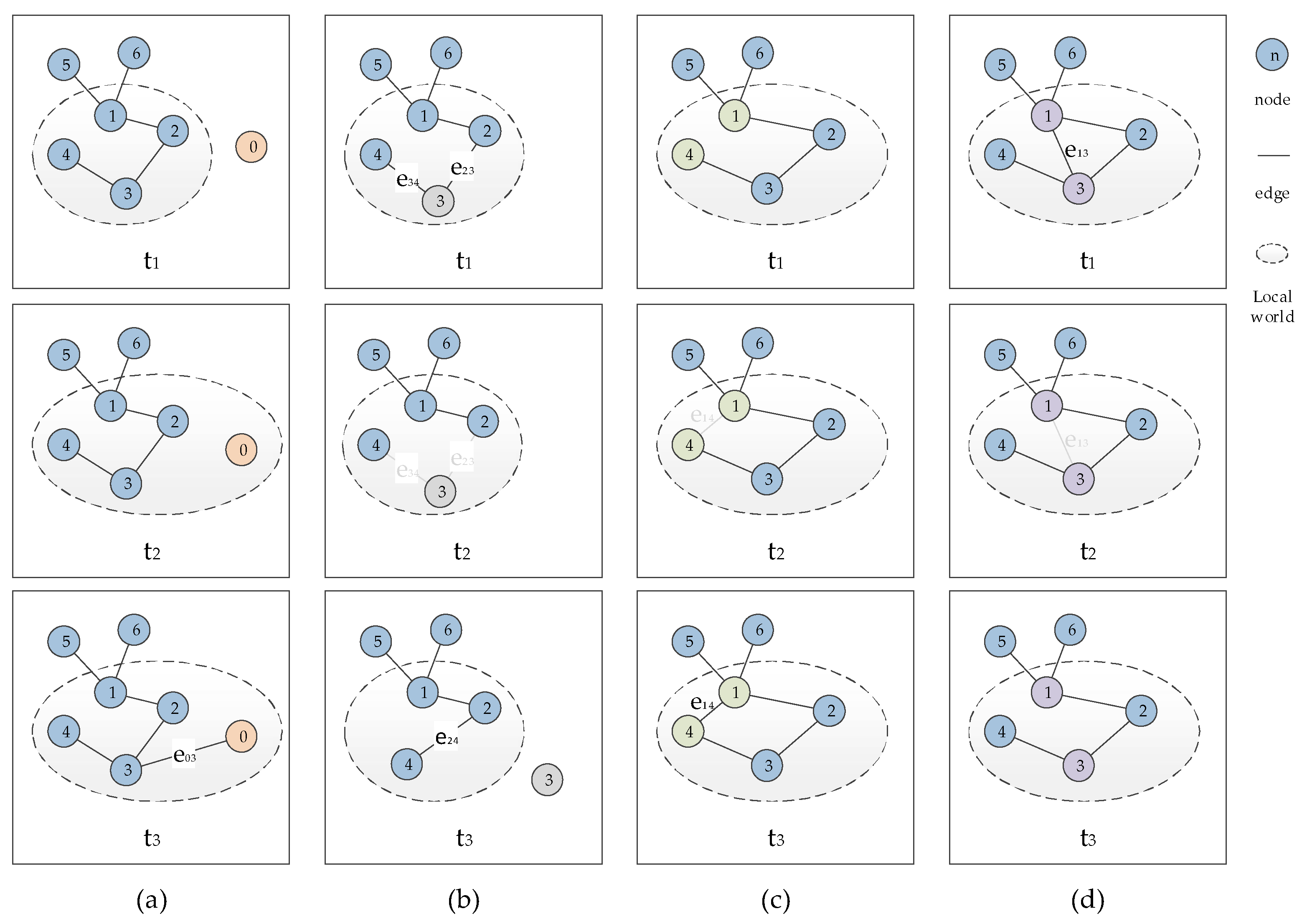
3.1. SIN Dynamic Evolution Rules

Existing network evolution models focus on the growth of nodes and edges to study evolutionary laws; however, the dynamic feature of SIN is more complex, and its evolution includes not only growth, but also deletions. Therefore, this section will provide different scenarios for the evolution of SIN, and through the establishment of topology evolution rules, it will combine the possible situations of the topology evolution of SIN one by one, thus guiding the development of the dynamic evolution model of the weighted local-world of SIN. For this reason, this part summarizes the following seven categories based on the situation in which the dynamic characteristics lead to changes in the topology, and establish their rules separately.

According to the topology evolution rules listed in Table 3 above, one by one detailed discussion will be pursued.

Table 3. SIN Topology Evolution Rules.

Number	Name	Number	Name
Rule 1	Node increase rule	Rule 5	Edge weight evolution rule
Rule 2	Edge increase rule	Rule 6	Node deletion rule
Rule 3	Local-World construction rule	Rule 7	Edge delete rule
Rule 4	Bidirectional selection rule

Rule 1: Node increase rule

The node increase rule mainly includes two situations. On the one hand, the number of nodes mapped to the topological domain increases when the equipment entities that make up the spatial information network increase, including the launch of satellites, the addition of aircrafts/balloons, and the addition of ground control stations. On the other hand, equipment entities such as satellites/aircrafts/balloons that do not move within the effective local-world are within a valid range at a certain moment, and are mapped to the topological domain, that is, the phenomenon of node increase.

Rule 2: Edge increase rule

The topology evolution analysis is applied when adding information/data interchange between equipment entities that make up SIN, including enabling connections between different equipment entities (e.g., enabling data/information exchange between certain equipment entities according to requirements, etc.), and enabling the connection between a ground control station and an equipment entity.

Rule 3: Local-world construction rule

When a new node is added, the node will be connected with the local network node, which involves the construction of the local-world. Combined with the structure of SIN, a newly added node $v_i$ is first connected in the corresponding layer domain before it is connected across the domain, and it also selects the neighbor node $v_j$ to connect. Symbol $\Omega$ represents the local-world, symbol $V_{Set}$ represents the set of nodes connected to the new node $v_i$, and symbol $V_{SubSet}$ represents the set of nodes connected to the same layer domain of the new node $v_i$.

$$\Omega =V_{Set}\cap V_{SubSet}$$

(7)

Rule 4: Bidirectional selection rule

When a new node is added, if two nodes want to establish a connection, then after a node $v_i$ sends a connection request to another node $v_j$ and waits for another node to identify, a valid connection is established between the two nodes. Therefore, it is necessary to establish a bidirectional preferred selection rule. Meanwhile, it is important to not only consider the connections within the local-world, but to also consider the connections outside the local-world.

In the local-world, a node $v_i$ is randomly selected as one side of the newly added edge, and the other endpoint performs a two-way preferential selection according to the probability $p_a$.

$$p_a={{\displaystyle \prod }}_{i,j\in local}\left(i\to j\right)=\frac{s_j}{{\sum }_{k\in local}{s}_k-s_i}$$

(8)

Outside the local-world, a node in the local-world is selected as the end of the new edge according to the probability of $p_b$.

$$p_b={{\displaystyle \prod }}_{i\in local}=\frac{s_i}{{\sum }_{k\in local}{s}_k}$$

(9)

Then, according to the probability of $p_c$, the other side of the new edge is selected outside the local-world, that is, the probability of selecting a node with a large intensity is larger.

$$p_c={{\displaystyle \prod }}_{j\in local-world}=\frac{s_j}{{\sum }_{k\in local-world}{s}_k}$$

(10)

In order to facilitate the later calculation, this paper only considers the circumstances of the two-way merit selection in the case of deletion of the internal edges of the local-world. Therefore, in the local-world, a node $v_i$ is randomly selected as the end of the edge to be eliminated, and the other end is chosen in the local-world according to the probability of $p_d$.

$$p_d=1-{{\displaystyle \prod }}_{j\in local}=1-\frac{s_j}{{\sum }_{k\in local}{s}_k}$$

(11)

Rule 5: Edge weight evolution rule

After adding edges, a weight ${\omega }_0$ is added to each newly added edge $e_i$, and for ease of calculation, it is assumed that the newly added edge will only partially cause the weights adjustment of the connection node $v_i$ and its neighbor node $v_j$. There is an evolutionary rule

$${\omega }_{ij}\to {\omega }_{ij}+\Delta {\omega }_{ij}$$

(12)

where, $\Delta {\omega }_{ij}={\alpha }_i\frac{{\omega }_{ij}}{s_i}$, and each time a new edge $e_i$ is introduced, additional traffic ${\alpha }_i$ will be brought to node $v_i$. The connected edges share a certain amount of traffic according to their own weight ${\omega }_{ij}$. So the strength of node $v_i$ is readjusted to:

$$s_i\to s_i+{\alpha }_i+{\omega }_0$$

(13)

where, the meaning of the symbol is the same as above.

Rule 6: Node deletion rule

When we delete the equipment entities, this rule applies to the topology evolution analysis, including actions such as the failure of satellites, failure of aircraft/balloon recycling, or cancellation or failure of the ground control station. Physical equipment such as satellites/aircraft/balloons has exceeded the scope of effective local information transmission (such as two-level areas), resulting in the failure of normal data/information exchange and the absence of new connections that can be re-enabled.

Rule 7: Edge deletion rule

The topology evolution analysis is applied when deleting information/data exchanges between equipment entities that make up a spatial information network, including disabling connections between different equipment entities (for example, if one equipment entity runs to another equipment entity data connected to it). When the effective range of the information exchange is out of range, the connection behavior between a ground control station and an equipment entity is deactivated, or some nodes delete more than one corresponding edge disconnection behavior.

3.2. SIN Dynamic Evolution Model

The most influential research on weighted network modeling is the weighted scale-free network model proposed by Barrat, Barthélemy, and Vespignani, known as the BBV model [31]. The model considers factors such as network structure and weights of nodes to study the dynamic evolution of the network. The BBV model has the characteristics of a simple structure and easy theoretical analysis, and as the model scale continues to increase, the degree, edge weights, and node weights of the BBV model network all exhibit scale-free characteristics. A large number of empirical studies have proved that most networks have edge weights, and network models that consider edge weights can more accurately reflect the structural characteristics of the network. Therefore, this paper comprehensively considers the edge-attributes of SIN and the phenomenon of the local-world. Based on this, it constructs the weighted local-world dynamic evolution model of SIN. Combined with the research content of the previous section, this section presents the concrete implementation algorithm and implementation flow of the weighted local-world dynamic evolution model of SIN.

3.2.1. Evolution Mechanism Analysis

In this paper, we mainly consider two factors. One is the local-world phenomenon, and the other is edge-weight. Therefore, we analyze the weighted local-world evolution mechanism and edge-weight evolution mechanism in this section.

(a) Local-world evolution mechanism

The local-world phenomenon of SIN has been discussed thoroughly in Section 2.3. As with most real networks, the priority connection mechanism for SIN also occurs within a local-world rather than a globally preferred connection. Therefore, each node has its own local-world. In order to visually display the local-world evolution mechanism, we present graphs from four perspectives, including node increase, node deletion, edge increase, and edge deletion, as shown below.

As shown in Figure 2, we use four perspectives to demonstrate the local-world evolution mechanism. We focus on three moments, including time $t_1$, $t_2$, and $t_3$. By comparing the similarities and differences in the topology structure at different moments, we can reflect its evolution mechanism. In the above process, we implement the priority connection mechanism and the selective deletion mechanism. This corresponds to the real network and has a stronger operability.

Figure 2. Local-world evolution mechanism: (a) Node increase mechanism; (b) Node deletion mechanism; (c) Edge increase mechanism; (d) Edge deletion mechanism.

(b) Edge-weight evolution mechanism

In Section 2.2.1, we have defined the multi-attribute node, that is, each node has multiple functions in SIN. Therefore, data and information are passed between nodes. If a node has multiple functions, it establishes connections with neighboring nodes. If two adjacent nodes establish more connections, the greater the weight between them. For intuitively displaying the edge-weight evolution mechanism, we present graphs, as shown below.

As shown in Figure 3, assume that the networks implement three functions at time $t_1$, as shown in Figure 3a–c, respectively. When we implement these three independent networks in an overall network topology, we can get Figure 3d. Compared with Figure 3a–c, we can find that the lines in Figure 3d that represent the edges are thicker, which is also a reflection of the edge-weight of the network. Therefore, the nodes that bear more functions will have a greater edge-weight with their neighboring nodes, which is also the core link of the edge-weight evolution.

Figure 3. Edge-weight evolution mechanism: (a) Network topology when implementing function 1 at time $t_1$; (b) Network topology when implementing function 2 at time $t_1$; (c) Network topology when implementing function 3 at time $t_1$; (d) Overall network topology at time $t_2$.

3.2.2. Evolution Model Construction Algorithm

• (1): Initial setting. At the beginning of the network, there are $m_0$ nodes and $e_0$ edges, and they form a fully coupled network in which weights $w_0$ are assigned to each edge.
• (2): Growth. Each time a new node $v_n$ is added and this node is connected to the previous $m$ nodes.
• (3): Local-world priority connection. Randomly select $M$ ($M\ge m)$ nodes from the existing nodes of the network as the newly joined node’s local-world. Newly added nodes according to the probability (${\prod }_{Local}\left(s_i\right)$) of preferential connection connect with $m$ nodes in the local-world, and the probability of strength selection is:

  $${\displaystyle {\displaystyle \prod }_{Local}}\left(s_i\right)={\displaystyle {\displaystyle \prod }_{i\in Local’}}\frac{s_i}{{\sum }_{j\in Local}{s}_j}$$

  (14)

  where, $\prod i\in Local\text{’}$ indicates the probability of randomly selecting nodes in existing nodes, and the choice of nodes is based on the priority of weight selection, that is, the probability that an old node $v_i$ is selected is:

  $${{\displaystyle \prod }}_{i\in Local’}=\frac{M}{N\left(t\right)}$$

  (15)

  where, $N\left(t\right)$ is the total number of nodes in the network at time $t$. When the time interval for joining the nodes is unchanged, there is $N\left(t\right)=N+t$. As shown above, this means that there is a greater probability that a node with a greater weight is selected. Obviously, at time $\left(m\le M\le N+t\right)$, and at each moment, the newly added node selects $m$ nodes from the local-world according to the preferential connection mechanism to establish a connection, and therefore, $m$ edges are newly added each time.
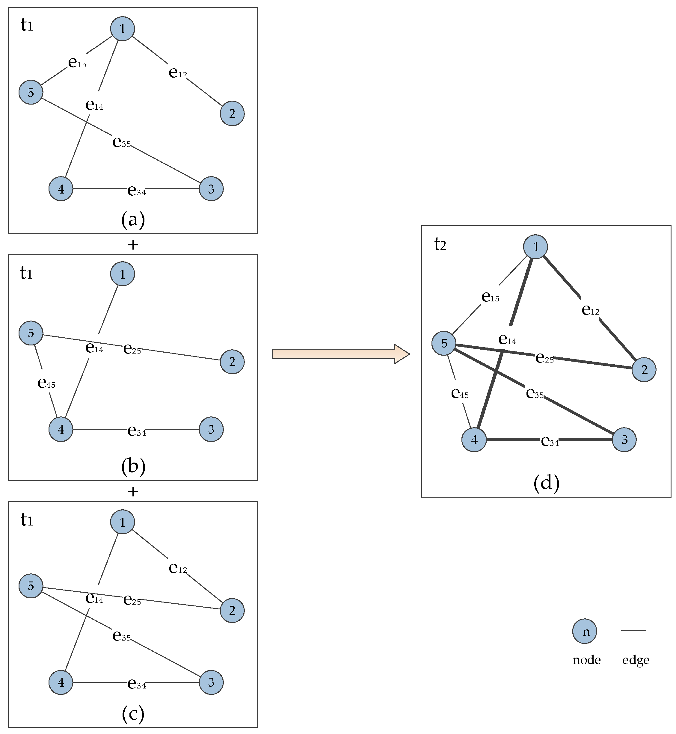
• (4): Dynamic evolution of edge weights. Each time the newly added edge $e_i$ is given a weight ${\omega }_0$. For the sake of simplicity, it is considered that the newly added edge only partially causes the weights of the edge of the connection node $v_i$ and its neighbor node $j\in \tau \left(i\right)$ to be readjusted, and the adjustment method is implemented according to the content of rule 4.

3.2.3. Evolution Model Implementation Process

Combining the inseparability of topology structure and evolution, we believe that the topology model of SIN is the initial moment of its dynamic evolution model, that is, the model with $t=t_0=0$. Therefore, based on the previous research contents, the implementation process of the weighted local-world dynamic evolution model of SIN is formulated, and the specific content is as follows.

• Step 1: At the initial time $t_0=0$, the initial topology model of SIN is generated, the initial time is a fully-coupled network with $n$ nodes and $e_0$ edges, and each edge is given an initial value $w_0$. The hierarchy is denoted by the symbol $H$($H\in \left[1,4\right]$).
• Step 2: At the time $t=t_0+\Delta t$, randomly select $M(M<n)$ nodes as a local-world from the generated SIN, and proceed with the following operation with a certain probability. Assume that the time $t$ obeys the exponential distributions of the parameter of $\beta$, and when the evolution time $t=t_n$, the evolution is complete.

  (a)

  Adding a new node $v_i$ to the local-world with a probability of $p_1$, and this node establishes a connection with the existing $m$ nodes in the local-world. The connecting nodes are preferably taken in accordance with the probabilistic Equation (8). The dynamic evolution of edge weights is the same as that of rule 4.

  (b)

  Adding $m_1$ as a new edge to the local-world with the probability of $p_2$, and in the local-world, one node is randomly selected as one end of the edge, and the other end is selected in the local-world by the content of rule 5.

  (c)

  Increasing the number of new edges $m_2$ inside the local-world and outside the local-world with a probability of $p_3$, and increasing the number of connections inside and outside the local-world. In the local-world, the node of the network is selected as the end of the edge by Equation (9), and the other end is selected outside the local domain by Equation (10).

  (d)

  Deleting $m_3$ links with a probability of $p_4$, randomly selecting one point as the edge of the edge in the local-world, and selecting the other using Equation (11) with rule 5 in the local-world.

  Among them, $p_1+p_2+p_3+p_4=1$, and $p_1,p_2,p_3,p_4>0$.

• Step 3: Repeating Step 2 until $t=t_n$, ending the evolution.

3.3. SIN Evolution Evaluation Indicators

In order to characterize the SIN structure and structure attributes, this paper achieves the quantitative analysis by four indicators, including node degree, node strength, edge weight, and correlation of strength and degree.

(a)

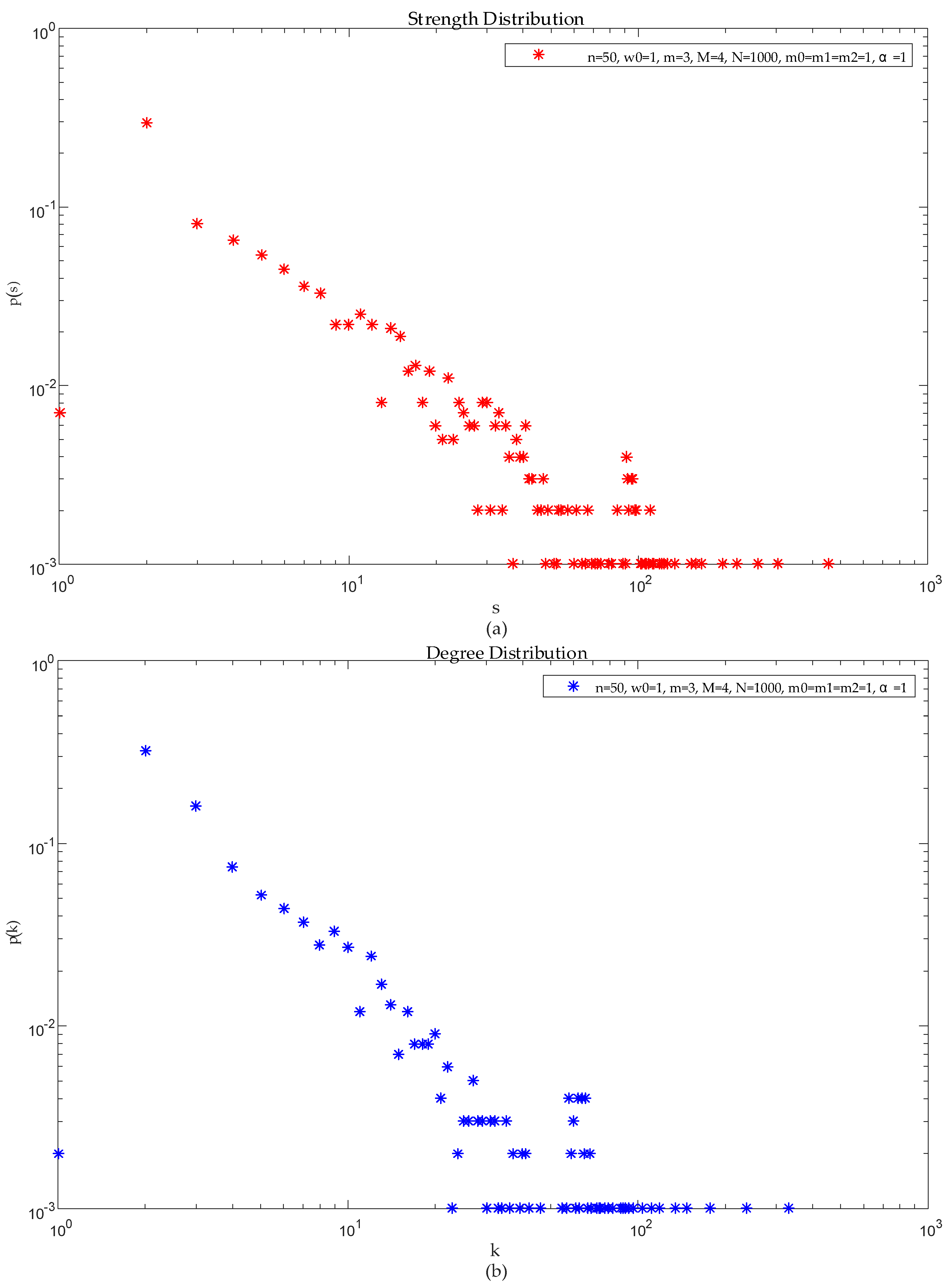
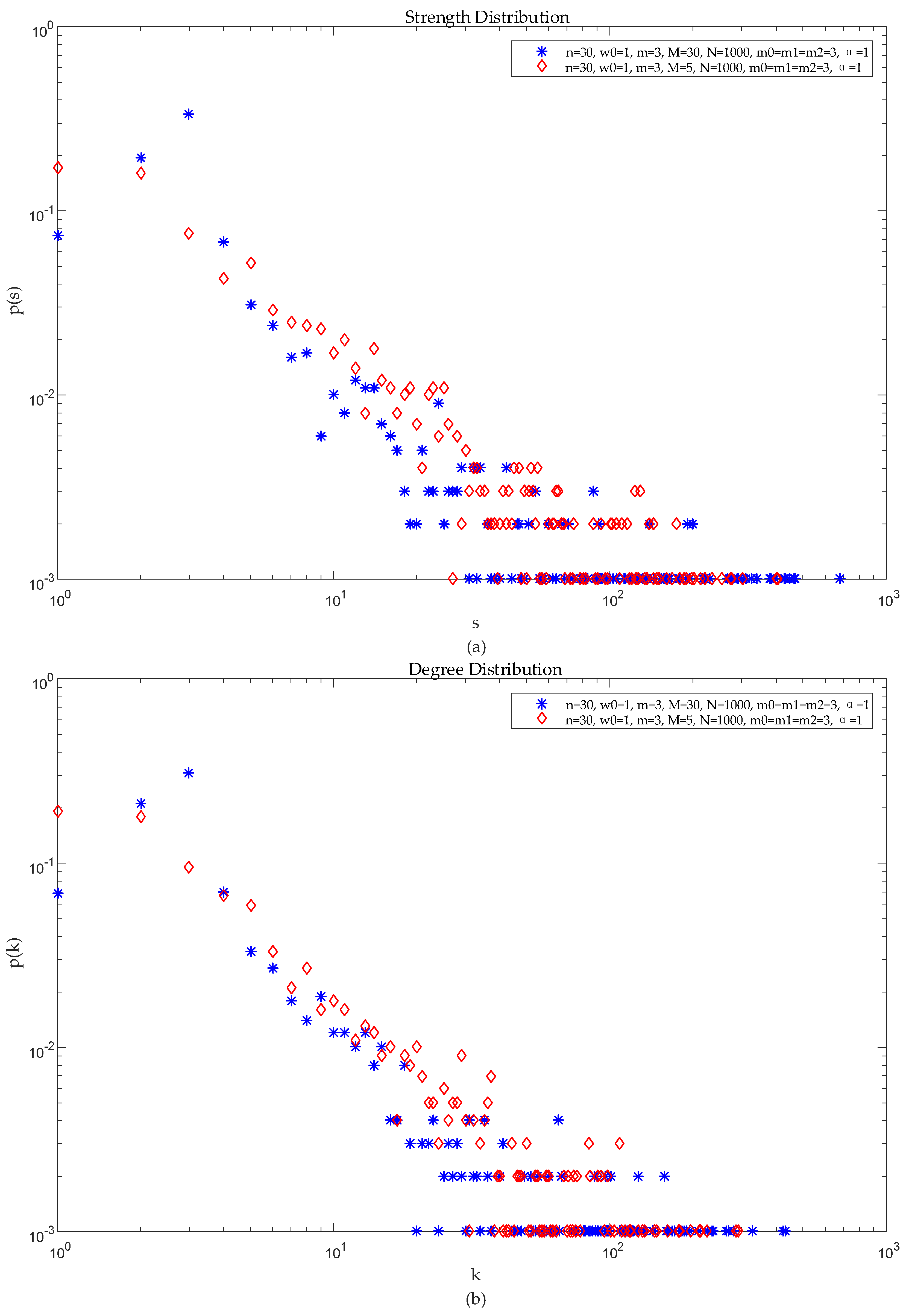
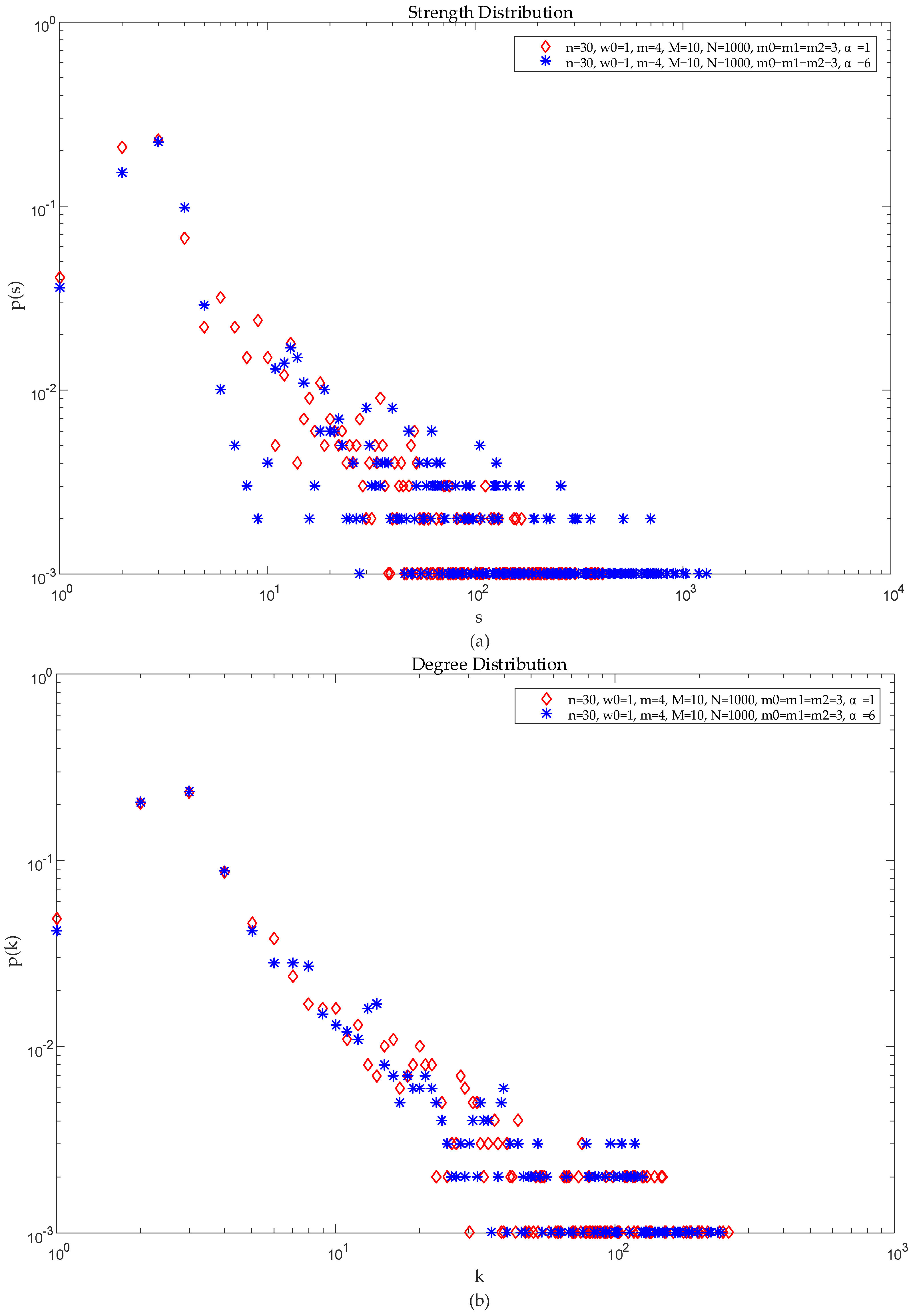
Node degree

Node degree is an important index used to describe the importance of nodes in weighted networks, and in SIN, the greater the degree of a core node, the more important it is in the entire network.

(b)

Node strength

Node strength is an important index to represent the weight of a node in a weighted network, and it is a concept introduced from an unlicensed network. In SIN, it is applied to indicate the importance of a certain node in the network.

(c)

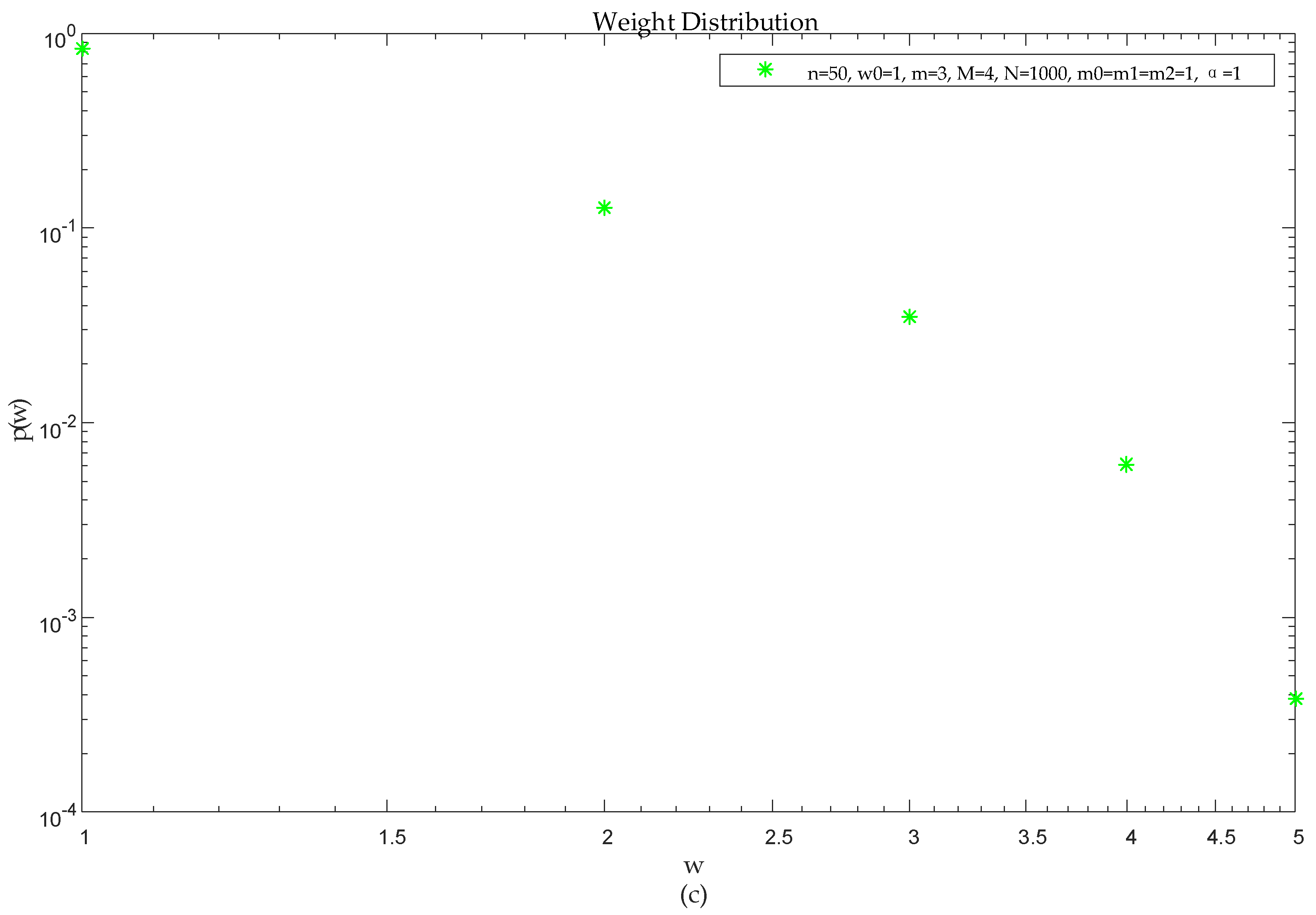
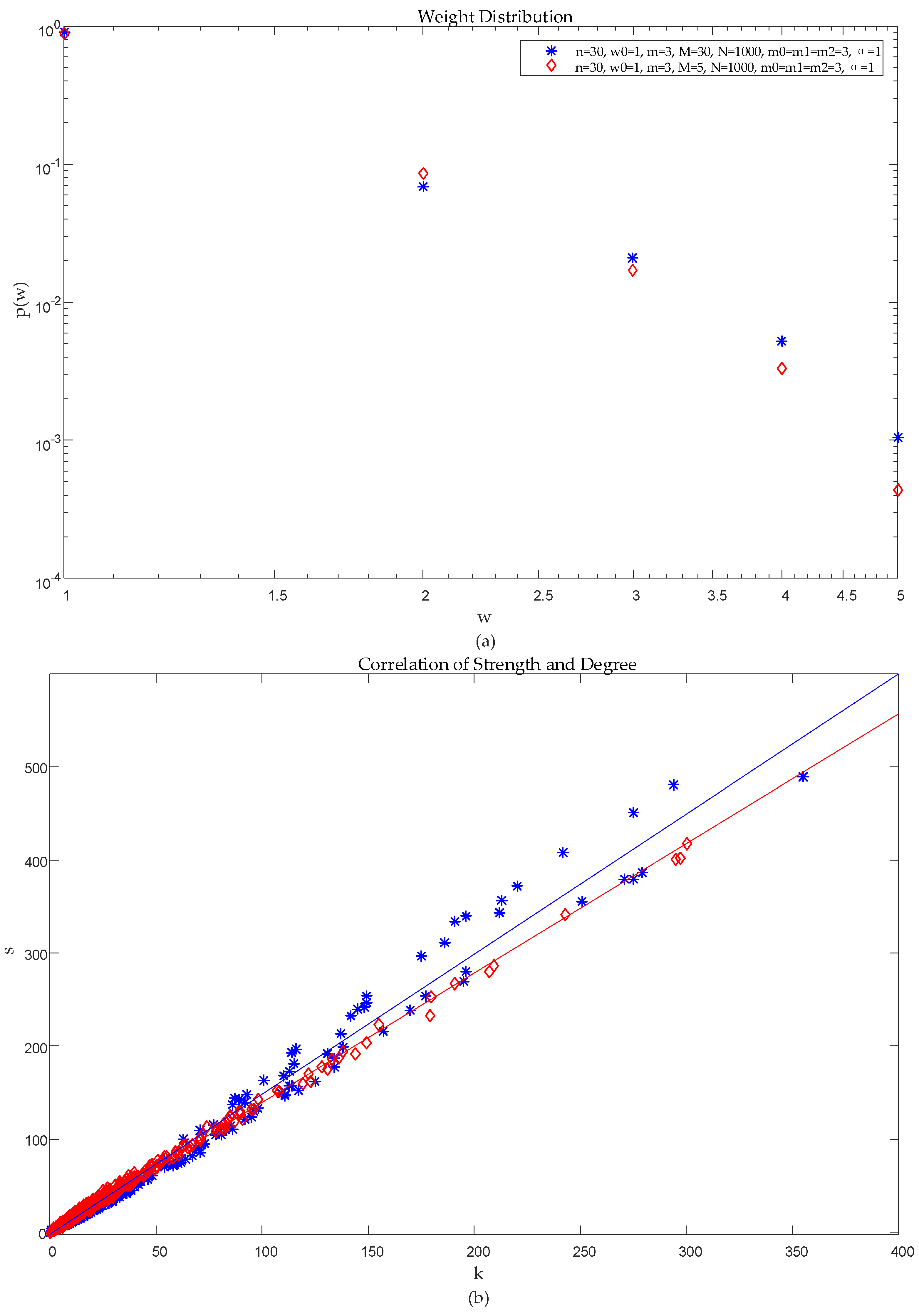
Edge weight

Edge weight is used to describe the closeness of two certain nodes, and the higher the degree of intimacy, the greater the weights; otherwise, the opposite is true. In SIN, because of the need to study the impact of its weight on the network evolution model, it is necessary to analyze its edge weight.

(d)

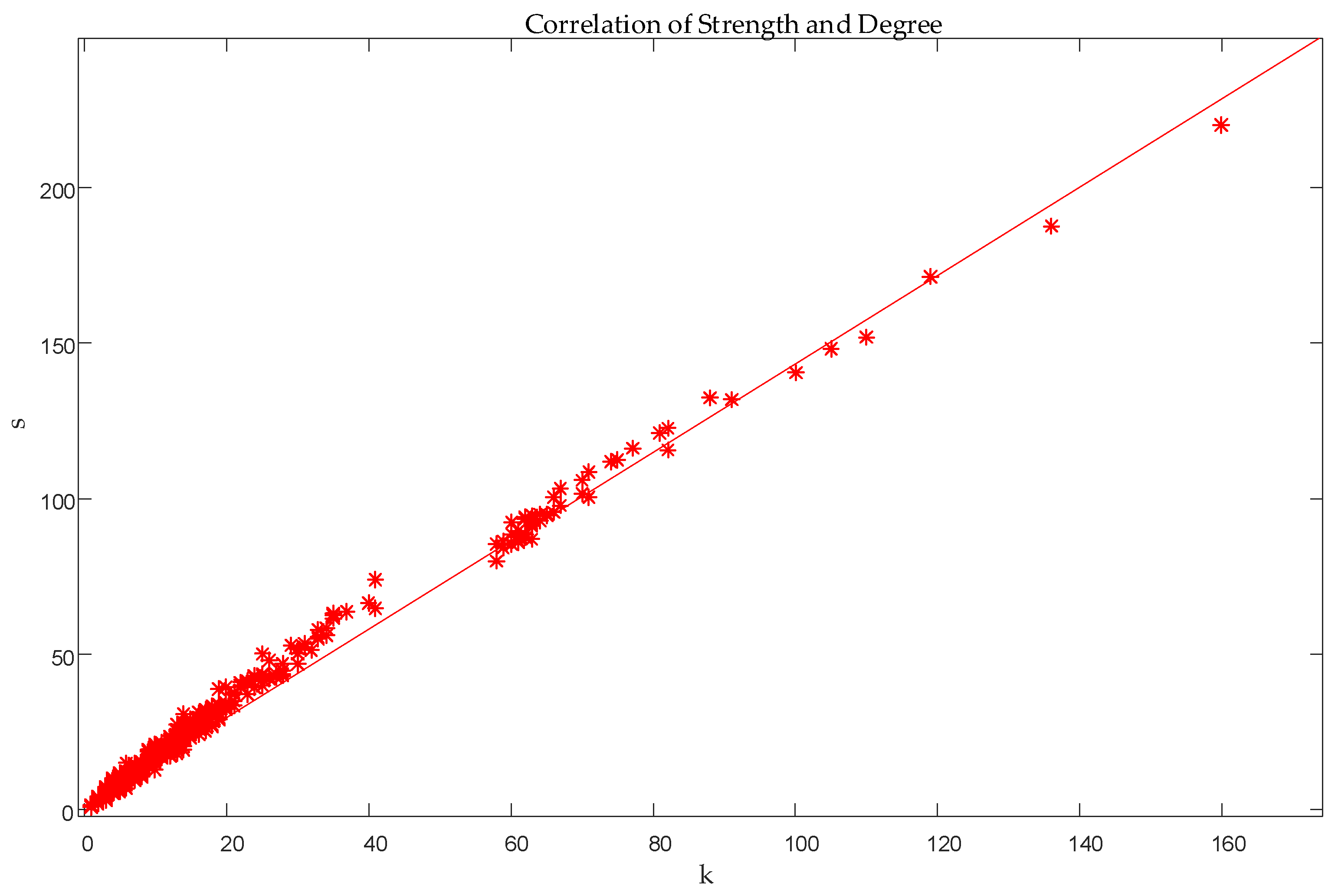
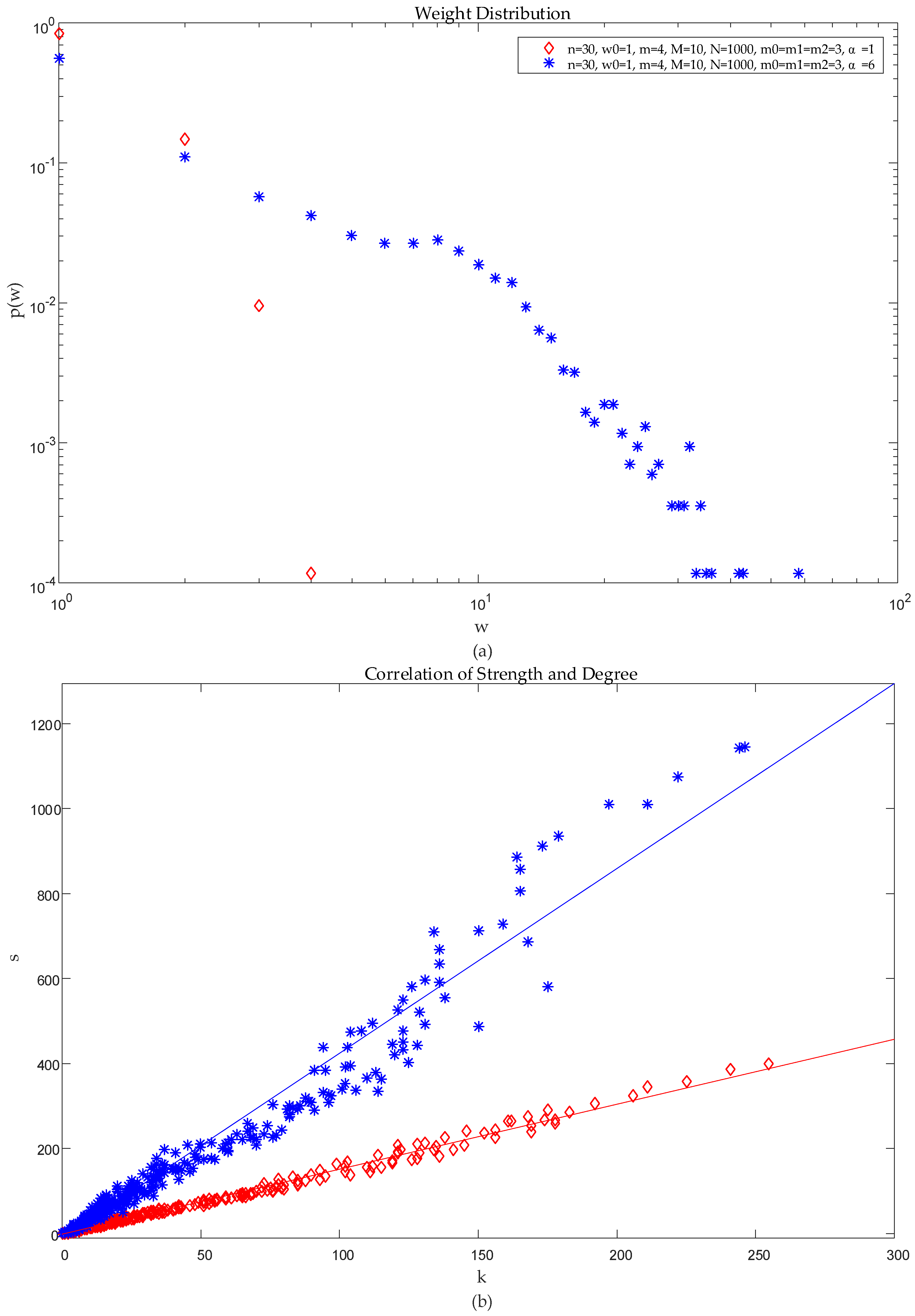
Correlation of strength and degree

Correlation of strength and degree is mainly used to respond to the best choice in SIN, and if a certain node is selected with a high probability, its node strength is positively correlated with the node degree; otherwise, the opposite is true.

4. Results

The purpose of this section is to analyze the validity and feasibility of the previously proposed model from both theory and simulation perspectives.

4.1. Theory Analysis

According to the related content of reference [32], using related knowledge of continuous medium theory, mean field theory, and algebraic theory, the distribution law of node strength in the constructed network model is analyzed, and the validity of the model is analyzed from a theoretical level.

Assumptions: The node strength $s_i$ is continuously changed, and the evolution time $t$ is also continuously changed. According to the implementation flow, the change rate of $s_i$ is deduced as follows.

According to the step in (a) in Section 3.2.3, the edge-weight caused by newly added nodes evolves to:

$$\begin{array}{cc}\hfill \frac{d{w}_{ij}\left(t\right)}{dt}& =m{p}_1{\displaystyle {\displaystyle \prod }_{local\left(v_i\right)}}\alpha \frac{w_{ij}}{s_i\left(t\right)}+m{p}_1{\displaystyle {\displaystyle \prod }_{local\left(v_j\right)}}\alpha \frac{w_{ij}}{s_j\left(t\right)}\hfill \\ & =m{p}_1\frac{M}{N\left(t\right)}\left(\frac{s_i\left(t\right)}{{{\displaystyle \sum }}_{k\in local}{s}_k\left(t\right)}\alpha \frac{w_{ij}\left(t\right)}{s_i\left(t\right)}+\frac{s_j\left(t\right)}{{{\displaystyle \sum }}_{k\in local}{s}_k\left(t\right)}\alpha \frac{w_{ij}\left(t\right)}{s_j\left(t\right)}\right)\hfill \\ & =2m{p}_1\alpha \frac{M}{N\left(t\right)}\frac{w_{ij}\left(t\right)}{{{\displaystyle \sum }}_{k\in local}{s}_k\left(t\right)}\hfill \end{array}$$

(16)

and the rate of change of $s_i$ is

$$\begin{array}{cc}\hfill {\left(\frac{d{s}_i}{dt}\right)}_1& =m{p}_1\frac{M}{N\left(t\right)}\frac{s_i}{{{\displaystyle \sum }}_{k\in local}{s}_k\left(t\right)}+\frac{d{w}_{ij}\left(t\right)}{dt}\hfill \\ & =m{p}_1\left(1+2\alpha \right)\frac{M}{N\left(t\right)}\frac{s_i\left(t\right)}{{{\displaystyle \sum }}_{k\in local}{s}_k\left(t\right)}\hfill \end{array}$$

(17)

According to the step in (b) in Section 3.2.3, and because the connection is bidirectional, the corresponding edge weights will evolve according to the following equation:

$$\frac{d{w}_{ij}\left(t\right)}{dt}=\frac{s_j\left(t\right)}{{\sum }_{k\in local}{s}_k\left(t\right)-s_i\left(t\right)}\frac{s_i\left(t\right)}{{\sum }_{k\in local}{s}_k\left(t\right)-s_j\left(t\right)}$$

(18)

and the rate of change of $s_i$ is

$$\begin{array}{cc}\hfill {\left(\frac{d{s}_i}{dt}\right)}_2& =m_1{p}_2\frac{M}{N\left(t\right)}\left[\frac{1}{M}+\left(1-\frac{1}{M}\right){\displaystyle {\displaystyle \sum }_{j\in local}}\frac{d{w}_{ij}\left(t\right)}{dt}\right]\hfill \\ & \approx m_1{p}_2\frac{M}{N\left(t\right)}\left[\frac{1}{M}+\left(1-\frac{1}{M}\right)\frac{s_i\left(t\right)}{{\sum }_{k\in local}{s}_k\left(t\right)-s_i\left(t\right)}\right]\hfill \\ & \approx m_1{p}_2\frac{M}{N\left(t\right)}\left[\frac{1}{M}+\left(1-\frac{1}{M}\right)\frac{s_i\left(t\right)}{{\sum }_{k\in local}{s}_k\left(t\right)}\right]\hfill \end{array}$$

(19)

According to the step in (c) in Section 3.2.3, the rate of change of $s_i$ is:

$${\left(\frac{d{s}_i}{dt}\right)}_3=m_2{p}_3\frac{M}{N\left(t\right)}\frac{s_i\left(t\right)}{{\sum }_{k\in local}{s}_k\left(t\right)}+m_2{p}_3\left(1-\frac{M}{N\left(t\right)}\right)\frac{s_i\left(t\right)}{{\sum }_{k\notin local}{s}_k\left(t\right)}$$

(20)

According to the step in (d) in Section 3.2.3, the rate of change of $s_i$ is:

$${\left(\frac{d{s}_i}{dt}\right)}_4=-m_3{p}_4\frac{M}{N\left(t\right)}\left[\frac{1}{M}+\left(1-\frac{1}{M}\right)\left(1-\frac{s_i\left(t\right)}{{\sum }_{k\in local}{s}_k\left(t\right)}\right)\right]$$

(21)

In the previous content, it has been assumed that the time $t$ obeys the exponential distribution of the parameter $\beta$ in the weighted local-world dynamic evolution model of SIN, that is, $p\left(x\right)=\beta e^{-\beta x}(x>0)$. Therefore, $p_1\beta t$ nodes are added to the network at time $t$, and $p_1{\int }_0^t\beta e^{-\beta x}\mathrm{d}x=p_1-p_1{e}^{-\beta x}\approx p_1\beta t$. Therefore, the total number of nodes in the network is:

$$N\left(t\right)\approx n+p_1\beta t$$

(22)

And the sum of node strength in the network is:

$$\begin{array}{cc}S\left(t\right)\hfill & \hfill =2e_0+2{\int }_0^t\left[m{p}_1\left(1+\alpha \right)++m_1{p}_2+m_2{p}_3-m_3{p}_4\right]p\left(x\right)\mathrm{d}x\\ & \approx 2e_0+2\left[m{p}_1\left(1+\alpha \right)++m_1{p}_2+m_2{p}_3-m_3{p}_4\right]\beta t\hfill \end{array}$$

(23)

The sum of node strength in the internal of the local-world is:

$${\displaystyle {\displaystyle \sum }_{k\in local}}{s}_k\left(t\right)=S\left(t\right)\frac{M}{N\left(t\right)}$$

(24)

The sum of node strength of in the external of the local-world is:

$${\displaystyle {\displaystyle \sum }_{k\notin local}}{s}_k\left(t\right)=S\left(t\right)\left(1-\frac{M}{N\left(t\right)}\right)$$

(25)

When time $t$ is large enough, $N\left(t\right)\approx p_1\beta t$ and $S\left(t\right)\approx 2\left[m{p}_1\left(1+\alpha \right)+m_1{p}_2+m_2{p}_3-m_3{p}_4\right]\beta t$. This results in the following relationship:

$$\begin{array}{c}\frac{d{s}_i}{dt}={\left(\frac{d{s}_i}{dt}\right)}_1+{\left(\frac{d{s}_i}{dt}\right)}_2+{\left(\frac{d{s}_i}{dt}\right)}_3+{\left(\frac{d{s}_i}{dt}\right)}_4\\ =\left[m{p}_1\left(1+2\alpha \right)+m_1{p}_2\left(1-\frac{1}{M}\right)+2m_2{p}_3+m_3{p}_4\left(1-\frac{1}{M}\right)\right]\frac{s_i}{S\left(t\right)}+\frac{m_1{p}_2-m_3{p}_{4}M}{N\left(t\right)}\\ =\frac{m{p}_1\left(1+2\alpha \right)+m_1{p}_2\left(1-\frac{1}{M}\right)+2m_2{p}_3+m_3{p}_4\left(1-\frac{1}{M}\right)}{2\left[m{p}_1\left(1+\alpha \right)+m_1{p}_2+m_2{p}_3-m_3{p}_4\right]\beta }\frac{s_i}{t}+\frac{m_1{p}_2-m_3{p}_{4}M}{p_1\beta t}\end{array}$$

(26)

and makes

$$a=\frac{m{p}_1\left(1+2\alpha \right)+m_1{p}_2\left(1-\frac{1}{M}\right)+2m_2{p}_3+m_3{p}_4\left(1-\frac{1}{M}\right)}{2\left[m{p}_1\left(1+\alpha \right)+m_1{p}_2+m_2{p}_3-m_3{p}_4\right]\beta },b=\frac{m_1{p}_2-m_3{p}_{4}M}{p_1\beta }$$

(27)

That is, $\frac{d{s}_i}{dt}=a\frac{s_i}{t}+\frac{b}{t}$, and when $a\ne 0$, the initial condition is $s_i\left(t_i\right)=m$, which is obtained by the theory of ordinary differential equations, as follows:

$$s_i\left(t_i\right)=-\frac{b}{a}+\left(m+\frac{b}{a}\right){\left(\frac{t}{t_i}\right)}^a$$

(28)

With further operations, the intensity distribution of node $v_i$ is:

$$p\left(s\right)=exp\left[-\beta t{\left(\frac{m+\frac{b}{a}}{s+\frac{b}{a}}\right)}^{\frac{1}{a}}\right]\frac{\beta t}{a}\frac{{\left(m+\frac{b}{a}\right)}^{\frac{1}{a}}}{{\left(s+\frac{b}{a}\right)}^{\frac{1}{a}+1}}$$

(29)

For Taylor’s expansion of the exponential function in Equation (29), because $\mathrm{s}$ can be seen as an infinite function of $t$, $s\gg t,s\gg m$.When $t$ is large enough, the intensity distribution of node $v_i$ is similar to:

$$p\left(s\right)\approx \frac{\beta t}{a}\frac{{\left(m+\frac{b}{a}\right)}^{\frac{1}{a}}}{{\left(s+\frac{b}{a}\right)}^{\frac{1}{a}+1}}$$

(30)

among them, the power law distribution index is

$${\gamma }_s=\frac{1}{a}+1=\frac{2\left[m{p}_1\left(1+\alpha \right)+m_1{p}_2+m_2{p}_3-m_3{p}_4\right]\beta }{m{p}_1\left(1+2\alpha \right)+m_1{p}_2\left(1-\frac{1}{M}\right)+2m_2{p}_3+m_3{p}_4\left(1-\frac{1}{M}\right)}+1$$

(31)

Analysis: In Equation (31), assign different values to each probability, and the corresponding models are different:

(a)

When $p_1=1,p_2=0,p_3=0,p_4=0,\beta =1$, and at this time, ${\gamma }_s=\frac{1}{a}+1=\frac{4\alpha +3}{2\alpha +1}$. At this point, $s_i\left(t\right)$ is the change rate of the node strength of the BBV model.

(b)

When $p_1=1,p_2=0,p_3=0,p_4=0,\beta =1,\alpha =0$, edge weights no longer change, and this network is non-weighted networks. At this time, $s_i=k_i$ for all nodes, and $s_i\left(t\right)$ is the change rate of the node degree of the BA model.

(c)

When the time $t$ is large enough, the node intensity distribution of the model is a power law distribution, and the distribution index is $\frac{1}{a}+1$. When $\frac{1}{2}\le a\le 1$, the node intensity distribution of the model obeys a power-law distribution with an exponent of two to three, and related to the values of parameters p₁, p₂, p₃, p₄, β, M, α, m. By adjusting the values of different parameters, the weighted local area dynamic evolution model proposed in this paper can be implemented.

4.2. Example Analysis

To verify the validity and feasibility of the proposed evolutionary model, and combined with the theoretical analysis of the model in Section 4.1 and the model evaluation indicators given in Section 3.3, this section presents example verification analysis of this model based on the MATLAB R2015b platform. Based on the initial generation of SIN, the changes in the properties of the network topology are analyzed by analyzing the different values of the parameters p₁, p₂, p₃, p₄, β, M, α, m.

Background: A space-based information network is a typical type of SIN. This paper uses a space-based information network as an example for verification. The initial number of nodes of the space-based information network is $n$, and when time t evolves, the final number of nodes is $N$.

Assumptions:$t$ obeys the exponential distribution with $\beta$, and $\beta =1$. The probability of four events in the model is $p_1=0.6,p_2=0.2,p_3=0.15,p_4=0.05$.

Situation 1: Given the initial conditions to generate the model of SIN, analyze the network characteristics of the network model at this moment.

Determining the initial value assumes that $n=50$, $w_0=1$, $M=4$, $m=3$, $m_1=m_2=m_3=1$, $\alpha =1$, and $N=1000$. The distribution of node degree, node strength, and edge weights is shown in Figure 4, and the distribution of correlation of strength and degree is shown in Figure 5 below.

Figure 4. Space information network characteristics analysis at the initial moment: (a) Distribution of node strength; (b) Distribution of node degree; (c) Distribution of edge weights.

Figure 5. Space information network characteristics analysis at the initial moment: Distribution of the correlation of strength and Degree.

As shown in Figure 4a–c, the corresponding strength distribution, degree distribution, and power distribution of the model all obey the power law distribution, and this is the same as the result of the theoretical analysis in the previous section. In Figure 5, network node strength $s$ has a strong correlation with node $k$. In this SIN model, there is a preferential connection mechanism for newly added nodes. That is, newly added equipment entities are more inclined to make matching connections with similarly functional and identical nodes, and this is the same as the result of the theoretical analysis in the previous section.

Situation 2: Other conditions are determined, changing the value of the local-world $M$, and analyzing its impact on the features of the network topology.

Determining the initial value assumes that $n=30,w_0=1,m=3,m_1=m_2=m_3=3,\alpha =1,N=1000$. Comparative analysis of the similarities and differences of the distribution of node degree, node strength, and correlation of strength and degree and edge weights by changing the value of local-world $M$ is shown in Figure 6 and Figure 7 below.

Figure 6. Analysis of the influence of local-world $M$ on network structure performance: (a) Distribution of node strength; (b) Distribution of node degree.

Figure 7. Analysis of the influence of local-world $M$ on network structure performance: (a) Distribution of edge weights; (b) Distribution of the correlation of strength and Degree.

As shown in Figure 6, keeping the other parameters unchanged, give the assignments $M=30$ and $M=5$ to observe the changes in the power law exponential distribution. From Figure 6a,b, it can be seen that in the case where the assignment of other parameters is determined, the larger the value of the local-world $M$ is, the more nodes there are with a stronger intensity.

From Figure 7a,b, we can see that the value of $M$ does not affect the effectiveness of the merit selection. It does not affect the trend and the distribution law of edge weights.

Situation 3: Other conditions are determined, where changing the new node increases the value of extra traffic $\mathsf{\alpha }$, and its impact on the network topology features is analyzed.

Determining the initial value assumes that $n=30,w_0=1,M=10,m=4,m_1=m_2=m_3=3,N=1000$. Comparative analysis of the similarities and differences of the distribution of node degree, node strength, and correlation of strength and degree and edge weights by changing the value of extra traffic load $\alpha$ is shown in Figure 8 and Figure 9.

Figure 8. Analysis of the influence of extra traffic load $\alpha$ on network structure performance: (a) Distribution of node strength. (b) Distribution of node degree.

Figure 9. Analysis of the influence of extra traffic load $\alpha$ on network structure performance: (a) Distribution of edge weights; (b) Distribution of the correlation of strength and Degree.

As shown in Figure 8, keeping the other parameters unchanged, give the assignments $\alpha =1$ and $\alpha =6$ to observe the changes in the power law exponential distribution. From Figure 8a,b, it can be seen that the magnitude of $\alpha$ has little effect on the strength of nodes and nodes in the case of other parameter assignments.

As shown in Figure 9, it can be seen from the Figure 9a that the larger the value of $\alpha$ is, the higher the degree of precision between the nodes is. From Figure 9b, it can be seen that although there is still a preferred choice of connection, the larger the value of $\alpha$ is, the greater the additional traffics burden brought about by the newly added node. The correlation value is in the correlation line and the larger the left and right fluctuations, the greater the instability of the network’s preferences.

To sum up, this section considers three different scenarios to verify the simulation test, and the example simulation results and theoretical analysis results coincide exactly, thus verifying the effectiveness and feasibility of the proposed model.

5. Discussion

This article focuses on the weight and local-world phenomenon. Therefore, the proposed model is evaluated experimentally using two parameters: local-world $M$ and extra traffic load $\alpha$. What needs to be said is that we also carried out the simulation analysis of weight $w_0$. However, the simulation results show a similar pattern with extra traffic load $\alpha$, so we do not show and analyze the related simulation results again.

In Section 4.2, for the sake of analysis and explanation, we set the assumptions that $t$ obeys the exponential distribution with $\beta$ $\left(\beta =1\right)$, and presume that the probability of four events in the model is $p_1=0.6,p_2=0.2,p_3=0.15,p_4=0.05$. Meanwhile, we focus on three situations, including an initial moment situation, local-world situation, and extra traffic load situation, and we achieve the quantitative analysis by four indicators including node degree, node strength, edge weight, and correlation of strength and degree. Simulation results show that the corresponding strength distribution, degree distribution, and power distribution of the model all obey the power law distribution and this is the same as the result of the theoretical analysis. According to the simulation results, the validity and feasibility of the evolution model are demonstrated to some extent. That is, the evolutionary model we built is correct and feasible.

6. Conclusions

The dynamic topology evolution of SIN is a new direction formed by the intersection of SIN and complex network theory. The heterogeneity and complexity of SIN have brought challenges to the analysis of their topology structure and dynamic evolution. This paper addresses the demands of topological evolution modeling for SIN, and studies the weighted local-world dynamic evolution model. The simulation results are consistent with the theoretical results, which also validates the validity and feasibility of the model proposed. The method of this paper avoids the complexity of SIN and can carry out evolutionary analysis on its more active part, which reduces the complexity of research and reduces the unnecessary workload.

Of course, SIN is a complex and huge system, and several simulation experiments above are incomplete. In the future work, on the existing basis, we should further improve the evolution rules, enrich the evaluation indicators, and optimize the local-world selection method. Meanwhile, we can carry out the simulation verification in combination with the different situations. Beyond that, we also need to expand and enrich its evaluation indexes, such as the clustering coefficient, average path length, and so on. We believe that comprehensive consideration of these indicators can better verify the validity and feasibility of this model.

References

- Zhou, J.G. Research on Key Technology of Spatial Information Network Based on DTN; Wuhan University: Wuhan, China, 2013; pp. 1–5. [Google Scholar]
- Li, D.R.; Shen, X.; Gong, J.Y.; Zhang, J.; Lu, J. On construction of China’s space information network. J. Wuhan Univ. Inf. Sci. Ed. 2015, 40, 711–715. [Google Scholar]
- Yu, Q.Y.; Meng, W.X.; Yang, M.C.; Zheng, L.M.; Zhang, Z.Z. Virtual multi-beamforming for distributed satellite clusters in space information networks. IEEE Wirel. Commun. 2016, 23, 95–101. [Google Scholar] [CrossRef]
- Yu, S.B.; Wu, L.D.; Zhang, X.T.; Li, C.; Ma, H.J. Survey of multi-feature visualization for space information network. J. CAEIT 2018, 13, 201–208. [Google Scholar]
- Baidu, Baike. Topology. Available online: https://baike.baidu.com/item/Topology/573536?fr=aladdin.html (accessed on 6 November 2014).
- Carstens, C.J. Topology of complex networks: Models and analysis. Bull. Aust. Math. Soc. 2017, 95, 347–349. [Google Scholar] [CrossRef]
- Khan, I.; Belqasmi, F.; Glitho, R.; Crespi, N.; Morrow, M.; Polakos, P. Wireless sensor network virtualization: A survey. IEEE Commun. Surv. Tutor. 2017, 18, 553–576. [Google Scholar] [CrossRef]
- Faloutsos, M.; Karagiannis, T.; Moon, S. Online Social Networks. Comput Commun. 2016, 73, 163–166. [Google Scholar] [CrossRef]
- Li, X.; Chen, G. A local-world evolving network model. Phys. A Stat. Mech. Appl. 2003, 328, 274–286. [Google Scholar] [CrossRef]
- Zhu, H.; Luo, H.; Peng, H.; Li, L.; Luo, Q. Complex networks-based energy-efficient evolution model for wireless sensor networks. Chaos Sol. Fractal 2009, 41, 1828–1835. [Google Scholar] [CrossRef]
- Wang, H.F. Research on the Evolution Model of Wireless Sensor Network and Its Anti-Destructiveness; Xi’an Electronic Science and Technology University: Xi’an, China, 2014; pp. 15–22. [Google Scholar]
- Fu, X.W.; Li, W.F. Evolutionary model of heterogeneous clustering wireless sensor networks based on local world theory. J. Commun. 2015, 36, 64–72. [Google Scholar]
- Leberknight, C.; Inaltekin, H.; Chiang, M.; Poor, H.V. The Evolution of Online Social Networks: A tutorial survey. IEEE Signal Process. Mag. 2012, 29, 41–52. [Google Scholar] [CrossRef]
- Wang, R.L.; Cai, G.Y.; Lin, H. A new online social network evolving model. Comput. Eng. 2012, 38, 72–74. [Google Scholar]
- He, J.; Guo, J.L.; Xu, X.J. Research on micro-blog relationship network model. Comput. Eng. 2013, 39, 105–108. [Google Scholar]
- Zhang, X.; Chen, C.; Han, D.D. An evolution model of online social networks based on “sina micro-blog”. J. Shanghai Normal Univ. Nat. Sci. Ed. 2016, 45, 320–328. [Google Scholar]
- Zhang, B.; Li, Y.T. A review of the evolution model of scientific knowledge network. J. China Libr. Sci. 2016, 42, 85–101. [Google Scholar]
- Sun, Y.; Jiao, L.; Deng, X. Dynamic network structured immune particle swarm optimisation with small-world topology. Int. J. Bio-Inspired Comput. 2017, 9, 93–105. [Google Scholar]
- Sun, X.L. The Structure of Cooperative Network and Its Evolution and Prediction Research; Dalian University of Technology: Dalian, China, 2014; pp. 5–12. [Google Scholar]
- Tian, Z.H. Research on the Evolution Mechanism of Electronic Commerce Market Network Based on Self-Organization Theory; Beijing Jiaotong University: Beijing, China, 2016; pp. 41–47. [Google Scholar]
- Wang, Y.M.; Pan, C.S.; Chen, N.B.; Zhang, D.P. Evolution model of weighted command and control network based on local world. J. Syst. Eng. Electron. 2017, 39, 1596–1603. [Google Scholar]
- Zhang, Q.; Li, J.H.; Shen, D.; Zhao, J.W. Dynamic evolution model of operational network based on complex network theory. J. Harbin Inst. Technol. 2015, 47, 106–112. [Google Scholar]
- Oubbati, O.S.; Lakas, A.; Zhou, F.; Güneş, M.; Yagoubi, M.B. A survey on position-based routing protocols for Flying Ad hoc Networks (FANETs). Veh. Commun. 2017, 10, 29–56. [Google Scholar] [CrossRef]
- Gupta, L.; Jain, R.; Vaszkun, G. Survey of Important Issues in UAV Communication Networks. IEEE Commun. Surv. Tutor. 2016, 18, 1123–1152. [Google Scholar] [CrossRef]
- Bekmezci, I.; Sahingoz, O.K.; Temel, Ş. Flying ad-hoc networks (FANETs): A survey. Ad Hoc Netw. 2013, 11, 1254–1270. [Google Scholar] [CrossRef]
- Wu, B.; Yin, H.X.; Liu, A.L.; Liu, C.; Xing, F. Investigation and system implementation of flexible bandwidth switching for a software-defined space information network. IEEE Photonics J. 2017, 9, 1–14. [Google Scholar] [CrossRef]
- Yu, Q.; Wang, J.C.; Bai, L. Architecture and critical technologies of space information networks. J. Commun. Inf. Netw. 2016, 1, 1–9. [Google Scholar] [CrossRef]
- Yu, S.B.; Wu, L.D.; Zhang, X.T. Data as a center: An architecture modeling of space information network. J. Commun. 2018, 38, 165–170. [Google Scholar]
- Qin, S.; Dai, G.Z. A new local-world evolving network model. Chin. Phys. B 2009, 18, 383–390. [Google Scholar]
- Dai, M.Z.; Zhang, L.L. Topology properties of a weighted multi-local-world evolving network. Can. J. Phys. 2015, 93, 353–360. [Google Scholar] [CrossRef]
- Barrat, A.; Barthélemy, M.; Vespignan, A. Weghted evolving netwarks: Coupling topology and weighted dynamics. Phys. Rev. Lett. 2004, 92, 228701. [Google Scholar] [CrossRef] [PubMed]
- Mu, X.Q.; He, H.; Wang, J.H. Research on the model of the financial network evolution based on the weighted local-world. J. Syst. Sci. Math. Sci. 2017, 37, 1272–1286. [Google Scholar]