Ternary LWE Key Search: A New Frontier for Quantum Combinatorial Attacks

Abstract

The Learning with Errors (LWE) problem, particularly its efficient ternary variant where secrets and errors are small, is a fundamental building block for numerous post-quantum cryptographic schemes. Combinatorial attacks provide a potent approach to cryptanalyzing ternary LWE. While classical attacks have achieved complexities close to their asymptotic ${\mathcal{S}}^{0.25}$ bound for a search space of size $\mathcal{S}$, their quantum counterparts have faced a significant gap: the attack by van Hoof et al. (vHKM) only reached a concrete complexity of ${\mathcal{S}}^{0.251}$, far from its asymptotic promise of ${\mathcal{S}}^{0.193}$. This work introduces an efficient quantum combinatorial attack that substantially narrows this gap. We present a quantum walk adaptation of the locality-sensitive hashing algorithm by Kirshanova and May, which fundamentally removes the need for guessing error coordinates—the primary source of inefficiency in the vHKM approach. This crucial improvement allows our attack to achieve a concrete complexity of approximately ${\mathcal{S}}^{0.225}$, markedly improving over prior quantum combinatorial methods. For concrete parameters of major schemes including NTRU, BLISS, and GLP, our method demonstrates substantial runtime improvements over the vHKM attack, achieving speedup factors ranging from $2^{16}$ to $2^{60}$ across different parameter sets and establishing the new state-of-the-art for quantum combinatorial attacks. As a second contribution, we address the challenge of polynomial quantum memory constraints. We develop a hybrid approach combining the Kirshanova–May framework with a quantum claw-finding technique, requiring only $\mathcal{O}\left(n\right)$ qubits while utilizing exponential classical memory. This work provides the first comprehensive concrete security analysis of real-world LWE-based schemes under such practical quantum resource constraints, offering crucial insights for post-quantum security assessments. Our results reveal a nuanced landscape where our combinatorial attacks are superior for small-weight parameters, while lattice-based attacks maintain an advantage for others.

1. Introduction

The Learning with Errors (LWE) problem [1] has become a cornerstone of post-quantum cryptography, serving as the security foundation for numerous cryptographic constructions [2,3,4]. In its standard form, LWE tries to find a secret vector $s\in {\mathbb{Z}}_q^n$ given $(A,b)\in {\mathbb{Z}}_q^{m\times n}\times {\mathbb{Z}}_q^m$, where A is a random matrix and $b=As+emodq$ for some small error vector e. The hardness of LWE is supported by worst-case lattice reduction proofs [5], making it a robust basis for cryptographic constructions.

A particularly efficient variant is ternary LWE, where the entries of s and e are restricted to $\{-1,0,1\}$. This variant is employed in several practical schemes, including NTRU-based cryptosystems [6,7,8] and signature protocols such as BLISS [9] and GLP [10]. While the small domain of the secret and error does not fundamentally break LWE’s security, it does enable more efficient combinatorial attacks that exploit the sparsity and structure of the secrets.

Combinatorial attacks offer a distinct approach to cryptanalyzing LWE with small secrets, beginning with early Meet-in-the-Middle (MitM) attacks on NTRU by Odlyzko [11] and Howgrave-Graham [12]. A significant advancement came from May [13], who adapted the representation technique from subset-sum attacks [14,15,16] to reduce MitM complexity from ${\mathcal{S}}^{0.5}$ to approximately ${\mathcal{S}}^{0.25}$ for a search space of size $\mathcal{S}$. However, this improvement required guessing sub-linear error coordinates, which, while asymptotically negligible, raised concrete complexities to ${\mathcal{S}}^{0.3}$ for practical NTRU, BLISS, and GLP parameters. This limitation was later addressed by Kirshanova and May [17] through an Odlyzko-based locality-sensitive hashing (LSH) technique that eliminated error guessing, finally achieving complexities near the asymptotic ${\mathcal{S}}^{0.25}$ bound.

In the quantum setting, van Hoof et al. [18] investigated quantum speedups for May’s algorithm. Their asymptotic analysis demonstrates that the approach achieves a time complexity close to the ${\mathcal{S}}^{0.193}$ bound; however, for concrete instantiations, the method only reaches a ${\mathcal{S}}^{0.251}$ bound. Despite employing quantum search to accelerate the guessing phase, their quantum approach inherits the same fundamental limitation: for concrete cryptographic parameters, the realized complexity substantially deviates from the asymptotic bound, failing to bridge the gap between theoretical and practical performance.

1.1. Our Contribution

This work introduces a quantum adaptation of the LSH-based algorithm by Kirshanova and May [17] for solving ternary LWE. We reformulate the key recovery problem within a graph search framework. By implementing an optimized quantum walk over this graph, we eliminate the need for guessing the error coordinates—a fundamental limitation inherent to the quantum approach of van Hoof et al. [18]. As a result, our method substantially narrows the gap between asymptotic and concrete complexity, achieving a concrete bound of approximately $S^{0.225}$ compared to the $S^{0.251}$ bound of vHKM. For concrete parameters of major schemes such as NTRU, BLISS, and GLP, our method demonstrates speedup factors ranging from $2^{16}$ to $2^{60}$ over the vHKM [18] attack.

Our algorithm establishes the state of the art for quantum combinatorial attacks on ternary LWE. A comparison with quantum sieving algorithm shows a split in dominance: our method is superior for small-weight parameters, while lattice-based attacks maintain the lead for most others.

Current LWE parameter selection relies heavily on lattice reduction heuristics (e.g., Gaussian Heuristic and Geometric Series Assumption) and diverse BKZ runtime models, potentially underestimating security. In contrast, our combinatorial approach builds on heuristic principles derived from subset-sum or knapsack problems, which possess a stronger theoretical foundation. For knapsack-type distributions, it can be rigorously proven that pathological instances form only an exponentially small fraction, enabling the construction of provable probabilistic algorithms that avoid heuristics entirely. This theoretical robustness, combined with experimental validation in prior work [15], provides runtime predictions with significantly enhanced precision compared to lattice reduction heuristics that depend on unproven assumptions.

Our second contribution focuses on LWE key recovery under polynomial quantum memory constraints. While previous quantum-walk-based approaches achieve optimal time complexity among combinatorial methods, they require exponential qubit resources and rely on the strong Quantum Random Access Quantum Memory (QRAQM) model.

Building on recent work by Benedikt [19], who applied the quantum claw-finding algorithm of Chailloux et al. [20] to ternary LWE problems, we adopt a more practical approach that combines the Kirshanova–May framework [17] with this claw-finding technique. This hybrid strategy operates efficiently with only $\mathcal{O}\left(n\right)$ qubits under the Quantum Random Access Classical Memory (QRACM) model.

While Benedikt [19] provided valuable asymptotic analysis, their work left open the question of concrete security estimates for practical cryptographic parameter sets. Our work specifically addresses this gap by performing the first comprehensive concrete security analysis of real-world LWE-based schemes under polynomial-qubit constraints, providing crucial insights for post-quantum security assessments.

Furthermore, we provide the time–classical memory trade-offs for concrete schemes and explicitly compare our approach with the vHKM [18] method under strict polynomial classical memory constraints. Notably, across all evaluated schemes, our algorithm consistently achieves lower time complexity than vHKM under the same polynomial memory bound, further establishing its practical relevance in constrained settings.

1.2. Organization

The rest of this paper is organized as follows. In Section 2, we provide the necessary background, including the definition of the Ternary LWE, an introduction to Generalized Odlyzko’s Locality-Sensitive Hashing, and a review of the quantum primitives used in this work: amplitude amplification and quantum walks. Section 3 reviews the classical LSH-based MitM attack on ternary LWE by Kirshanova and May, which serves as the foundation for our quantum algorithms. In Section 4, we present our main contribution. We reformulate the ternary LWE key search problem as a graph search problem and introduce our novel quantum algorithm that combines the Kirshanova–May framework with a quantum walk. We provide a detailed description of the algorithm and a comprehensive concrete security analysis for major cryptographic schemes. Section 5 addresses the scenario of polynomial quantum memory constraints. We present a second algorithm that hybridizes the Kirshanova–May framework with a quantum claw-finding technique, requiring only a polynomial number of qubits. The concrete security of real-world schemes under this new algorithm is thoroughly analyzed. Finally, we conclude the paper in Section 6 with a summary of our findings.

2. Preliminaries

2.1. Notational Conventions

We adopt the following notation throughout this paper:

• Let ${\mathbb{Z}}_q$ represent the quotient ring of integers modulo $q\ge 2$.
• Vector quantities are denoted using lowercase letters (e.g., x, y), while matrices use uppercase letters (e.g., A, B).
• For any vector x, its ${\ell }_{\infty }$-norm is defined as ${\parallel x\parallel }_{\infty }={max}_i\left|x_i\right|$.
• The cardinality of a set S is denoted by $\left|S\right|$.
• For positive integers n and ${\left\{n_i\right\}}_{i\le k}$ summing to n, the multinomial coefficient is given by the product

  $$\left({\displaystyle \genfrac{}{}{0pt}{}{n}{n_1,\dots ,n_{k-1},n_k}}\right)=\left({\displaystyle \genfrac{}{}{0pt}{}{n}{n_1}}\right)\left({\displaystyle \genfrac{}{}{0pt}{}{n-n_1}{n_2}}\right)\dots \left({\displaystyle \genfrac{}{}{0pt}{}{n-{\sum }_{i=1}^{k-1}{n}_i}{n_k}}\right).$$

  (1)
  A compact notation $\left({\displaystyle \genfrac{}{}{0pt}{}{n}{n_1,\dots ,n_{k-1},·}}\right)$ is commonly used, where the dot signifies the remaining value $n_k=n-{\sum }_{i=1}^{k-1}{n}_i$.

2.2. Ternary LWE Secret Key

We focus on LWE instances where both the secret and error vectors are ternary and matrix A is square. This specific case captures numerous practical implementations in lattice-based cryptography.

Definition 1

(Ternary LWE Secret Key). Let $(A,b)\in {\mathbb{Z}}_q^{m\times n}\times {\mathbb{Z}}_q^m$ be an LWE public key satisfying $As=b+emodq$. The pair $(s,e)$ is called a ternary LWE secret key if both s and e belong to the set ${\mathcal{T}}^n={\{-1,0,1\}}^n$, i.e., ${\parallel s\parallel }_{\infty }={\parallel e\parallel }_{\infty }=1$.

The ternary constraint ensures cryptographic efficiency while maintaining security guarantees. For a randomly chosen A, the correct solution s is uniquely identifiable with high probability through the condition that $As-b$ also falls within ${\mathcal{T}}^n$.

Practical implementations often impose additional structural constraints by fixing the number of non-zero entries in ternary vectors, leading to optimized security parameters and implementation characteristics.

Definition 2

(Weight). Let $s=(s_1,\dots ,s_n)\in {\mathbb{F}}_q^n$. The weight w of s is defined as its Hamming weight $w:={\sum }_{s_i\ne 0}1$. For ternary vectors with balanced non-zero coefficients, we define the specialized set:

$${\mathcal{T}}^n(w/2)=\left\{s\in {\mathcal{T}}^n\mid s\mathit{has}\mathit{exactly}w/21-\mathit{entries}\mathit{and}w/2(-1)-\mathit{entries}\right\}.$$

(2)

Rounding considerations are handled appropriately in concrete parameterizations. Weight restrictions naturally emerge in the context of NTRU-type cryptosystems, where optimal values typically reside in the interval $\omega \in [\frac{1}{3},\frac{2}{3}]$. The specific choice $\omega =\frac{3}{8}$ appears in several standardized parameter sets, representing a careful equilibrium between security and performance requirements.

2.3. Generalized Odlyzko’s Locality-Sensitive Hashing

A key technique in combinatorial attacks on ternary LWE is the use of LSH to efficiently identify pairs of vectors that are close in the ${\ell }_{\infty }$-norm. Odlyzko’s original LSH function [11] partitions ${\mathbb{Z}}_q$ into two halves and assigns binary labels, but it requires special handling of border values.

Kirshanova and May [17] generalized this approach to avoid explicit border checks and to enable more flexible bucketing. Their LSH family is defined as follows. For a bucket size parameter $B\in \{1,\dots ,q\}$ and a random shift vector $u\in {\mathbb{Z}}_q^n$, the hash function $h_{u,B}:{\mathbb{Z}}_q^n\to {\left[0,\lceil q/B\rceil -1\right]}^n$ is given by

$$h_{u,B}\left(x\right)=\left(⌊{\displaystyle \frac{x_1+u_1}{B}}⌋,\dots ,⌊{\displaystyle \frac{x_n+u_n}{B}}⌋\right).$$

(3)

This function maps each coordinate of x to a bucket index after a random cyclic shift. The probability that two vectors $x,y$ with ${\parallel x-y\parallel }_{\infty }=1$ collide under a random $h_{u,B}$ is ${(1-1/B)}^n$.

Algorithm 1 solves the close pairs problem in the ${\ell }_{\infty }$-norm: given two lists $L_1,L_2\subset {\mathbb{Z}}_q^n$, find a $(1-o(1\left)\right)$-fraction of all pairs $(x,y)\in L_1\times L_2$ such that ${\parallel x-y\parallel }_{\infty }=1$.

Example 1.

We illustrate Algorithm 1 with $n=4$, $q=7$, and lists:

$$\begin{array}{cc}\hfill L_1& =\left\{\right(1,0,2,3),(0,1,1,1),(2,3,0,1\left)\right\},\hfill \\ \hfill L_2& =\left\{\right(1,1,2,2),(3,0,1,0),(0,2,1,1\left)\right\}.\hfill \end{array}$$

Choose $B=3$, $u=(1,2,0,1)$. Hash computations:

$$\begin{array}{cc}\hfill & h_{u,B}(1,0,2,3)=(0,0,0,1),h_{u,B}(0,1,1,1)=(0,1,0,0),h_{u,B}(2,3,0,1)=(1,1,0,0);\hfill \\ \hfill & h_{u,B}(1,1,2,2)=(0,1,0,1),h_{u,B}(3,0,1,0)=(1,0,0,0),h_{u,B}(0,2,1,1)=(0,1,0,0).\hfill \end{array}$$

Matching hash $(0,1,0,0)$ yields candidate pair $(0,1,1,1),(0,2,1,1)$. Verification:

$$(0,1,1,1)-(0,2,1,1)=(0,-1,0,0)\Rightarrow {\parallel (0,-1,0,0)\parallel }_{\infty }=1.$$

This pair is 1-close. With ${(3/2)}^4·4log4\approx 41$ repetitions using different random shifts u, Algorithm 1 finds all 1-close pairs with high probability.

Algorithm 1 LSH-Odlyzko algorithm [17]

Input: Two lists $L_1,L_2$ of i.i.d. uniform vectors from ${\mathbb{Z}}_q^n$, each of size $\left|L\right|$

Output:  $(1-o(1\left)\right)$ fraction of all pairs $(x_1,x_2)\in L_1\times L_2$ such that $\parallel (x_1-x_2){\hspace{0.17em}mod\hspace{0.17em}q\parallel }_{\infty }=1$

1: Choose $B\in \{1,\dots ,q\}$ suitably. Choose $u\stackrel{\$}{\leftarrow }{\mathbb{Z}}_q^n$.

2: Apply $h_{u,B}$ to all elements in $L_1$ and $L_2$. Sort $L_1$ and $L_2$ according to their hash values.

3: Merge the sorted lists and collect all pairs $(x_1,x_2)$ with matching hash labels. Filter and output only those pairs satisfying $\parallel (x_1-x_2){\hspace{0.17em}mod\hspace{0.17em}q\parallel }_{\infty }=1$.

4: Repeat Steps 1–3 $\left({(B/(B-1))}^n·nlogn\right)$ times.

The space and time complexities of Algorithm 1 are given by

$$\begin{array}{cc}\hfill S& =max\left\{{\left|L\right|,\left|L\right|}^2·{\left({\displaystyle \frac{3}{q}}\right)}^n\right\}·\mathrm{poly}\left(n\right),\hfill \\ \hfill T_{\mathsf{LSH}}\left(\right|L|,n,B)& =max\left\{{S,\left|L\right|}^2·{\left({\displaystyle \frac{B^2}{(B-1)q}}\right)}^n·\mathrm{poly}\left(n\right)\right\}.\hfill \end{array}$$

(4)

When combining approximate matching on $k_1$ coordinates with exact matching on $k_2$ coordinates, the complexity becomes

$$\begin{array}{cc}\hfill S& =max\left\{{\left|L\right|,\left|L\right|}^2·{\left({\displaystyle \frac{3}{q}}\right)}^{k_1}·{\left({\displaystyle \frac{1}{q}}\right)}^{k_2}\right\},\hfill \\ \hfill T_{\mathsf{LSH}+\mathsf{Exact}}\left(\right|L|,k_1,k_2,B)& =max\left\{{S,\left|L\right|}^2·{\left({\displaystyle \frac{B^2}{(B-1)q}}\right)}^{k_1}·{\left({\displaystyle \frac{1}{q}}\right)}^{k_2}·nlogn\right\}.\hfill \end{array}$$

(5)

This generalized LSH technique is crucial for efficiently merging partial solutions in Meet-in-the-Middle attacks on ternary LWE, as it allows for approximate matching without guessing error coordinates.

2.4. Amplitude Amplification

Amplitude amplification [21] is a fundamental technique in quantum computing that amplifies the probability amplitudes of the target states, which are identified by an oracle.

Consider a quantum algorithm $\mathcal{A}$ that prepares a uniform superposition $|\varphi ⟩={\sum }_{x\in \mathcal{X}}{\displaystyle \frac{1}{\left|\mathcal{X}\right|}}|x⟩$ over some subset $\mathcal{X}\subseteq {\{0,1\}}^n$. Let $f:\mathcal{X}\to \{0,1\}$ be a computable Boolean function with its quantum oracle $O_f$ acting as $O_f|x⟩|b⟩\mapsto |x⟩|b\oplus f\left(x\right)⟩$.

Define ${\mathcal{X}}_f=\{x\in \mathcal{X}\mid f\left(x\right)=1\}$ as the set of “good” elements. The probability of obtaining a good element by measuring $|\varphi ⟩$ is $p=|{\mathcal{X}}_f|/|\mathcal{X}|$. The amplitude amplification algorithm finds an element $x\in {\mathcal{X}}_f$ with high probability using only $\mathcal{O}(1/\sqrt{p})$ iterations, where each iteration comprises one call each to $\mathcal{A}$, ${\mathcal{A}}^{†}$, and $O_f$.

Let $T_{\mathcal{A}}$ and $T_f$ denote the time complexities of implementing $\mathcal{A}$ and $O_f$, respectively. The total time complexity of amplitude amplification is

$$T=\mathcal{O}\left({\displaystyle \frac{1}{\sqrt{p}}}·(T_{\mathcal{A}}+T_f)\right).$$

(6)

Amplitude amplification generalizes Grover search [22]. In the Grover setting, we take $\mathcal{X}={\{0,1\}}^n$, and $\mathcal{A}$ applies a Hadamard gate to each qubit, which can be implemented efficiently with $T_{\mathcal{A}}=\mathcal{O}\left(1\right)$.

2.5. Quantum Walk Search on Graphs

Consider a connected, d-regular, undirected graph $G=(V,E)$ with a subset of marked vertices. The objective is to find a marked vertex. The classical random walk on the graph G is characterized by a symmetric transition matrix P of size $\left|V\right|\times \left|V\right|$, where the entry $P_{u,v}$ is defined as $1/d$ if $(u,v)\in E$, and zero otherwise. A classical random walk search proceeds as follows:

• Sample a vertex $u\in V$ from an initial probability distribution over V and initialize an associated data structure $d\left(u\right)$.
• Repeat the following $t_1$ times:

  (a)

  Check whether u is marked using $d\left(u\right)$. If marked, output u and halt.

  (b)

  Otherwise, perform $t_2$ steps of the random walk: at each step, move uniformly to a random neighbor v of the current vertex u, updating $d\left(u\right)$ to $d\left(v\right)$.

Let $\delta$ denote the spectral gap of G, defined as the difference between the two largest eigenvalues of its adjacency matrix. The mixing time required to approximate the uniform distribution from an arbitrary starting vertex is known to satisfy $t_2=1/\delta$.

Let $ϵ$ be the fraction of marked vertices, so that a vertex sampled uniformly at random is marked with probability $ϵ$. Then, the expected number of trials needed to find a marked vertex is $t_1=1/ϵ$.

We define the following cost parameters:

• Setup cost $T_S$: the cost of sampling the initial vertex and constructing the data structure $d\left(u\right)$.
• Update cost $T_U$: the cost incurred per random walk step, which encompasses moving from a node u to a neighbor v and updating $d\left(u\right)$ to $d\left(v\right)$.
• Checking cost $T_C$: the cost of checking whether u is marked using $d\left(u\right)$.

The overall cost of the classical random walk search is then given by

$$T_{\mathrm{RW}}=T_S+{\displaystyle \frac{1}{ϵ}}\left({\displaystyle \frac{1}{\delta }}{T}_U+T_C\right).$$

(7)

In the quantum setting, the walk is initialized by preparing a uniform superposition over all vertices, together with two auxiliary registers (we omit normalization for simplicity):

$$|\pi ⟩=\sum _{u\in V}|u⟩|p_u⟩|d\left(u\right)⟩,$$

(8)

where $|p_u⟩:={\sum }_v\sqrt{P_{uv}}|v⟩$ represents the uniform superposition over the neighbors of u.

The coin register $|p_u⟩$ uses the same number of qubits as the vertex register $|u⟩$ and encodes the direction of the quantum walk. The data register $\left|d\right(u)⟩$ contains the classical data structure associated with vertex u, which is used to determine if u is marked.

The quantum walk step is a unitary operation that coherently simulates one step of the random walk. It consists of a coin operation followed by a shift operation. The coin operation creates a superposition over the neighbors of the current vertex, while the shift operation updates the vertex register accordingly. Throughout this process, the data structure in the register $\left|d\right(u)⟩$ is updated coherently to reflect the new vertex. The checking operation is a phase oracle that applies a $-1$ phase to marked vertices.

We define the quantum analogues of the classical cost parameters as follows:

• Setup cost $T_S$: The cost of preparing the initial state $|\pi ⟩$.
• Update cost $T_U$: The cost of implementing one quantum walk step.
• Checking cost $T_C$: The cost of applying the checking oracle.

The quantum walk search algorithm achieves a quadratic speedup over classical approaches, requiring only $1/\sqrt{ϵ}$ iterations via amplitude amplification. A key component of this algorithm is the implementation of a reflection operator about the stationary state of the quantum walk, which corresponds to the quantum analog of the classical stationary distribution. Remarkably, this reflection can be approximated using phase estimation applied to the quantum walk operator, which requires only $1/\sqrt{\delta }$ steps. This efficiency stems from the quadratic relationship between the classical spectral gap $\delta$ and the phase gap of the quantum walk: while the classical mixing time scales as $1/\delta$, the quantum phase estimation converges in time $1/\sqrt{\delta }$.

The cost of the quantum walk search is given by the following theorem:

Theorem 1

(Quantum walk search on graphs [23]). Let $G=(V,E)$ be a regular graph with spectral gap $\delta >0$, and suppose at least an $ϵ>0$ fraction of its vertices are marked. For a quantum walk on G with setup, update, and checking costs denoted by $T_S$, $T_U$, and $T_C$, respectively, there exists a quantum algorithm that finds a marked vertex with high probability in time:

$$T_{\mathit{QW}}=T_S+{\displaystyle \frac{1}{\sqrt{ϵ}}}\left({\displaystyle \frac{T_U}{\sqrt{\delta }}}+T_C\right).$$

(9)

The graphs used in our quantum walk search algorithms are the Cartesian products of Johnson graphs.

Definition 3

(Johnson graph). The Johnson graph, denoted as $J(N,k)$, is an undirected graph whose vertices correspond to all k-element subsets of a universe of size N. Two vertices S and $S^{\prime }$ are adjacent if and only if $|S\cap S^{\prime }|=k-1$. This implies that $S^{\prime }$ can be obtained from S by replacing exactly one element. The spectral gap of $J(N,k)$ is given by

$$\delta \left(J(N,k)\right)={\displaystyle \frac{N}{k(N-k)}}.$$

(10)

Definition 4

(Cartesian product of Johnson graphs). Let $J^m(N,k)$ denote the Cartesian product of m copies of the Johnson graph $J(N,k)$. Each vertex in $J^m(N,k)$ is an m-tuple $(S_1,\dots ,S_m)$ of k-element subsets. Two vertices $(S_1,\dots ,S_m)$ and $(S_1^{\prime },\dots ,S_m^{\prime })$ are adjacent if and only if they differ in exactly one coordinate i, and for that index, $|S_i\cap S_i^{\prime }|=k-1$. The spectral gap satisfies

$$\delta \left(J^m(N,k)\right)\ge {\displaystyle \frac{1}{m}}·\delta \left(J(N,k)\right)=\Omega \left({\displaystyle \frac{1}{k}}\right).$$

(11)

Remark 1

(Quantum Walk Heuristics [18]). A key difference in the design of classical versus quantum subroutines lies in termination guarantees: quantum updates must complete within a predetermined time bound, while classical algorithms—though with negligible probability—may exhibit unbounded worst-case running times. This fundamental issue was systematically examined in (Section 6 in [24]), where it was demonstrated that enforcing termination within a polynomial multiple of the expected runtime introduces only negligible distortion to the resulting quantum states. Consequently, for complexity analysis purposes, evaluating quantum walk efficiency via expected costs remains valid up to polynomial overhead.

3. LSH-Based MitM Attacks for Ternary LWE

The combinatorial attack on ternary LWE by Kirshanova and May [17] introduces a MitM approach improved with LSH and representation techniques. We refer to the two instantiations of their attack as Rep-0 and Rep-1, which we will introduce in turn, as they form the basis for our quantum algorithms.

3.1. Rep-0: First Instantiation of LSH-Based MitM Attacks

Let $s\in {\mathcal{T}}^n(w/2)$ be a ternary LWE secret vector of weight w. Rep-0 represents the secret vector $s\in {\mathcal{T}}^n(w/2)$ into two vectors $s_1^{\left(1\right)},s_2^{\left(1\right)}\in {\mathcal{T}}^n(w/4)$ such that $s=s_1^{\left(1\right)}+s_2^{\left(1\right)}$. Such a pair $(s_1^{\left(1\right)},s_2^{\left(1\right)})$ is called a representation of s. There are $R={\left({\displaystyle \genfrac{}{}{0pt}{}{w/2}{w/4}}\right)}^2$ such representations in total. The key idea is to leverage this representation to split the LWE equation $As=b+emodq$ into two parts:

$$A{s}_1^{\left(1\right)}=-A{s}_2^{\left(1\right)}+b+emodq.$$

(12)

In the standard MitM approach, one would enumerate all possible $s_1^{\left(1\right)}$ and $s_2^{\left(1\right)}$ and look for pairs where $A{s}_1^{\left(1\right)}$ and $-A{s}_2^{\left(1\right)}+b$ differ by a ternary error vector e. However, this requires checking all pairs, which is inefficient. Instead, Rep-0 uses a tree-based search with LSH to efficiently find matching pairs.

Rep-0 constructs a depth-2 search tree as illustrated in Figure 1. At the top level (level 2), each $s_i^{\left(1\right)}$ is further splitted into two vectors, yielding a total of four lists:

$$\begin{array}{cc}\hfill L_1^{\left(2\right)}& =\left\{s_1^{\left(2\right)}\in {\mathcal{T}}^{n/2}(w/8)\times 0^{n/2}\right\},\hfill \\ \hfill L_2^{\left(2\right)}& =\left\{s_2^{\left(2\right)}\in 0^{n/2}\times {\mathcal{T}}^{n/2}(w/8)\right\},\hfill \\ \hfill L_3^{\left(2\right)}& =\left\{s_3^{\left(2\right)}\in {\mathcal{T}}^{n/2}(w/8)\times 0^{n/2}\right\},\hfill \\ \hfill L_4^{\left(2\right)}& =\left\{s_4^{\left(2\right)}\in 0^{n/2}\times {\mathcal{T}}^{n/2}(w/8)\right\}.\hfill \end{array}$$

(13)

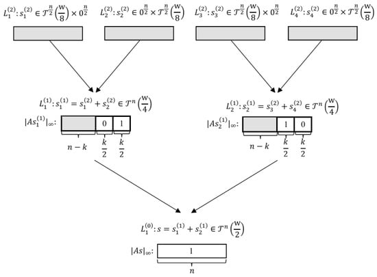
Figure 1. The tree structure of Rep-0. The shaded regions represent the parts where the matching operation has not been performed.

The merge process proceeds level by level. At each step, we perform both exact matching and approximate matching, employing the LSH-Odlyzko method from Section 2.3 for the latter. To ensure that expect one solution survives after merging, the parameter k must satisfy $q^{{\displaystyle \frac{k}{2}}}{\left({\displaystyle \frac{q}{3}}\right)}^{{\displaystyle \frac{k}{2}}}\approx R$. More precisely, k is calculated as

$$k=⌊{\displaystyle \frac{{log}_{2}R}{{log}_{2}q-0.5{log}_{2}3}}⌋.$$

(14)

The pseudocode of Rep-0 is presented in Algorithm 2.

Algorithm 2 Rep-0

Input: An LWE public key $(A,b)\in {\mathbb{Z}}_q^{n\times n}\times {\mathbb{Z}}_q^n$, weight w

Output: Secret vector $s\in {\mathcal{T}}^n(w/2)$ satisfying $As-bmodq\in {\mathcal{T}}^n$ of ⊥ if no such secret is found

1: Enumerate four level-2 lists $L_1^{\left(2\right)},L_2^{\left(2\right)},L_3^{\left(2\right)},L_4^{\left(2\right)}$ as above.

2: Choose k that satisfies $q^{{\displaystyle \frac{k}{2}}}{\left({\displaystyle \frac{q}{3}}\right)}^{{\displaystyle \frac{k}{2}}}\approx {\left({\displaystyle \genfrac{}{}{0pt}{}{w/2}{w/4}}\right)}^2$.

3: Merge $L_1^{\left(2\right)}$ and $L_2^{\left(2\right)}$ into $L_1^{\left(1\right)}$ using approximate matching on $k/2$ coordinates and exact matching on the other $k/2$ coordinates.

4: Merge $L_3^{\left(2\right)}$ and $L_4^{\left(2\right)}$ into $L_2^{\left(1\right)}$ similarly.

5: Merge $L_1^{\left(1\right)}$ and $L_2^{\left(1\right)}$ into $L_0^{\left(1\right)}$ using LSH on the remaining $n-k$ coordinates, and filter out any vector not in ${\mathcal{T}}^n(w/2)$.

6: If $L_1^{\left(0\right)}$ is non-empty, return any $s\in L_1^{\left(0\right)}$; otherwise, return ⊥.

After Step 3–4 in Algorithm 2, we obtain two level-1 lists with the following structure:

$$\begin{array}{cc}\hfill L_1^{\left(1\right)}& =\left\{s_1^{\left(1\right)}\in {\mathcal{T}}^n(w/4):A{s}_1^{\left(1\right)}\in {\mathbb{Z}}_q^{n-k}\times 0^{k/2}\times {\{\pm 1,0\}}^{k/2}\right\},\hfill \\ \hfill L_2^{\left(1\right)}& =\left\{s_2^{\left(1\right)}\in {\mathcal{T}}^n(w/4):A{s}_2^{\left(1\right)}\in {\mathbb{Z}}_q^{n-k}\times {\{\pm 1,0\}}^{k/2}\times 0^{k/2}\right\}.\hfill \end{array}$$

(15)

This means that vectors in $L_1^{\left(1\right)}$ satisfy $A{s}_1^{\left(1\right)}=0$ on $k/2$ coordinates (exact matching) and $A{s}_1^{\left(1\right)}\in \{\pm 1,0\}$ on another $k/2$ coordinates (approximate matching), while vectors in $L_2^{\left(1\right)}$ satisfy $A{s}_2^{\left(1\right)}\in \{\pm 1,0\}$ on $k/2$ coordinates and $A{s}_2^{\left(1\right)}=0$ on the other $k/2$ coordinates.

Step 5 in Algorithm 2 merges $L_1^{\left(1\right)}$ and $L_2^{\left(1\right)}$ using LSH-Odlyzko on the $n-k$ coordinates that were not involved in the previous matching steps. This finds pairs $(s_1^{\left(1\right)},s_2^{\left(1\right)})$ such that $A{s}_1^{\left(1\right)}$ and $b-A{s}_2^{\left(1\right)}$ are 1-close in the ${\ell }_{\infty }$-norm, which ensures that $s=s_1^{\left(1\right)}+s_2^{\left(1\right)}$ satisfies $As=b+e$ with $e\in {\mathcal{T}}^n$.

The correctness of Algorithm 2 follows from the representation technique: each valid secret s has multiple representations as $s_1^{\left(1\right)}+s_2^{\left(1\right)}$, and we expect that one of these representations survives the merging process. The LSH-based matching efficiently identifies pairs that satisfy Equation (12) without explicitly checking all possible pairs.

Let $L^{\left(j\right)}$ denote the common size of the lists at level j, for $j=0,1,2$. We have

$$\begin{array}{cc}\hfill L^{\left(2\right)}& =\left({\displaystyle \genfrac{}{}{0pt}{}{n/2}{w/8,w/8,·}}\right),\hfill \\ \hfill L^{\left(1\right)}& ={\left(L^{\left(2\right)}\right)}^2·{\left({\displaystyle \frac{3}{q}}\right)}^{{\displaystyle \frac{k}{2}}}·{\left({\displaystyle \frac{1}{q}}\right)}^{{\displaystyle \frac{k}{2}}},\hfill \\ \hfill L^{\left(0\right)}& ={\displaystyle \frac{{\left(L^{\left(1\right)}\right)}^2}{2^{n-k}}}.\hfill \end{array}$$

(16)

The space complexity is determined by the maximum list size encountered during the merging process:

$$S_{\mathrm{Rep}-0}=max\left\{L^{\left(2\right)},L^{\left(1\right)},L^{\left(0\right)}\right\}.$$

(17)

The time complexity is dominated by the largest list size and the cost of LSH-based merging at each level:

$$\begin{array}{cc}\hfill T_{\mathrm{Rep}-0}& =max\left\{S_{\mathrm{Rep}-0},T_{\mathsf{LSH}+\mathsf{Exact}}\left(L^{\left(2\right)},{\displaystyle \frac{k}{2}},{\displaystyle \frac{k}{2}},B\right),T_{\mathsf{LSH}+\mathsf{Exact}}\left(L^{\left(1\right)},n-k,0,{\displaystyle \frac{q}{2}}\right)\right\}\hfill \\ \hfill & =max\left\{S_{\mathrm{Rep}-0},{\left(L^{\left(2\right)}\right)}^2·{\left({\displaystyle \frac{B^2}{(B-1)q}}\right)}^{{\displaystyle \frac{k}{2}}}·{\left({\displaystyle \frac{1}{q}}\right)}^{{\displaystyle \frac{k}{2}}}·nlogn,{\displaystyle \frac{{\left(L^{\left(1\right)}\right)}^2·nlogn}{2^{n-k}}}\right\}.\hfill \end{array}$$

(18)

Here, the last equality follows from Equation (5). The bucket size B is a parameter that needs to be optimized.

3.2. Rep-1: Optimized LSH-Based MitM Attacks

Rep-1 generalizes Rep-0 by allowing more flexible decompositions. In addition to representing non-zero entries of s as sums of non-zero entries in $s_1^{\left(1\right)}$ and $s_2^{\left(1\right)}$, Rep-1 also allows zero entries in s to be represented as $1+(-1)$ or $(-1)+1$. This increases the number of representations and allows for a more efficient search tree.

We now describe Rep-1 with depth-3, as illustrated in Figure 2. The ternary LWE secret vector $s\in {\mathcal{T}}^n(w/2)$ is decomposed as

$$s=s_1^{\left(1\right)}+s_2^{\left(1\right)},\mathrm{where}{s}_1^{\left(1\right)}, s_2^{\left(1\right)}\in {\mathcal{T}}^n(w/4+\epsilon \left[1\right]).$$

(19)

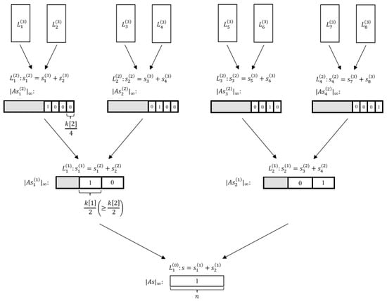
Figure 2. The tree structure of Rep-1 with depth 3. The shaded regions represent the parts where the matching operation has not been performed.

Here, $\epsilon \left[1\right]\ge 0$ is a parameter that controls the number of additional $\pm 1$ entries used to represent zeros in s. The total number of representations at level 1 is

$$R^{\left(1\right)}={\left({\displaystyle \genfrac{}{}{0pt}{}{w/2}{w/4}}\right)}^2·\left({\displaystyle \genfrac{}{}{0pt}{}{n-w}{\epsilon \left[1\right],\epsilon \left[1\right],·}}\right).$$

(20)

Each $s_i^{\left(1\right)}$ is further decomposed into two vectors at level 2:

$$s_i^{\left(1\right)}=s_{2i-1}^{\left(2\right)}+s_{2i}^{\left(2\right)},\mathrm{where}{s}_{2i-1}^{\left(2\right)}, s_{2i}^{\left(2\right)}\in {\mathcal{T}}^n\left({\displaystyle \frac{w}{8}}+{\displaystyle \frac{\epsilon \left[1\right]}{2}}+\epsilon \left[2\right]\right).$$

(21)

The number of representations at level 2 is

$$R^{\left(2\right)}={\left({\displaystyle \genfrac{}{}{0pt}{}{w/4+\epsilon \left[1\right]}{w/8+\epsilon \left[1\right]/2}}\right)}^2·\left({\displaystyle \genfrac{}{}{0pt}{}{n-w/2-2\epsilon \left[1\right]}{\epsilon \left[2\right],\epsilon \left[2\right],·}}\right).$$

(22)

Finally, at level 3, Rep-1 enumerates the vectors $s_j^{\left(3\right)}\in {\mathcal{T}}^{n/2}\left({\displaystyle \frac{w}{16}}+{\displaystyle \frac{\epsilon \left[1\right]}{4}}+{\displaystyle \frac{\epsilon \left[2\right]}{2}}\right)$ directly. The merging process uses a combination of exact and approximate matching at each level, with the number of matched coordinates $k\left[i\right]$ chosen to satisfy

$$k\left[i\right]=⌊{\displaystyle \frac{{log}_2{R}^{\left(i\right)}}{{log}_{2}q-{0.5}^i{log}_{2}3}}⌋.$$

(23)

The pseudocode of Rep-1 is outlined in Algorithm 3.

Algorithm 3 Rep-1 with Depth 3

Input: An LWE public key $(A,b)\in {\mathbb{Z}}_q^{n\times n}\times {\mathbb{Z}}_q^n$, weight w

Output: Secret vector $s\in {\mathcal{T}}^n(w/2)$ satisfying $As-bmodq\in {\mathcal{T}}^n$ of ⊥ if no such secret is found

1: Enumerate eight level-3 lists $L_1^{\left(3\right)},\dots ,L_8^{\left(3\right)}$ with weights as above.

2: Compute $k\left[2\right]$ from $R^{\left(2\right)}$ and merge pairs into four level-2 lists using exact and approximate matching.

3: Compute $k\left[1\right]$ from $R^{\left(1\right)}$ and merge into two level-1 lists using exact and approximate matching.

4: Merge level-1 lists into $L_1^{\left(0\right)}$ using LSH on the remaining $n-k\left[1\right]$ coordinates, and filter out any vector not in ${\mathcal{T}}^n(w/2)$.

5: If $L_1^{\left(0\right)}$ is non-empty, return any $s\in L_1^{\left(0\right)}$; otherwise, return ⊥.

Let $L^{\left(j\right)}$ denote the common size of the lists at level j, for $j=0,1,2,3$. We have

$$\begin{array}{cc}\hfill L^{\left(3\right)}& =\left({\displaystyle \genfrac{}{}{0pt}{}{n/2}{g(w,\epsilon [1],\epsilon [2\left]\right),g(w,\epsilon [1],\epsilon [2\left]\right),·}}\right),\hfill \\ \hfill L^{\left(2\right)}& ={\left(L^{\left(3\right)}\right)}^2·{\left({\displaystyle \frac{3}{q}}\right)}^{{\displaystyle \frac{k\left[2\right]}{4}}}·{\left({\displaystyle \frac{1}{q}}\right)}^{{\displaystyle \frac{3k\left[2\right]}{4}}},\hfill \\ \hfill L^{\left(1\right)}& ={\left(L^{\left(2\right)}\right)}^2·{\left({\displaystyle \frac{3}{q}}\right)}^{{\displaystyle \frac{k\left[1\right]-k\left[2\right]}{2}}}·{\left({\displaystyle \frac{1}{q}}\right)}^{{\displaystyle \frac{k\left[1\right]-k\left[2\right]}{2}}},\hfill \\ \hfill L^{\left(0\right)}& ={\displaystyle \frac{{\left(L^{\left(1\right)}\right)}^2}{2^{n-k}}},\hfill \end{array}$$

(24)

where $g(x,y,z):=x/16+y/4+z/2$.

The space complexity is determined by the maximum list size encountered during the merging process:

$$S_{\mathrm{Rep}-1}=max\left\{L^{\left(3\right)},L^{\left(2\right)},L^{\left(1\right)},L^{\left(0\right)}\right\}.$$

(25)

The time complexity is dominated by the largest list size and the cost of LSH-based merging at each level:

$$T_{\mathrm{Rep}-1}=max\left\{T^{\left(3\right)},T^{\left(2\right)},T^{\left(1\right)},T^{\left(0\right)}\right\},$$

(26)

where $T^{\left(i\right)}$ is the cost at level i for $i=0,1,2,3$,

$$\begin{array}{cc}\hfill T^{\left(3\right)}& =L^{\left(3\right)},\hfill \\ \hfill T^{\left(2\right)}& =max\left\{L^{\left(3\right)},L^{\left(2\right)},{\left(L^{\left(2\right)}\right)}^2·{\left({\displaystyle \frac{B{\left[2\right]}^2}{\left(B\right[2]-1)q}}\right)}^{{\displaystyle \frac{k\left[2\right]}{4}}}·{\left({\displaystyle \frac{1}{q}}\right)}^{{\displaystyle \frac{3k\left[2\right]}{4}}}·nlogn\right\},\hfill \\ \hfill T^{\left(1\right)}& =max\left\{L^{\left(2\right)},L^{\left(1\right)},{\left(L^{\left(1\right)}\right)}^2·{\left({\displaystyle \frac{B{\left[1\right]}^2}{\left(B\right[1]-1)q}}\right)}^{{\displaystyle \frac{k\left[1\right]-k\left[2\right]}{2}}}·{\left({\displaystyle \frac{1}{q}}\right)}^{{\displaystyle \frac{k\left[1\right]-k\left[2\right]}{2}}}·nlogn\right\},\hfill \\ \hfill T^{\left(0\right)}& =max\left\{L^{\left(1\right)},L^{\left(0\right)},{\displaystyle \frac{{\left(L^{\left(1\right)}\right)}^2}{2^{n-k}}}\right\}.\hfill \end{array}$$

(27)

The parameters $\epsilon \left[1\right], \epsilon \left[2\right], B\left[1\right], B\left[2\right]$ are optimized to minimize the overall complexity.

4. LSH-Based MitM Attacks on Ternary LWE via Quantum Walks

In this work, we develop new LSH-based MitM quantum algorithms for ternary LWE, which transform the key recovery problem into a graph search task amenable to quantum walks. We first present QRep-0, the quantum adaptation of Rep-0, to establish the foundational approach. We then introduce QRep-1, which builds upon Rep-1 and achieves a lower complexity through enhanced representation techniques.

4.1. QRep-0: Foundational Instantiation of LSH-Based MitM Quantum Algorithms

The ternary LWE problem aims to recover a ternary secret vector $s\in {\mathcal{T}}^n(w/2)$ satisfying $As=b+emodq$, with a ternary error vector e. We cast this cryptographic recovery problem as a graph search task solvable by quantum walks, where marked vertices represent valid LWE solutions.

Rep-0 features a level-2 search tree, as illustrated in Figure 1. The quantum walk operates on a graph constructed as the Cartesian product of four identical Johnson graphs. The construction begins with the four level-2 lists $L_j^{\left(2\right)}(1\le j\le 4)$, each of size $L^{\left(2\right)}=\left({\displaystyle \genfrac{}{}{0pt}{}{n/2}{w/8,w/8,·}}\right)$. From these, we define restricted subsets $U_j^{\left(2\right)}\subseteq L_j^{\left(2\right)}$ of size $U^{\left(2\right)}:={\left(L^{\left(2\right)}\right)}^{\gamma }$, where $\gamma \in [0,1]$ is a parameter to be optimized. Setting $N=L^{\left(2\right)}$ and $k=U^{\left(2\right)}$, the graph is formally given by

$$G_{\mathrm{QRep}-0}(V_{\mathrm{QRep}-0},E_{\mathrm{QRep}-0}):=J(N,k)\times J(N,k)\times J(N,k)\times J(N,k).$$

(28)

Each vertex $u\in V_{\mathrm{Rep}-0}$ is a 4-tuple $(U_1^{\left(2\right)},U_2^{\left(2\right)},U_3^{\left(2\right)},U_4^{\left(2\right)})$. Two vertices u and v are adjacent if and only if, for some index j, the components $U_j^{\left(2\right)}$ of u and v differ by exactly one element, while the other three components are identical.

The data structure associated with a vertex in $G_{\mathrm{QRep}-0}$ comprises all intermediate lists $U_j^{\left(i\right)}$ generated during the execution of Rep-0, which takes the vertex’s 4-tuple $(U_1^{\left(2\right)},\dots ,U_4^{\left(2\right)})$ as its level-2 input lists. Here, $U_j^{\left(i\right)}$ corresponds to the j-th list at level-i, for $0\le i\le 1$ and $1\le j\le 2^i$.

A vertex is marked if its resultant top-level list $U_1^{\left(0\right)}$ contains at least one valid ternary secret s satisfying $s\in {\mathcal{T}}^n(w/2)$ and $As-bmodq\in {\mathcal{T}}^n$. This direct correspondence guarantees that finding any marked vertex solves the original LWE problem.

We begin by explaining the role of the parameter $\gamma$: it governs the trade-off between the setup cost of QRep-0 and the cost of the quantum walk required to reach a marked vertex.

When $\gamma$ is large (close to 1), the setup cost dominates the overall complexity. In the extreme case of $\gamma =1$, all vertices become marked (since $U^{\left(2\right)}=L^{\left(2\right)}$), and QRep-0 reduces to the classical Rep-0 method, no longer relying on quantum walk.

Conversely, when $\gamma$ is small (close to 0), the setup cost is minimized, but the fraction of marked vertices becomes negligible. As a result, the cost of amplifying these marked vertices via quantum walk becomes the dominant factor in the overall complexity.

We now analyze the quantum resources—specifically, circuit width and depth—required by QRep-0 as detailed in Algorithm 4.

Algorithm 4 QRep-0

Input: An LWE public key $(A,b)$, weight w

Output: Secret vector $s\in {\mathcal{T}}^n(w/2)$ satisfying $As-bmodq\in {\mathcal{T}}^n$ or ⊥ if no such secret is found.

1: Prepare the initial state (normalization omitted): $$\sum _{u\in V_{\mathrm{Rep}-0}}|u⟩|p_u⟩|d\left(u\right)⟩.$$

2: Repeat $t_1=\mathcal{O}(1/\sqrt{ϵ})$ times:

(2.1) Apply the phase flip if u is marked: $$|u⟩|p_u⟩|d\left(u\right)⟩\mapsto \left\{\begin{array}{c}-|u⟩|p_u⟩|d\left(u\right)⟩, \mathrm{if} u \mathrm{is} \mathrm{marked},\hfill \\ |u⟩|p_u⟩|d\left(u\right)⟩, \hspace{0.17em}\mathrm{otherwise}.\hfill \end{array}\right.$$

(2.2) Perform the quantum walk for $t_2=\mathcal{O}(1/\sqrt{\delta })$ steps.

3: Measure the register $\left|d\right(u)⟩.$

4: If $U_1^{\left(0\right)}$ is non-empty, return any $s\in U_1^{\left(0\right)}$; otherwise, return ⊥.

Let $U^{\left(i\right)}$ denote the size of level-i lists in QRep-0, for $i=0,1$. These sizes follow the recurrence relations:

$$\begin{array}{cc}\hfill U^{\left(2\right)}& ={\left(L^{\left(2\right)}\right)}^{\gamma }={\left({\displaystyle \genfrac{}{}{0pt}{}{n/2}{w/8,w/8,·}}\right)}^{\gamma },\hfill \\ \hfill U^{\left(1\right)}& ={\left(U^{\left(2\right)}\right)}^2·{\left({\displaystyle \frac{3}{q}}\right)}^{{\displaystyle \frac{k}{2}}}·{\left({\displaystyle \frac{1}{q}}\right)}^{{\displaystyle \frac{k}{2}}},\hfill \\ \hfill U^{\left(0\right)}& ={\displaystyle \frac{{\left(U^{\left(1\right)}\right)}^2}{2^{n-k}}}.\hfill \end{array}$$

(29)

The quantum circuit width, which corresponds to the space complexity, is determined by three registers: the vertex register $|u⟩$ encoding a 4-tuple of subsets $(U_1^{\left(2\right)},\dots ,U_4^{\left(2\right)})$, requiring $4U^{\left(2\right)}$ qubits; the coin register $|p_u⟩$ of similar size; and the data register $\left|d\right(u)⟩$, which dominates the space complexity with $2U^{\left(1\right)}+U^{\left(0\right)}$ qubits. Hence, the overall circuit width (space complexity) is given by

$$S_{\mathrm{QRep}-0}=\mathcal{O}\left(max\left\{U^{\left(2\right)},U^{\left(1\right)},U^{\left(0\right)}\right\}\right).$$

(30)

The circuit depth, which corresponds to the time complexity, follows the quantum walk complexity:

$$T_{\mathrm{QRep}-0}=T_S+{\displaystyle \frac{1}{\sqrt{ϵ}}}\left({\displaystyle \frac{1}{\sqrt{\delta }}}{T}_U+T_C\right),$$

(31)

where $T_S$ encompasses the initial state preparation and data structure construction, $T_U$ captures the cost per quantum walk step including data updates, and $T_C=\mathcal{O}\left(1\right)$ represents the phase oracle for marked vertices.

From Equation (11), the spectral gap of $G_{\mathrm{QRep}-0}$ is

$$\delta =\Omega \left({\displaystyle \frac{1}{k}}\right)=\Omega \left({\displaystyle \frac{1}{U^{\left(2\right)}}}\right).$$

(32)

Since the classical Rep-0 algorithm yields, in expectation, a single element in $L_1^{\left(0\right)}$, the fraction of marked vertices $ϵ$ corresponds to the probability that all four subsets $U_j^{\left(2\right)}$ contain the necessary elements to reconstruct s. This fraction is given by

$$ϵ={\left({\displaystyle \frac{U^{\left(2\right)}}{L^{\left(2\right)}}}\right)}^4={\left(L^{\left(2\right)}\right)}^{4(\gamma -1)}.$$

(33)

To determine the circuit depth, we analyze the setup cost $T_S$ and update cost $T_U$ for the quantum walk in QRep-0. Following the methodology in Section 6 of [24], these costs correspond to the classical computational complexity of constructing and updating the hierarchical data structure used in Rep-0.

The setup cost $T_S$ involves creating the hierarchical lists according to Rep-0. The level-2 lists $U_j^{\left(2\right)}$ (for $j=1,2,3,4$) are constructed by randomly sampling $U^{\left(2\right)}$ elements from $L_j^{\left(2\right)}$. The level-1 lists such as $U_1^{\left(1\right)}$ are formed by mergeing $U_1^{\left(2\right)}$ and $U_2^{\left(2\right)}$ via exact matching and LSH. Finally, the level-0 list $U_1^{\left(0\right)}$ is built from the two level-1 lists using LSH. Therefore,

$$\begin{array}{cc}\hfill T_S& =max\left\{S_{\mathrm{QRep}-0},T_{\mathsf{LSH}+\mathsf{Exact}}\left(U^{\left(2\right)},{\displaystyle \frac{k}{2}},{\displaystyle \frac{k}{2}},B\right),T_{\mathsf{LSH}+\mathsf{Exact}}\left(U^{\left(1\right)},n-k,0,{\displaystyle \frac{q}{2}}\right)\right\}\hfill \\ \hfill & =max\left\{S_{\mathrm{QRep}-0},{\left(U^{\left(2\right)}\right)}^2·{\left({\displaystyle \frac{B^2}{(B-1)q}}\right)}^{{\displaystyle \frac{k}{2}}}·{\left({\displaystyle \frac{1}{q}}\right)}^{{\displaystyle \frac{k}{2}}}·nlogn,{\displaystyle \frac{{\left(U^{\left(1\right)}\right)}^2·nlogn}{2^{n-k}}}\right\}.\hfill \end{array}$$

(34)

The update cost $T_U$ involves involves inserting or deleting an element from one of the level-2 lists. Without loss of generality, we assume the element to be updated, denoted as x, belongs to $U_1^{\left(2\right)}$. The update of x in $U_1^{\left(2\right)}$ can be performed in time $\mathcal{O}\left(1\right)$.

The insertion or deletion of x subsequently triggers updates in the level-1 list $U_1^{\left(1\right)}$, which is formed by merging $U_1^{\left(2\right)}$ and $U_2^{\left(2\right)}$. Specifically, this requires inserting or deleting all elements $z\in U_1^{\left(1\right)}$ that are constructed by pairing x with some $y\in U_2^{\left(2\right)}$, where x and y satisfy the matching conditions on k coordinates: approximate matching on $k/2$ coordinates and exact matching on the other $k/2$ coordinates.

To analyze the number of such elements y (and thus the corresponding z) and the time complexity of locating them, we employ the following theorem:

Theorem 2.

Given an element $x\in {\mathbb{Z}}_q^n$ and a list L of size $\left|L\right|$ with independent and identically distributed elements drawn uniformly from ${\mathbb{Z}}_q^n$, there exists a classical algorithm that can find a $(1-o(1\left)\right)$-fraction of $y\in L$ satisfying ${max}_{i\in I}|x_i-y_i|=1$ for some set I of size $k_1$ and ${max}_{i\in J}|x_i-y_i|=0$ for some set J of size $k_2$. The time complexity of this algorithm is

$$max\left\{\left|L\right|·{\left({\displaystyle \frac{3}{q}}\right)}^{k_1}·{\left({\displaystyle \frac{1}{q}}\right)}^{k_2},\left|L\right|·{\left({\displaystyle \frac{B^2}{(B-1)q}}\right)}^{k_1}·{\left({\displaystyle \frac{1}{q}}\right)}^{k_2}·nlogn,\right\}$$

(35)

where the first term corresponds to the expected number of elements y that meet the above conditions.

Proof. 

A detailed derivation of this result is provided in Appendix A.    □

Applying Theorem 2, the time required to update $U_1^{\left(1\right)}$ due to the modification of x is given by

$$T_U^{\left(1\right)}=max\left\{U^{\left(2\right)}·{\left({\displaystyle \frac{3}{q}}\right)}^{{\displaystyle \frac{k}{2}}}·{\left({\displaystyle \frac{1}{q}}\right)}^{{\displaystyle \frac{k}{2}}},U^{\left(2\right)}·{\left({\displaystyle \frac{B^2}{(B-1)q}}\right)}^{{\displaystyle \frac{k}{2}}}·{\left({\displaystyle \frac{1}{q}}\right)}^{{\displaystyle \frac{k}{2}}}·nlogn,\right\}$$

(36)

The number of elements $z\in U_1^{\left(1\right)}$ that need to be updated is $U^{\left(2\right)}·{(3/q)}^{k/2}·{(1/q)}^{k/2}$. For each such z, applying Theorem 2 again, the time required to update the level-0 list $U^{\left(0\right)}$ is $(U^{\left(1\right)}·nlogn)/2^{n-k}$. Therefore, the total update time for the level-0 list is

$$T_U^{\left(0\right)}=U^{\left(2\right)}·{\left({\displaystyle \frac{3}{q}}\right)}^{{\displaystyle \frac{k}{2}}}·{\left({\displaystyle \frac{1}{q}}\right)}^{{\displaystyle \frac{k}{2}}}·{\displaystyle \frac{U^{\left(1\right)}·nlogn}{2^{n-k}}}$$

(37)

Consequently, the overall update cost is given by

$$T_U=max\left\{\mathcal{O}\left(1\right),T_U^{\left(1\right)},T_U^{\left(0\right)}\right\}.$$

(38)

An important observation is that $T_S$ and $T_U$ satisfy the relation $T_S=U^{\left(2\right)}{T}_U$. Combining this observation with Equations (31)–(33) and $T_C=\mathcal{O}\left(1\right)$, we obtain the circuit depth (time complexity) of QRep-0:

$$\begin{array}{cc}\hfill T_{\mathrm{QRep}-0}& =T_S+{\displaystyle \frac{1}{\sqrt{ϵ}}}\left({\displaystyle \frac{1}{\sqrt{\delta }}}{T}_U+T_C\right)\hfill \\ \hfill & =\mathcal{O}\left(U^{\left(2\right)}{T}_U+{\left({\displaystyle \frac{L^{\left(2\right)}}{U^{\left(2\right)}}}\right)}^2\left(\sqrt{U^{\left(2\right)}}{T}_U+1\right)\right)\hfill \\ \hfill & ={\left(L^{\left(2\right)}\right)}^{\gamma }{T}_U+{\left(L^{\left(2\right)}\right)}^{2(1-\gamma )+{\displaystyle \frac{\gamma }{2}}}{T}_U.\hfill \end{array}$$

(39)

The parameter $\gamma$ is chosen to minimize the overall time complexity by balancing the two dominant terms in the expression: the setup cost ${\left(L^{\left(2\right)}\right)}^{\gamma }{T}_U$ and the cost of performing the quantum walk to find a marked vertex ${\left(L^{\left(2\right)}\right)}^{2(1-\gamma )+{\displaystyle \frac{\gamma }{2}}}{T}_U$.

To achieve this balance, we set the exponents of the two terms equal to each other:

$$\gamma =2(1-\gamma )+\gamma /2.$$

(40)

Solving this equation for $\gamma$ yields the optimal value $\gamma =4/5$.

4.2. Concrete Security Analysis of QRep-0

We now present the concrete security analysis of our foundational QRep-0 algorithm and compare it with the vHKM’s QRep-0. Table 1 evaluates both methods on major ternary-LWE-based cryptographic schemes that were also analyzed by van Hoof et al. [18], including NTRU variants (Encrypt and Prime), BLISS signatures, and GLP signatures. These schemes all rely on the hardness of ternary LWE, where both the secret and error vectors have entries in $\{-1,0,1\}$.

Table 1. Comparative analysis of bit complexity: our QRep-0 vs. vHKM’s QRep-0.

Scheme	Parameters	Our QRep-0	vHKM’s QRep-0 [18]
	$\mathbf{(}\mathit{n}\mathbf{,}\mathit{q}\mathbf{,}\mathit{w}\mathbf{)}$	${\mathbf{log}}_{\mathbf{2}}\mathit{T}$	${\mathbf{log}}_{\mathbf{2}}\mathit{T}$
NTRU-Enc	$(509,2048,254)$	212	230
	$(677,2048,254)$	241	254
	$(821,4096,510)$	390	425
	$(701,8192,468)$	347	377
NTRU-Prime	$(653,4621,288)$	251	271
	$(761,4591,286)$	273	284
	$(857,5167,322)$	319	322
BLISS I+II	$(512,\mathrm{12,289},154)$	194	174
GLP I	$(512,\mathrm{8,383,489},342)$	252	264

The parameter triple $(n,q,w)$ for each scheme specifies the polynomial dimension n (ring dimension), the modulus q, and the weight w (number of non-zero entries in the ternary secret vector). The complexity is measured in ${log}_{2}T$, where T represents the time complexity of the attack. For quantum walk-based combinatorial attacks, including both our approach and vHKM’s method, the time complexity T and quantum space complexity M (measured in qubits) are essentially equivalent, i.e., ${log}_{2}T={log}_{2}M$. This resource equivalence arises because both methods rely on quantum walks over Johnson graphs that require storing the entire quantum state during computation.

Table 1 provides concrete complexity estimates for QRep-0. Across all cryptographic schemes evaluated, our QRep-0 implementation demonstrates superior performance over the vHKM variant in all cases except for BLISS I+II. As will be shown subsequently, when enhanced with improved representation techniques, our quantum algorithm achieves comprehensive advantage over the vHKM approach.

As shown in Table 1, our QRep-0 implementation outperforms the vHKM variant in all cases except for BLISS I+II. As will be shown subsequently, when enhanced with improved representation techniques, our quantum algorithm achieves comprehensive advantage over the vHKM approach.

4.3. QRep-1: Improved LSH-Based MitM Quantum Algorithms

Following the introduction of the foundational instantiation, we proceed to QRep-1—a superior instantiation of our quantum algorithm which leverages a more powerful representation technique. In this instantiation, the depth of the search tree is also treated as an optimization parameter.

We begin by describing QRep-1 with a depth of 3; its search tree structure is illustrated in Figure 2. Since the top level (level 3) contains 8 lists, the quantum walk is performed on the Cartesian product of 8 identical Johnson graphs. Consider subsets $U_j^{\left(3\right)}\subseteq L_j^{\left(3\right)}$ of size $U^{\left(3\right)}={\left(L^{\left(3\right)}\right)}^{\gamma },$ where parameter $\gamma \in [0,1]$ balances the quantum walk cost.

The spectral gap of the graph $J^8(L^{\left(3\right)},U^{\left(3\right)})$ is $\Omega (1/U^{\left(3\right)})$, and the fraction of marked vertices is ${(U^{\left(3\right)}/L^{\left(3\right)})}^8$.

Analogously to Section 4.1, we can recursively derive the list sizes from level 2 down to level 0:

$$\begin{array}{cc}\hfill U^{\left(2\right)}& ={\left(U^{\left(3\right)}\right)}^2·{\left({\displaystyle \frac{3}{q}}\right)}^{{\displaystyle \frac{k\left[2\right]}{4}}}·{\left({\displaystyle \frac{1}{q}}\right)}^{{\displaystyle \frac{3k\left[2\right]}{4}}},\hfill \\ \hfill U^{\left(1\right)}& ={\left(U^{\left(2\right)}\right)}^2·{\left({\displaystyle \frac{3}{q}}\right)}^{{\displaystyle \frac{k\left[1\right]-k\left[2\right]}{2}}}·{\left({\displaystyle \frac{1}{q}}\right)}^{{\displaystyle \frac{k\left[1\right]-k\left[2\right]}{2}}},\hfill \\ \hfill U^{\left(0\right)}& ={\displaystyle \frac{{\left(U^{\left(1\right)}\right)}^2}{2^{n-k}}}.\hfill \end{array}$$

(41)

The space complexity of QRep-1 with depth 3 is

$$S_{\mathrm{QRep}-1}=\mathcal{O}\left(max\left\{U^{\left(3\right)},U^{\left(2\right)},U^{\left(1\right)},U^{\left(0\right)}\right\}\right).$$

(42)

Similarly, the setup cost of the quantum walk for QRep-1 with depth 3 is

$$T_S=max\left\{T_S^{\left(3\right)},T_S^{\left(2\right)},T_S^{\left(1\right)},T_S^{\left(0\right)}\right\},$$

(43)

where $T_S^{\left(i\right)}$ is the setup cost at level i for $i=0,1,2,3$,

$$\begin{array}{cc}\hfill T_S^{\left(3\right)}& =U^{\left(3\right)},\hfill \\ \hfill T_S^{\left(2\right)}& =max\left\{U^{\left(3\right)},U^{\left(2\right)},{\left(U^{\left(2\right)}\right)}^2·{\left({\displaystyle \frac{B{\left[2\right]}^2}{\left(B\right[2]-1)q}}\right)}^{{\displaystyle \frac{k\left[2\right]}{4}}}·{\left({\displaystyle \frac{1}{q}}\right)}^{{\displaystyle \frac{3k\left[2\right]}{4}}}·nlogn\right\},\hfill \\ \hfill T_S^{\left(1\right)}& =max\left\{U^{\left(2\right)},U^{\left(1\right)},{\left(U^{\left(1\right)}\right)}^2·{\left({\displaystyle \frac{B{\left[1\right]}^2}{\left(B\right[1]-1)q}}\right)}^{{\displaystyle \frac{k\left[1\right]-k\left[2\right]}{2}}}·{\left({\displaystyle \frac{1}{q}}\right)}^{{\displaystyle \frac{k\left[1\right]-k\left[2\right]}{2}}}·nlogn\right\},\hfill \\ \hfill T_S^{\left(0\right)}& =max\left\{U^{\left(1\right)},U^{\left(0\right)},{\displaystyle \frac{{\left(U^{\left(1\right)}\right)}^2}{2^{n-k}}}\right\}.\hfill \end{array}$$

(44)

The parameters $\epsilon \left[1\right],\epsilon \left[2\right],B\left[1\right],B\left[2\right]$ are optimized to minimize the overall complexity.

The update cost of the quantum walk for QRep-1 with depth 3 is

$$T_U=max\left\{T_U^{\left(3\right)},T_U^{\left(2\right)},T_U^{\left(1\right)},T_U^{\left(0\right)}\right\},$$

(45)

where $T_U^{\left(i\right)}$ represents the update cost at level i for $i=0,1,2,3$.

Following an analysis similar to that in Section 4.1 and applying Theorem 2, we establish the relationship between the update cost and setup cost at each level: $T_S^{\left(i\right)}=U^{\left(3\right)}·T_U^{\left(i\right)}$, and consequently $T_S=U^{\left(3\right)}·T_U$. This relationship enables us to estimate the time complexity of QRep-1 as follows:

$$\begin{array}{cc}\hfill T_{\mathrm{QRep}-1}& =T_S+{\displaystyle \frac{1}{\sqrt{ϵ}}}\left({\displaystyle \frac{1}{\sqrt{\delta }}}{T}_U+T_C\right)\hfill \\ \hfill & =\mathcal{O}\left(U^{\left(3\right)}{T}_U+{\left({\displaystyle \frac{L^{\left(3\right)}}{U^{\left(3\right)}}}\right)}^4\left(\sqrt{U^{\left(3\right)}}{T}_U+1\right)\right)\hfill \\ \hfill & ={\left(L^{\left(3\right)}\right)}^{\gamma }{T}_U+{\left(L^{\left(3\right)}\right)}^{4(1-\gamma )+{\displaystyle \frac{\gamma }{2}}}{T}_U.\hfill \end{array}$$

(46)

Similarly, for QRep-1, we balance the setup cost ${\left(L^{\left(3\right)}\right)}^{\gamma }{T}_U$ and the search cost ${\left(L^{\left(3\right)}\right)}^{4(1-\gamma )+{\displaystyle \frac{\gamma }{2}}}{T}_U$ to find the optimal $\gamma$. The balancing equation is $\gamma =4(1-\gamma )+{\displaystyle \frac{\gamma }{2}}$. Solving this equation gives the optimal value $\gamma =8/9$.

A similar analysis at depth 4 gives $\gamma =16/17$. This demonstrates that the performance of QRep-1 converges to that of Rep-1 as the depth of the classical search tree increases.

4.4. Concrete Security Analysis of QRep-1

This subsection presents a comprehensive security analysis of our optimized QRep-1 algorithm, comparing it against previous quantum combinatorial attacks and lattice-based quantum sieving methods. Table 2 extends our evaluation to include additional ternary-LWE-based schemes from the NTRU-IEEE family, using the same methodology established in Section 4.2.

Table 2. Comparative analysis of bit complexity for ternary-LWE schemes.

Scheme	Parameters	vHKM’s QRep-1 [18]		Our QRep-1		Quantum Sieving † [25]
	$\mathbf{(}\mathit{n}\mathbf{,}\mathit{q}\mathbf{,}\mathit{w}\mathbf{)}$	${\mathbf{log}}_{\mathbf{2}}\mathit{T}$	${\mathbf{log}}_{\mathbf{S}}\mathit{T}$ *	${\mathbf{log}}_{\mathbf{2}}\mathit{T}$	${\mathbf{log}}_{\mathcal{S}}\mathit{T}$	${\mathbf{log}}_{\mathbf{2}}\mathit{T}$
NTRU-IEEE	(401, 2048, 226)	–	–	144	0.234	$70+c$
	(449, 2048, 268)	–	–	149	0.214	$82+c$
	(677, 2048, 314)	–	–	202	0.206	$134+c$
	(1087, 2048, 240)	–	–	220	0.207	$215+c$
	(541, 2048, 98)	–	–	113	0.244	$96+c$
	(613, 2048, 110)	–	–	132	0.254	$112+c$
	(887, 2048, 162)	–	–	169	0.221	$174+c$
	(1171, 2048, 212)	–	–	221	0.220	$243+c$
	(659, 2048, 76)	–	–	110	0.267	$118+c$
	(761, 2048, 84)	–	–	114	0.247	$140+c$
	(1087, 2048, 126)	–	–	167	0.245	$214+c$
	(1499, 2048, 158)	–	–	203	0.231	$300+c$
NTRU-Enc	(509, 2048, 254)	188	0.249	155	0.205	$95+c$
	(677, 2048, 254)	223	0.249	177	0.198	$133+c$
	(821, 4096, 510)	320	0.248	290	0.225	$159+c$
	(701, 8192, 468)	278	0.251	239	0.216	$122+c$
NTRU-Prime	(653, 4621, 288)	225	0.243	184	0.199	$116+c$
	(761, 4591, 286)	245	0.244	185	0.184	$139+c$
	(857, 5167, 322)	274	0.242	217	0.192	$158+c$
BLISS I+II	(512, 12,289, 154)	149	0.249	133	0.222	$79+c$
GLP I	(512, 8,383,489, 342)	193	0.240	169	0.210	$38+c$

* $\mathcal{S}$ is the size of the search space. ^† The term c denotes a constant in quantum sieving complexities.

All evaluated schemes rely on the hardness of ternary LWE with secret and error vectors restricted to $\{-1,0,1\}$ entries. The parameter triple $(n,q,w)$ for each scheme specifies the polynomial dimension, modulus, and weight of the secret vector, respectively. The complexity is measured in two forms: ${log}_{2}T$ represents the base-2 logarithm of the time complexity, while ${log}_{S}T$ expresses the time complexity relative to the search space size S, providing a normalized measure of efficiency.

Our QRep-1 algorithm achieves a concrete complexity bound of approximately ${\mathcal{S}}^{0.225}$, substantially improving upon the ${\mathcal{S}}^{0.251}$ bound of vHKM’s quantum combinatorial attack. This represents a significant reduction in the gap between asymptotic predictions and concrete performance. As shown in Table 2, our method demonstrates dramatic runtime improvements over vHKM, with speedup factors ranging from $2^{30}$ for NTRU-Enc-821 to $2^{60}$ for NTRU-Prime-761. For signature schemes, we observe speedups of $2^{16}$ for BLISS I+II and $2^{24}$ for GLP I.

The comparison with quantum sieving reveals a nuanced security landscape. While lattice-based attacks maintain advantages for most parameter sets, our combinatorial approach demonstrates superiority for small-weight parameters. This divergence highlights the importance of considering both attack paradigms in security assessments.

It is crucial to distinguish the resource models between these approaches. Quantum walk-based combinatorial attacks (including both our QRep-1 and vHKM’s) exhibit equivalence between time and quantum space complexity due to the quantum walk framework requiring storage of the entire quantum state. In contrast, quantum sieving employs a hybrid classical-quantum model where only the locality-sensitive filtering step is quantumized, resulting in a two-component resource model with both classical and quantum memory requirements.

Our combinatorial method leverages representation techniques derived from subset-sum or knapsack problems. This approach has strong theoretical foundations: for knapsack-type distributions, it can be rigorously proven that pathological instances constitute an exponentially small fraction, enabling the construction of provable probabilistic algorithms that avoid heuristics [15]. Experimental validation in prior work [15] confirms that observed runtimes align closely with theoretical predictions, providing enhanced precision in security estimates compared to lattice reduction heuristics that rely on unproven assumptions like the Geometric Series Assumption.

Our QRep-1 algorithm establishes the new state of the art for quantum combinatorial attacks on ternary LWE, offering both theoretical advances and practical security implications for post-quantum cryptography standardization.

5. LSH-Based MitM Quantum Algorithms with Polynomial Qubits

5.1. The Impact of Memory Models

Section 4 established the state of the art for quantum combinatorial attacks in terms of time complexity, operating under the strong QRAQM assumption. This model, which allows for coherent, efficient queries to an exponentially large quantum memory, is fundamental to the optimal performance of quantum walk-based approaches like our QRep0 and QRep1. However, the QRAQM model presents a significant barrier to practical implementability, as it requires maintaining and coherently manipulating a number of qubits that grows exponentially with the problem size—a requirement far beyond the capabilities of current and foreseeable quantum hardware due to constraints on qubit count, coherence time, and error rates.

In contrast, the QRACM model offers a more pragmatic alternative for early quantum cryptanalysis. The QRACM model assumes that large amounts of data can be stored in classical memory (which is cheap and abundant) and accessed in a quantum superposition—an operation often considered more feasible than full QRAQM. While this access may incur a polynomial overhead, it drastically reduces the quantum hardware requirements to only $\mathcal{O}\left(n\right)$ qubits. This distinction between QRAQM and QRACM is critical for assessing the practical viability of quantum algorithms. Our work directly addresses this implementability challenge by introducing a hybrid algorithm that functions efficiently under the more realistic QRACM assumption.

This leads to two distinct algorithmic paradigms for quantum combinatorial attacks: one prioritizing theoretical time efficiency (using quantum walks under QRAQM), and the other minimizing quantum hardware requirements for practical realization (using claw-finding under QRACM). The existence of this trade-off underscores that both asymptotic complexity and concrete resource constraints must be considered for a comprehensive security assessment.

Building on Benedikt’s [19] application of the Chailloux et al. [20] (CNPS) quantum claw-finding technique to ternary LWE, we extend this line of work through a novel integration with the Kirshanova–May [17] framework. This hybrid construction operates efficiently with only $\mathcal{O}\left(n\right)$ qubits under the QRACM model. We now detail this approach.

5.2. Reformulating LWE Key Recovery as a Consistent Claw-Finding Problem

Let $s\in {\mathcal{T}}^n(w/2)$ be a ternary LWE secret vector, and consider a representation $s=s_1+s_2$, where $s_1, s_2\in {\mathcal{T}}^n(w/4+\alpha )$ for some $\alpha \ge 0$. We rewrite the LWE identity given in Equation (12) for convenience:

$$A{s}_1=-A{s}_2+b+emodq.$$

(47)

Let $S_1, S_2\subseteq {\mathcal{T}}^n$. We define a pair of random, efficiently computable functions $f_1:S_1\to {\mathbb{Z}}_q^n$ and $f_2:S_2\to {\mathbb{Z}}_q^n$ (i.e., $T_{f_i}=\mathrm{poly}\left(n\right)$) given by

$$f_1:s_1\mapsto A{s}_{1}modq\mathrm{and}{f}_2:s_2\mapsto b-A{s}_{2}modq.$$

(48)

A 1-close claw for $f_1,f_2$ is defined as a pair $(s_1,s_2)\in S_1\times S_2$ that satisfies $\parallel f_1\left(s_1\right)-f_2\left(s_2\right){\parallel }_{\infty }=1$.

While every representation of the secret s yields a 1-close claw, the converse is not true: a 1-close claw pair does not necessarily satisfy $s_1+s_2\in {\mathcal{T}}^n(w/2)$. Define a 1-close claw pair $(s_1,s_2)$ as consistent when $s_1+s_2\in {\mathcal{T}}^n(w/2)$. The representation of s is then in one-to-one correspondence with a consistent 1-close claw $(s_1,s_2)$.

Consequently, the problem of recovering LWE secret s reduces to finding a consistent 1-close claw. The CNPS algorithm serves as an effective approach for solving the claw finding problem, as it utilizes only $O\left(n\right)$ qubits, which aligns with our objectives. We now present a variant of CNPS, recently proposed by Benedikt and tailored for addressing the LWE problem, as detailed in Algorithm 5.

Algorithm 5 Quantum Consistent 1-Close Claw Finding

Input: Random functions $f_1:s_1\mapsto A{s}_1 mod q$ and $f_2:s_2\mapsto b-A{s}_2 mod q$

Output: A consistent 1-close claw $(s_1,s_2)$

1: Define $S_r^{f_i}:=\{s_i\in S_i\mid f_i\left(s_i\right)=0 mod q^r\}$ for $i=1,2$.

Construct a sorted list (by the second entry): $$L=\{(s_1,f_1\left(s_1\right))\in S_r^{f_1}\times {\mathbb{Z}}_q^n\}\mathrm{with}\left|L\right|=2^{\ell }.$$

2: Execute amplitude amplification using the following subroutines:

(2.1) $\mathcal{A}$: Prepare the quantum state $$|{\varphi }_r⟩ :={\displaystyle \frac{1}{\sqrt{|S_r^{f_2}|}}}\sum _{x_2\in S_r^{f_2}}|s_2,f_2\left(s_2\right)⟩|0⟩.$$

(2.2) $O_{f_L}$: Apply the set-membership oracle $O_{f_L}$ $$O_{f_L}\left(\right|{\varphi }_r⟩) :={\displaystyle \frac{1}{\sqrt{|S_r^{f_2}|}}}\sum _{x_2\in S_r^{f_2}}|s_2,f_2\left(s_2\right)⟩|f_L\left(s_2\right)⟩,$$

where $$f_L\left(s_2\right):=\left\{\begin{array}{cc}1\hfill & \mathrm{if}\exists (s_1,f_1\left(s_1\right))\in L\mathrm{s}.\mathrm{t}.f_1\left(s_1\right)=f_2\left(s_2\right)\wedge s_1+s_2\in {\mathcal{T}}^n\left({\displaystyle \frac{w}{2}}\right)\hfill \\ 0\hfill & \mathrm{else}\hfill \end{array}\right..$$

3: Amplitude amplification eventually yields a state $|s_2,f_2\left(s_2\right)⟩|1⟩$. Measure this state.

4: For the measured $s_2$, search for a corresponding $s_1$ such that $(s_1,s_2)$ forms a consistent 1-close claw.

Algorithm 5 identifies a consistent 1-close claw $(s_1,s_2)$ with $O\left(n\right)$ qubits in two phases. First, it constructs a classically sorted list L. Then, it applies amplitude amplification to process a superposition of $s_2$ candidates. A set-membership oracle for L is used to find an L-suitable $s_2$, i.e., one for which a corresponding $s_1$ exists such that $(s_1,f_1\left(s_1\right))\in L$ and $(s_1,s_2)$ constitute a consistent 1-close claw.

Let R denote the number of consistent 1-close claws. The parameter r must satisfy the constraint $r\le {log}_{q}R$ to guarantee the existence of at least one claw satisfying $f_1\left(s_1\right)=0mod{q}^r$. Since a uniformly random $s_1\in S_1$ can be extended to a consistent 1-close claw with probability $R/|S_1|$, the list size parameter ℓ must consequently satisfy $2^{\ell }\ge \left|S_1\right|/R$.

Regarding the construction of the classic list L, the original CNPS algorithm builds the list in an element-wise manner using Grover search. However, Benedikt observed that Grover search offers no asymptotic advantage when multiple solutions are required. Consequently, his method employs a classical algorithm proposed by May to construct L. To achieve more accurate security estimates for practical cryptographic schemes, we adopt the LSH-based MitM technique introduced by Kirshanova and May for building L.

Recall the search tree structure of Rep-0 and Rep-1 from Section 3. We can set $L:=L_1^{\left(1\right)}$ and $S_r^{f_2}:=\{s_2\mid (s_2,f_2\left(s_2\right))\in L_2^{\left(1\right)}\}$. This ensures that $L_1^{\left(1\right)}$ contains at least one pair $(s_1,f_1\left(s_1\right))$, and the set derived from $L_2^{\left(1\right)}$ contains a $L_1^{\left(1\right)}$-suitable $s_2$ such that $(s_1,s_2)$ forms a consistent 1-close claw.

5.3. Quantum Consistent 1-Close Claw Finding for Rep-0

To make the better use of the representation technique, we reduce the size of list L by narrowing the search space for $s_1$. This is accomplished by adjusting the weight constraints to $L_1^{\left(1\right)}\subseteq S_1={\mathcal{T}}^n(cw/4)$ and $L_2^{\left(1\right)}\subseteq S_2={\mathcal{T}}^n((2-c)w/4)$, where $c\in [0,1]$. Consequently, the number of representations becomes

$$R_{\mathrm{Rep}-0}:={\left({\displaystyle \genfrac{}{}{0pt}{}{w/2}{cw/4}}\right)}^2.$$

(49)

With this adjustment, the sizes of the level-2 and level-1 lists are given as follows:

$$\begin{array}{cc}\hfill |L_1^{\left(2\right)}|=|L_2^{\left(2\right)}|& =\left({\displaystyle \genfrac{}{}{0pt}{}{n/2}{cw/8,cw/8,·}}\right),\hfill \\ \hfill |L_3^{\left(2\right)}|=|L_4^{\left(2\right)}|& =\left({\displaystyle \genfrac{}{}{0pt}{}{n/2}{(2-c)w/8,(2-c)w/8,·}}\right),\hfill \\ \hfill |L_1^{\left(1\right)}|& = |L_1^{\left(2\right)}|·|L_2^{\left(2\right)}|·{\left({\displaystyle \frac{3}{q}}\right)}^{{\displaystyle \frac{k}{2}}}·{\left({\displaystyle \frac{1}{q}}\right)}^{{\displaystyle \frac{k}{2}}},\hfill \\ \hfill |L_2^{\left(1\right)}|& = |L_3^{\left(2\right)}|·|L_4^{\left(2\right)}|·{\left({\displaystyle \frac{3}{q}}\right)}^{{\displaystyle \frac{k}{2}}}·{\left({\displaystyle \frac{1}{q}}\right)}^{{\displaystyle \frac{k}{2}}}.\hfill \end{array}$$

(50)

The corresponding parameter k satisfies

$$k=⌊{\displaystyle \frac{{log}_2{R}_{\mathrm{Rep}-0}}{{log}_{2}q-0.5{log}_{2}3}}⌋.$$

(51)

It follows that

$$2^{\ell }=\left|L_1^{\left(1\right)}\right|=\left({\displaystyle \genfrac{}{}{0pt}{}{n}{cw/4,cw/4,·}}\right)·{\left({\displaystyle \frac{3}{q}}\right)}^{{\displaystyle \frac{k}{2}}}·{\left({\displaystyle \frac{1}{q}}\right)}^{{\displaystyle \frac{k}{2}}}\ge {\displaystyle \frac{|{\mathcal{T}}^n(cw/4)|}{R_{\mathrm{Rep}-0}}}={\displaystyle \frac{|S_1|}{R_{\mathrm{Rep}-0}}},$$

(52)

which is the constraint that the parameter ℓ must satisfy.

Using Rep-0, the list $L=L_1^{\left(1\right)}$ is constructed classically, requiring time and space complexities of

$$T_1=max\left\{|L_1^{\left(2\right)}|,|L_1^{\left(1\right)}|,T_{\mathsf{LSH}+\mathsf{Exact}}\left(|L_1^{\left(2\right)}|,{\displaystyle \frac{k}{2}},{\displaystyle \frac{k}{2}},B\right)\right\};M_1=max\left\{|L_1^{\left(2\right)}|,|L_1^{\left(1\right)}|\right\}.$$

(53)

Let $r:={log}_q{R}_{\mathrm{Rep}-0}$. In Step 2.1 of Algorithm 5, subroutine $\mathcal{A}$ begins by preparing a uniform superposition over $S_2$, which corresponds to a ternary Dicke state. This state can be constructed using $\mathcal{O}\left(n\right)$ qubits in linear time. Subsequently, $\mathcal{A}$ executes a Grover search—without the final measurement—to generate the state $|{\varphi }_r⟩$. The overall qubit requirement for $\mathcal{A}$ remains $\mathcal{O}\left(n\right)$. Due to the randomness of $f_2$, any $s_2\in S_2$ satisfies $f_2\left(s_2\right)=0mod{q}^r$ with probability $q^{-r}$, leading to a runtime of

$$T_{\mathcal{A}}=\mathcal{O}\left(q^{r/2}\right)=\sqrt{R_{\mathrm{Rep}-0}}.$$

(54)

For Step 2.2 of Algorithm 5, the quantum set-membership oracle for L operates with time complexity $T_{f_L}=\mathcal{O}(n·2^{\ell })=\mathcal{O}(n·|L_1^{\left(1\right)}\left|\right)$ and utilizes $2n+1$ qubits [19].

A uniformly random $s_1\in S_1$ can be extended to a consistent 1-close claw $(s_1,s_2)$ with probability $R_{\mathrm{Rep}-0}/\left|S_1\right|$. This probability distribution remains unchanged when sampling from $S_r^{f_1}$. Consequently, the expected number of consistent 1-close claws $(s_1,s_2)$ with $(s_1,f_1\left(s_1\right))\in L$ is $\left|L\right|·R_{\mathrm{Rep}-0}/\left|S_1\right|$. It follows that for any $x_2\in S_r^{f_2}$, the probability of $f_L\left(s_2\right)=1$ is given by

$$p={\displaystyle \frac{\left|L\right|·R_{\mathrm{Rep}-0}}{|S_r^{f_2}|·|S_1|}}={\displaystyle \frac{|L_1^{\left(1\right)}|·R_{\mathrm{Rep}-0}}{|L_2^{\left(1\right)}|·|S_1|}}={\displaystyle \frac{1}{|L_2^{\left(1\right)}|}}.$$

(55)

Applying Equation (6), the runtime complexity for Step 2 of Algorithm 5 becomes

$$T_2=\mathcal{O}\left({\displaystyle \frac{1}{\sqrt{p}}}·\left(T_{\mathcal{A}}+T_{f_L}\right)\right)=\mathcal{O}\left(\sqrt{|L_2^{\left(1\right)}|}·\left(\sqrt{R_{\mathrm{Rep}-0}}+n·\left|L_1^{\left(1\right)}\right|\right)\right).$$

(56)

The space requirement for this step is $\mathcal{O}\left(n\right)$ qubits.

Step 3 of Algorithm 5, which leverages the sorted structure of L, executes in time $\mathcal{O}\left(\ell \right)$. The overall time complexity of the algorithm for Rep-0 is therefore bounded by

$$T=\mathcal{O}\left(max\{T_1,T_2\}\right),$$

(57)

with total resource requirements of $\mathcal{O}\left(2^{\ell }\right)$ classical memory and $\mathcal{O}\left(n\right)$ qubits.

5.4. Concrete Security Analysis of Rep-0 Instantiation

We provide concrete complexity estimates for the quantum consistent 1-close claw finding subroutine (Rep-0 instantiation) in Table 3.

Table 3. Bit complexities for the quantum consistent 1-close claw finding subroutine (Rep-0 instantiation).

Scheme	Parameters	Time	Classical Memory
	$\mathbf{(}\mathit{n}\mathbf{,}\mathit{q}\mathbf{,}\mathit{w}\mathbf{)}$	${\mathbf{log}}_{\mathbf{2}}\mathit{T}$	${\mathbf{log}}_{\mathbf{2}}\mathit{M}$
NTRU-IEEE	(401, 2048, 226)	297	73
	(449, 2048, 268)	344	75
	(677, 2048, 314)	472	124
	(1087, 2048, 240)	526	50
	(541, 2048, 98)	239	0
	(613, 2048, 110)	265	17
	(887, 2048, 162)	383	34
	(1171, 2048, 212)	503	50
	(659, 2048, 76)	211	0
	(761, 2048, 84)	236	0
	(1087, 2048, 126)	349	19
	(1499, 2048, 158)	445	37
NTRU-Enc	(509, 2048, 254)	361	107
	(677, 2048, 254)	433	114
	(821, 4096, 510)	614	247
	(701, 8192, 468)	536	236
NTRU-Prime	(653, 4621, 288)	449	103
	(761, 4591, 286)	488	107
	(857, 5167, 322)	556	131
BLISS I+II	(512, 12,289, 154)	300	66
GLP I	(512, 8,383,489, 342)	387	200

The parameter triple $(n,q,w)$ for each scheme specifies the polynomial dimension, the modulus, and the weight of the secret vector, respectively. The complexity is measured in ${log}_{2}T$, where T represents the time complexity of the classical–quantum hybrid attack. The quantum space complexity, corresponding to the number of qubits required, is polynomial in n for all instances. The classical memory complexity, measured in ${log}_{2}M$, is often exponential; a value of 0 in Table 3 indicates that the required classical memory is polynomial.

We further consider the trade-off between time and classical memory. By constraining the available classical memory, we can optimize the time complexity of our algorithm. We present the trade-off curves for five representative examples, as shown in Figure 3. A similar analysis can be conducted for other parameter sets.

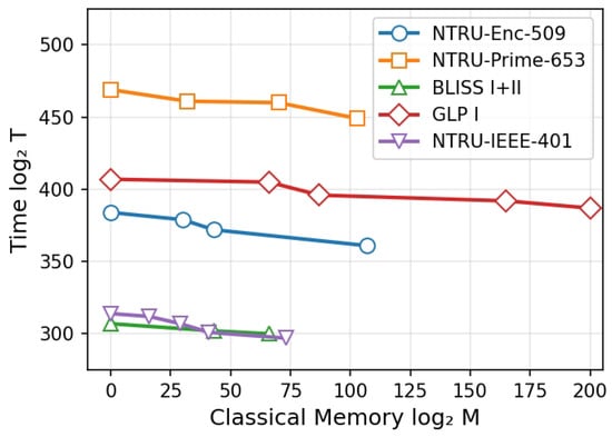
Figure 3. Time–classical memory trade-offs for five representative schemes under the Rep-0 instantiation.

5.5. Quantum Consistent 1-Close Claw Finding for Rep-1

Consider quantum consistent 1-close claw finding for Rep-1 with depth 3. Similar to Section 5.3, we adjusting the weight constraints to $L_1^{\left(1\right)}\subseteq S_1={\mathcal{T}}^n(cw/4+ϵ\left[1\right])$ and $L_2^{\left(1\right)}\subseteq S_2={\mathcal{T}}^n((2-c)w/4+ϵ\left[1\right])$, where $c\in [0,1]$. Consequently, the number of representations becomes

$$\begin{array}{cc}\hfill R_{\mathrm{Rep}-1}^{\left(1\right)}& :={\left({\displaystyle \genfrac{}{}{0pt}{}{w/2}{cw/4}}\right)}^2·\left({\displaystyle \genfrac{}{}{0pt}{}{n-w}{\epsilon \left[1\right],\epsilon \left[1\right],·}}\right),\hfill \\ \hfill R_{\mathrm{Rep}-1}^{\left(2\right)}& :={\left({\displaystyle \genfrac{}{}{0pt}{}{cw/4+\epsilon \left[1\right]}{cw/8+\epsilon \left[1\right]/2}}\right)}^2·\left({\displaystyle \genfrac{}{}{0pt}{}{n-w/2-2\epsilon \left[1\right]}{ϵ\left[2\right],ϵ\left[2\right],·}}\right).\hfill \end{array}$$

(58)

With this adjustment, the sizes of the level-i lists (for $1\le i\le 3$) are given as follows:

$$\begin{array}{cc}\hfill |L_j^{\left(3\right)}|& =\left({\displaystyle \genfrac{}{}{0pt}{}{n/2}{g(cw,\epsilon [1],\epsilon [2\left]\right),g(cw,\epsilon [1],\epsilon [2\left]\right),·}}\right),\mathrm{for}j=1,2,3,4,\hfill \\ \hfill |L_j^{\left(3\right)}|& =\left({\displaystyle \genfrac{}{}{0pt}{}{n/2}{g\left(\right(2-c)w,\epsilon [1],\epsilon [2\left]\right),g\left(\right(2-c)w,\epsilon [1],\epsilon [2\left]\right),·}}\right),\mathrm{for}j=5,6,7,8,\hfill \\ \hfill |L_j^{\left(2\right)}|& ={\left(|L_1^{\left(3\right)}|\right)}^2·{\left({\displaystyle \frac{3}{q}}\right)}^{{\displaystyle \frac{k\left[2\right]}{4}}}·{\left({\displaystyle \frac{1}{q}}\right)}^{{\displaystyle \frac{3k\left[2\right]}{4}}},\mathrm{for}j=1,2,\hfill \\ \hfill |L_j^{\left(2\right)}|& ={\left(|L_5^{\left(3\right)}|\right)}^2·{\left({\displaystyle \frac{3}{q}}\right)}^{{\displaystyle \frac{k\left[2\right]}{4}}}·{\left({\displaystyle \frac{1}{q}}\right)}^{{\displaystyle \frac{3k\left[2\right]}{4}}},\mathrm{for}j=3,4,\hfill \\ \hfill |L_1^{\left(1\right)}|& ={\left(|L_1^{\left(2\right)}|\right)}^2·{\left({\displaystyle \frac{3}{q}}\right)}^{{\displaystyle \frac{k\left[1\right]-k\left[2\right]}{2}}}·{\left({\displaystyle \frac{1}{q}}\right)}^{{\displaystyle \frac{k\left[1\right]-k\left[2\right]}{2}}},\hfill \\ \hfill |L_2^{\left(1\right)}|& ={\left(|L_3^{\left(2\right)}|\right)}^2·{\left({\displaystyle \frac{3}{q}}\right)}^{{\displaystyle \frac{k\left[1\right]-k\left[2\right]}{2}}}·{\left({\displaystyle \frac{1}{q}}\right)}^{{\displaystyle \frac{k\left[1\right]-k\left[2\right]}{2}}},\hfill \end{array}$$

(59)

where $g(x,y,z):=x/16+y/4+z/2$.

The corresponding parameter $k\left[i\right]$ (for $i=1,2$) satisfies

$$k\left[i\right]=⌊{\displaystyle \frac{{log}_2{R}_{\mathrm{Rep}-1}^{\left(i\right)}}{{log}_{2}q-0.5^i{log}_{2}3}}⌋.$$

(60)

Similarly, it follows that $2^{\ell }=|L_1^{\left(1\right)}|\ge |S_1|/R_{\mathrm{Rep}-1}^{\left(1\right)}$.

Using Rep-1, the list $L=L_1^{\left(1\right)}$ is constructed classically, requiring time and space complexity of

$$\begin{array}{c}{T}_1=max\{M_1,T_{\mathsf{LSH}+\mathsf{Exact}}\left(|L_1^{\left(3\right)}|,{\displaystyle \frac{k\left[2\right]}{4}},{\displaystyle \frac{3k\left[2\right]}{4}},B\left[2\right]\right),\hfill \\ \hfill T_{\mathsf{LSH}+\mathsf{Exact}}\left(|L_1^{\left(2\right)}|,{\displaystyle \frac{k\left[1\right]-k\left[2\right]}{2}},{\displaystyle \frac{k\left[1\right]-k\left[2\right]}{2}},B\left[1\right]\right)\},\end{array}$$

(61)

where $M_1=max\left\{|L_1^{\left(3\right)}|,|L_1^{\left(2\right)}|,|L_1^{\left(1\right)}|\right\}$ represents the classical memory.

Let $r:={log}_q{R}_{\mathrm{Rep}-1}^{\left(1\right)}$. Similar to the analysis from Section 5.3, we get

$$\begin{array}{cc}\hfill T_{\mathcal{A}}& =\mathcal{O}\left(q^{r/2}\right)=\sqrt{R_{\mathrm{Rep}-1}^{\left(1\right)}},\hfill \\ \hfill T_{f_L}& =\mathcal{O}(n·2^{\ell })=\mathcal{O}(n·|L_1^{\left(1\right)}|),\hfill \\ \hfill p& ={\displaystyle \frac{\left|L\right|·R_{\mathrm{Rep}-1}^{\left(1\right)}}{|S_r^{f_2}|·|S_1|}}={\displaystyle \frac{|L_1^{\left(1\right)}|·R_{\mathrm{Rep}-1}^{\left(1\right)}}{|L_2^{\left(1\right)}|·|S_1|}}={\displaystyle \frac{1}{|L_2^{\left(1\right)}|}}.\hfill \end{array}$$

(62)

Thus, the runtime complexity for Step 2 of Algorithm 5 becomes

$$T_2=\mathcal{O}\left({\displaystyle \frac{1}{\sqrt{p}}}·\left(T_{\mathcal{A}}+T_{f_L}\right)\right)=\mathcal{O}\left(\sqrt{|L_2^{\left(1\right)}|}·\left(\sqrt{R_{\mathrm{Rep}-1}^{\left(1\right)}}+n·\left|L_1^{\left(1\right)}\right|\right)\right).$$

(63)

The overall time complexity of Algorithm 5 for Rep-1 with depth 3 is therefore bounded by

$$T=\mathcal{O}\left(max\{T_1,T_2\}\right),$$

(64)

with total resource requirements of $\mathcal{O}\left(2^{\ell }\right)$ classical memory and $\mathcal{O}\left(n\right)$ qubits.

5.6. Concrete Security Analysis of Rep-1 Instantiation

We provide concrete complexity estimates for the quantum consistent 1-close claw finding subroutine (Rep-1 instantiation) in Table 4.

Table 4. Bit complexities for the quantum consistent 1-close claw finding subroutine (Rep-1 instantiation).

Scheme	Parameters	Time		Classical Memory
	$\mathbf{(}\mathit{n}\mathbf{,}\mathit{q}\mathbf{,}\mathit{w}\mathbf{)}$	${\mathbf{log}}_{\mathbf{2}}\mathit{T}$	${\mathbf{log}}_{\mathbf{S}}\mathit{T}$ *	${\mathbf{log}}_{\mathbf{2}}\mathit{M}$
NTRU-IEEE	(401, 2048, 226)	239	0.388	166
	(449, 2048, 268)	282	0.404	192
	(677, 2048, 314)	377	0.385	268
	(1087, 2048, 240)	421	0.397	321
	(541, 2048, 98)	186	0.403	127
	(613, 2048, 110)	217	0.413	157
	(887, 2048, 162)	303	0.396	185
	(1171, 2048, 212)	415	0.414	295
	(659, 2048, 76)	182	0.443	142
	(761, 2048, 84)	196	0.426	149
	(1087, 2048, 126)	291	0.427	192
	(1499, 2048, 158)	364	0.414	285
NTRU-Enc	(509, 2048, 254)	300	0.397	200
	(677, 2048, 254)	345	0.387	234
	(821, 4096, 510)	530	0.412	516
	(701, 8192, 468)	466	0.423	466
NTRU-Prime	(653, 4621, 288)	364	0.392	231
	(761, 4591, 286)	383	0.381	240
	(857, 5167, 322)	423	0.374	264
BLISS I+II	(512, 12,289, 154)	231	0.385	157
GLP I	(512, 8,383,489, 342)	328	0.408	238

* $\mathcal{S}$ is the size of the search space.

The parameter triple $(n,q,w)$ for each scheme specifies the polynomial dimension, modulus, and weight of the secret vector, respectively. The complexity is measured in two forms: ${log}_{2}T$ represents the base-2 logarithm of the time complexity, while ${log}_{S}T$ expresses the time complexity relative to the search space size S, providing a normalized measure of efficiency. The classical memory requirement is given by ${log}_{2}M$.

In the work of Benedikt [19], an asymptotic analysis of quantum claw-finding was provided for $w/n\in [0.375,0.668]$, concluding that the time complexity T falls within the range $[S^{0.379},S^{0.397}]$. In our concrete analysis shown in Table 4, for schemes where $w/n\in [0.375,0.668]$, the time complexity T ranges from $S^{0.381}$ to $S^{0.423}$, which aligns reasonably well with the asymptotic predictions, demonstrating the consistency between our concrete implementations and theoretical asymptotic analysis.

We further examine the trade-off between time and classical memory by optimizing the time complexity under constrained classical memory resources. Figure 4 illustrates this trade-off for five representative examples, showing how attack time varies with available classical memory. Similar analysis can be extended to other parameter sets, providing a comprehensive understanding of the resource-performance landscape.

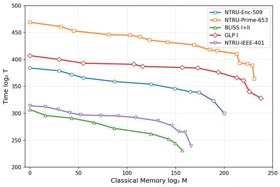
Figure 4. Time–classical memory trade-offs for five representative schemes under the Rep-1 instantiation.

Finally, we consider the scenario where both quantum and classical memory complexities are constrained to polynomial bounds. Table 5 compares our method with the vHKM [18] approach under such strict polynomial memory constraints. The results demonstrate that our algorithm achieves superior performance across all evaluated schemes, consistently requiring fewer computational resources than the vHKM method while maintaining the same polynomial memory footprint.

Table 5. Comparison of time complexity under polynomial memory.

Scheme	Parameters	vHKM  [18]	Ours
	$\mathbf{(}\mathit{n}\mathbf{,}\mathit{q}\mathbf{,}\mathit{w}\mathbf{)}$	${\mathbf{log}}_{\mathbf{2}}\mathit{T}$	${\mathbf{log}}_{\mathbf{2}}\mathit{T}$
NTRU-Enc	(509, 2048, 254)	401	384
	(677, 2048, 254)	463	454
	(821, 4096, 510)	708	650
	(701, 8192, 468)	620	558
NTRU-Prime	(653, 4621, 288)	486	469
	(761, 4591, 286)	521	510
	(857, 5167, 322)	586	574
BLISS I+II	(512, 12,289, 154)	309	307
GLP I	(512, 8,383,489, 342)	453	407

6. Conclusions

In this work, we have advanced the frontier of quantum combinatorial cryptanalysis for ternary LWE. We introduced a novel quantum key search algorithm that effectively addresses the critical limitation of prior quantum approaches—the costly need to guess error coordinates. By reformulating the problem as a graph search and integrating the classical LSH-based Meet-in-the-Middle framework of Kirshanova and May with a quantum walk, our attack achieves a significant reduction in concrete time complexity. This allows it to bridge the gap between the asymptotic promise of quantum combinatorial attacks and their practical performance, establishing a new state of the art. Our comprehensive security analysis provides revised, and more precise, quantum security estimates for a wide range of practical cryptographic schemes, including NTRU, BLISS, and GLP. The primary and most effective defense against the quantum combinatorial attacks presented in this work is to appropriately increase the size of the search space. This can be achieved by scaling parameters such as the polynomial dimension n or the weight w of the secret vector.

Furthermore, we addressed the critical issue of quantum resource constraints by presenting a second algorithm tailored for a polynomial-qubit setting. By combining the Kirshanova–May framework with a quantum claw-finding technique, we demonstrated that effective attacks remain feasible even with minimal quantum memory, albeit at the cost of increased classical storage and time. This analysis provides the first concrete security assessment of major schemes under such practical quantum hardware limitations.

References

- Regev, O. New lattice-based cryptographic constructions. J. ACM 2004, 51, 899–942. [Google Scholar] [CrossRef]
- Brakerski, Z.; Gentry, C.; Vaikuntanathan, V. (Leveled) fully homomorphic encryption without bootstrapping. ACM Trans. Comput. Theory 2014, 6, 1–36. [Google Scholar] [CrossRef]
- Bos, J.; Ducas, L.; Kiltz, E.; Lepoint, T.; Lyubashevsky, V.; Schanck, J.M.; Schwabe, P.; Seiler, G.; Stehlé, D. CRYSTALS-Kyber: A CCA-secure module-lattice-based KEM. In Proceedings of the 2018 IEEE European Symposium on Security and Privacy (EuroS&P), London, UK, 24–26 April 2018; pp. 353–367. [Google Scholar]
- Ducas, L.; Kiltz, E.; Lepoint, T.; Lyubashevsky, V.; Schwabe, P.; Seiler, G.; Stehlé, D. Crystals-dilithium: A lattice-based digital signature scheme. IACR Trans. Cryptogr. Hardw. Embed. Syst. 2018, 2018, 238–268. [Google Scholar] [CrossRef]
- Lyubashevsky, V.; Peikert, C.; Regev, O. On ideal lattices and learning with errors over rings. In Advances in Cryptology—EUROCRYPT 2010, Proceedings of the Annual International Conference on the Theory and Applications of Cryptographic Techniques, French Riviera, French, 30 May–3 June 2010; Springer: Berlin/Heidelberg, Germany, 2010; pp. 1–23. [Google Scholar]
- IEEE Std 1363.1-2008; IEEE Standard Specification for Public Key Cryptographic Techniques Based on Hard Problems over Lattices. IEEE: Piscataway, NJ, USA, 2009. Available online: https://ieeexplore.ieee.org/document/4800404 (accessed on 10 March 2009).
- Bernstein, D.J.; Chuengsatiansup, C.; Lange, T.; van Vredendaal, C. NTRU Prime: Reducing Attack Surface at Low Cost. In Selected Areas in Cryptography—SAC 2017, Proceedings of the SAC 2017, 24th International Conference, Ottawa, ON, Canada, 16–18 August 2017; Adams, C., Camenisch, J., Eds.; Lecture Notes in Computer Science; Springer: Cham, Switzerland, 2018; Volume 10719. [Google Scholar]
- Hülsing, A.; Rijneveld, J.; Schanck, J.; Schwabe, P. High-speed key encapsulation from NTRU. In Proceedings of the International Conference on Cryptographic Hardware and Embedded Systems, Taipei, Taiwan, 25–28 September 2017; Springer: Berlin/Heidelberg, Germany, 2017; pp. 232–252. [Google Scholar]
- Ducas, L.; Durmus, A.; Lepoint, T.; Lyubashevsky, V. Lattice signatures and bimodal Gaussians. In Advances in Cryptology, Proceedings of the CRYPTO 2013: Annual Cryptology Conference, Santa Barbara, CA, USA, 18–22 August 2013; Springer: Berlin/Heidelberg, Germany, 2013; pp. 40–56. [Google Scholar]
- Güneysu, T.; Lyubashevsky, V.; Pöppelmann, T. Practical lattice-based cryptography: A signature scheme for embedded systems. In Cryptographic Hardware and Embedded Systems—CHES 2012, Proceedings of the 14th International Workshop, Leuven, Belgium, 9–12 September 2012; Springer: Berlin/Heidelberg, Germany, 2012; Volume 7428, pp. 530–547. [Google Scholar]
- Hoffstein, J.; Pipher, J.; Silverman, J.H. NTRU: A ring-based public key cryptosystem. In Algorithmic Number Theory, Proceedings of the Third International Symposium, Portland, OR, USA, 21–25 June 1998; Buhler, J.P., Ed.; Springer: Berlin/Heidelberg, Germany, 1998; pp. 267–288. [Google Scholar]
- Howgrave-Graham, N. A hybrid lattice-reduction and meet-in-the-middle attack against NTRU. In Annual International Cryptology—CRYPTO 2007, Proceedings of the 27th Annual International Cryptology Conference, Santa Barbara, CA, USA, 19–23 August 2007; Springer: Berlin/Heidelberg, Germany, 2007; pp. 150–169. [Google Scholar]
- May, A. How to meet ternary LWE keys. In Advances in Cryptology—CRYPTO 2021, Proceedings of the 41st Annual International Cryptology Conference, Virtual Event, 16–20 August 2021; Springer International Publishing: Cham, Switzerland, 2021; pp. 701–731. [Google Scholar]
- Howgrave-Graham, N.; Joux, A. New generic algorithms for hard knapsacks. In Advances in Cryptology—EUROCRYPT 2010, Proceedings of the 29th Annual International Conference on the Theory and Applications of Cryptographic Techniques, French Riviera, French, 30 May–3 June 2010; Springer International Publishing: Berlin/Heidelberg, Germany, 2010; pp. 235–256. [Google Scholar]
- Becker, A.; Coron, J.; Joux, A. Improved generic algorithms for hard knapsacks. In Advances in Cryptology—EUROCRYPT 2011, Proceedings of the 30th Annual International Conference on the Theory and Applications of Cryptographic Techniques, Tallinn, Estonia, 15–19 May 2011; Springer International Publishing: Berlin/Heidelberg, Germany, 2011; pp. 364–385. [Google Scholar]
- Bonnetain, X.; Bricout, R.; Schrottenloher, A.; Shen, Y. Improved classical and quantum algorithms for subset-sum. In Advances in Cryptology—ASIACRYPT 2020, Proceedings of the 26th International Conference on the Theory and Application of Cryptology and Information Security, Daejeon, South Korea, 7–11 December 2020; Springer International Publishing: Berlin/Heidelberg, Germany, 2020; pp. 633–666. [Google Scholar]
- Kirshanova, E.; May, A. How to Find Ternary LWE Keys Using Locality Sensitive Hashing. In Proceedings of the IMA International Conference on Cryptography and Coding, Oxford, UK, 14–16 December 2021. [Google Scholar]
- van Hoof, I.; Kirshanova, E.; May, A. Quantum Key Search for Ternary LWE. In Post-Quantum Cryptography, Proceedings of the 12th International Workshop, Daejeon, South Korea, 20–22 July 2021; Springer International Publishing: Cham, Switzerland, 2021; pp. 117–132. [Google Scholar]
- Benedikt, B.J. Reducing the Number of Qubits in Solving LWE. In Post-Quantum Cryptography, Proceedings of the 16th International Workshop, Taipei, Taiwan, 8–10 April 2025; Springer International Publishing: Cham, Switzerland, 2025; pp. 231–263. [Google Scholar]
- Chailloux, A.; Naya-Plasencia, M.; Schrottenloher, A. An efficient quantum collision search algorithm and implications on symmetric cryptography. In Advances in Cryptology—ASIACRYPT 2017, Proceedings of the 23rd International Conference on the Theory and Applications of Cryptology and Information Security, Hong Kong, China, 3–7 December 2017; Springer International Publishing: Cham, Switzerland, 2017; pp. 211–240. [Google Scholar]
- Brassard, G.; Hoyer, P.; Mosca, M.; Tapp, A. Quantum amplitude amplification and estimation. arXiv 2000, arXiv:quant-ph/0005055. [Google Scholar] [CrossRef]
- Grover, L.K. Quantum computers can search arbitrarily large databases by a single query. Phys. Rev. Lett. 1997, 79, 4709–4712. [Google Scholar] [CrossRef]
- Magniez, F.; Nayak, A.; Roland, J.; Santha, M. Search via quantum walk. SIAM J. Comput. 2011, 40, 142–164. [Google Scholar] [CrossRef]
- Ambainis, A. Quantum walk algorithm for element distinctness. SIAM J. Comput. 2007, 37, 210–239. [Google Scholar] [CrossRef]
- Bonnetain, X.; Chailloux, A.; Schrottenloher, A.; Shen, Y. Finding many collisions via reusable quantum walks: Application to lattice sieving. In Advances in Cryptology—EUROCRYPT 2023, Proceedings of the 42nd Annual International Conference on the Theory and Applications of Cryptographic Techniques, Lyon, France, 23–27 April 2023; Springer International Publishing: Cham, Switzerland, 2023; pp. 221–251. [Google Scholar]
Disclaimer/Publisher’s Note: The statements, opinions and data contained in all publications are solely those of the individual author(s) and contributor(s) and not of MDPI and/or the editor(s). MDPI and/or the editor(s) disclaim responsibility for any injury to people or property resulting from any ideas, methods, instructions or products referred to in the content. |
© 2025 by the author. Licensee MDPI, Basel, Switzerland. This article is an open access article distributed under the terms and conditions of the Creative Commons Attribution (CC BY) license (https://creativecommons.org/licenses/by/4.0/).