Hyperparameter-Optimization-Inspired Long Short-Term Memory Network for Air Quality Grade Prediction

Abstract

In the world, with the continuous development of modern society and the acceleration of urbanization, the problem of air pollution is becoming increasingly salient. Methods for predicting the air quality grade and determining the necessary governance are at present most urgent problems waiting to be solved by human beings. In recent years, more and more machine-learning-based methods have been used to solve the air quality prediction problem. However, the uncertainty of environmental changes and the difficulty of precisely predicting quantitative values seriously influence prediction results. In this paper, the proposed air pollutant quality grade prediction method based on a hyperparameter-optimization-inspired long short-term memory (LSTM) network provides two advantages. Firstly, the definition of air quality grade is introduced in the air quality prediction task, which turns a fitting problem into a classification problem and makes the complex problem simple; secondly, the hunter–prey optimization algorithm is used to optimize the hyperparameters of the LSTM structure to obtain the optimal network structure adaptively determined through the use of input data, which can include more generalization abilities. The experimental results from three real Xi’an air quality datasets display the effectiveness of the proposed method.

1. Introduction

Air pollution has become one of the most serious environmental problems in today’s society [1], bringing along a series of serious consequences to human beings, such as respiratory diseases [2]. With the continuous development of urbanization and industrialization, air quality in various countries and regions has decreased to a certain extent compared with previous years [3]. The pollutants contained in automobile exhaust and industrial waste gases seriously affect human health [4]. A large number of epidemiological and pathological studies have shown that pollutants in the air can cause serious lung diseases [5], including particulate matter (PM_2.5, PM₁₀), sulfur dioxide (SO₂), carbon monoxide (CO) and nitrogen oxide (NOx) being capable of causing asthma and tuberculosis. At the same time, other systems and organs of the body can also be harmed to varying degrees if people are exposed to air pollution for a long time [6,7,8,9], and when the amount and concentration of air pollutant increases obviously, even that can indirectly affect the health of human beings through permeation into food products that people usually eat [10,11]. This introduces an urgent need for people to have a certain degree of understanding of air quality in order to adopt operations to manage air quality. For this reason, the idea of using air quality prediction to provide a treatment basis for relevant personnel has received increasing recognition. Only by judging the pollution degree of different pollutants in the air and determining accurate predictions based on data characteristics can air pollution be prevented effectively [12]. Therefore, finding ways to determine real-time and effective air quality predictions is an urgent problem in the field of environmental protection and governance.

At present, there are three main types of air quality prediction methods, one of the traditional examples being global weather change models for forecasting the air pollution index. However, this method is based on the atmospheric change model and has low accuracy in most cases [13].

Thus, statistics-based methods have gradually come into use to predict air quality, generally integrating mathematical models, the knowledge of physics and real-life experience. Based on the historical data of air quality monitoring stations distributed in different regions, changes in air pollutant concentrations in the future can be statistically analyzed by combining the air quality index with different weather conditions [14]. However, statistical-based methods cannot solve sudden changes in air quality well, due to the uncertainty of environmental change. For example, the support vector machine (SVM) [15,16] was proposed by some researchers for solving the problem of air quality prediction, obtained by dividing the hyperplane of the data feature space. This method takes full advantage of the residual information of air quality and corrects the error term of the prediction target. However, methods based on the SVM have problems such as a slow convergence speed and oscillation during model training, so their effect is not ideal. Therefore, air quality prediction accuracy based on statistical methods is not high, unable to be used in accurate prediction tasks.

Finally, in recent years, a method based on deep learning has had satisfactory results in air quality prediction [17]. This kind of method uses the neural network model to predict the air quality index, which can better cope with the uncertainty of environmental changes and other complex problems [18,19,20,21]. For instance, the artificial neural network (ANN), proposed in the 1980s, mimics the function of neurons in the human brain so that it can achieve the same effect as through the use of human numerical calculations. This method has also been well applied in the sphere of air quality prediction [22]. The emergence of back-propagation (BP) neural networks [23] improved the computational ability of the artificial neural network, and after optimization with the K-nearest neighbor algorithm (KNN), it has also been used to predict air quality [24]. Biancofiore et al. [25] used the recurrent neural network (RNN) model to predict the concentration of PM_2.5 in the air, and obtained a high prediction accuracy. However, the limitation of this method was that the RNN has the problem of vanishing gradients and can only handle short-term dependency, not long-term dependence. Furthermore, there was no effective integration of previous air quality data.

Although methods of deep learning have resulted in acceptable consequences in air quality prediction assignments, air quality prediction tasks also require the combination of certain characteristics of past data to predict future data, i.e., air quality data generally have time series information, which are difficult to capture using traditional neural networks, such as the BP, CNN, etc. Similarly, a majority of existing deep-learning-based air quality prediction methods have poor memory ability of time series, which affects the precision of the prediction. Therefore, the support of a powerful neural network with a time series memory is of utmost importance, potentially being able to provide better quality prediction results.

With the aim of solving the problems related to existing neural-network-based methods that cannot closely combine previous air quality data and the prediction data always containing one class of information, the long short-term memory (LSTM) network [26] can resolve the above problems and improve the prediction accuracy. The long short-term memory (LSTM) network can also efficiently extract features in continuous time, and can carry information across multiple time steps in order to avoid the disappearance of early signals in the process. Therefore, we used the long short-term memory network (LSTM) [27,28,29] to be our basic air quality prediction model.

In this paper, we proposed an air pollutant grade prediction method based on the hyperparameter-optimization-inspired long short-term memory network, which has two characteristics. Firstly, the air quality data were disposed of as grade data, meaning that the hourly concentration of air pollutants, such as SO₂ and PM_2.5, was divided into grade data, i.e., we transformed the fitting problem into a classification task, which caused the prediction of air quality to become easier to obtain. Furthermore, to better enhance the prediction results, we uses the hunter–prey optimization algorithm to improve the structure of the long short-term memory network, capable of obtaining the data-adaptive network structure. Through this, the hyperparameter-optimization-inspired LSTM was able to improve the efficiency of the prediction model and the accuracy of the air quality grade prediction.

The composition of this paper is as follows: in Section 2, the background is introduced; the details of the proposed method are illustrated in Section 3; Section 4 demonstrates the experimental results; and the conclusions of this paper are described in Section 5.

2. Background

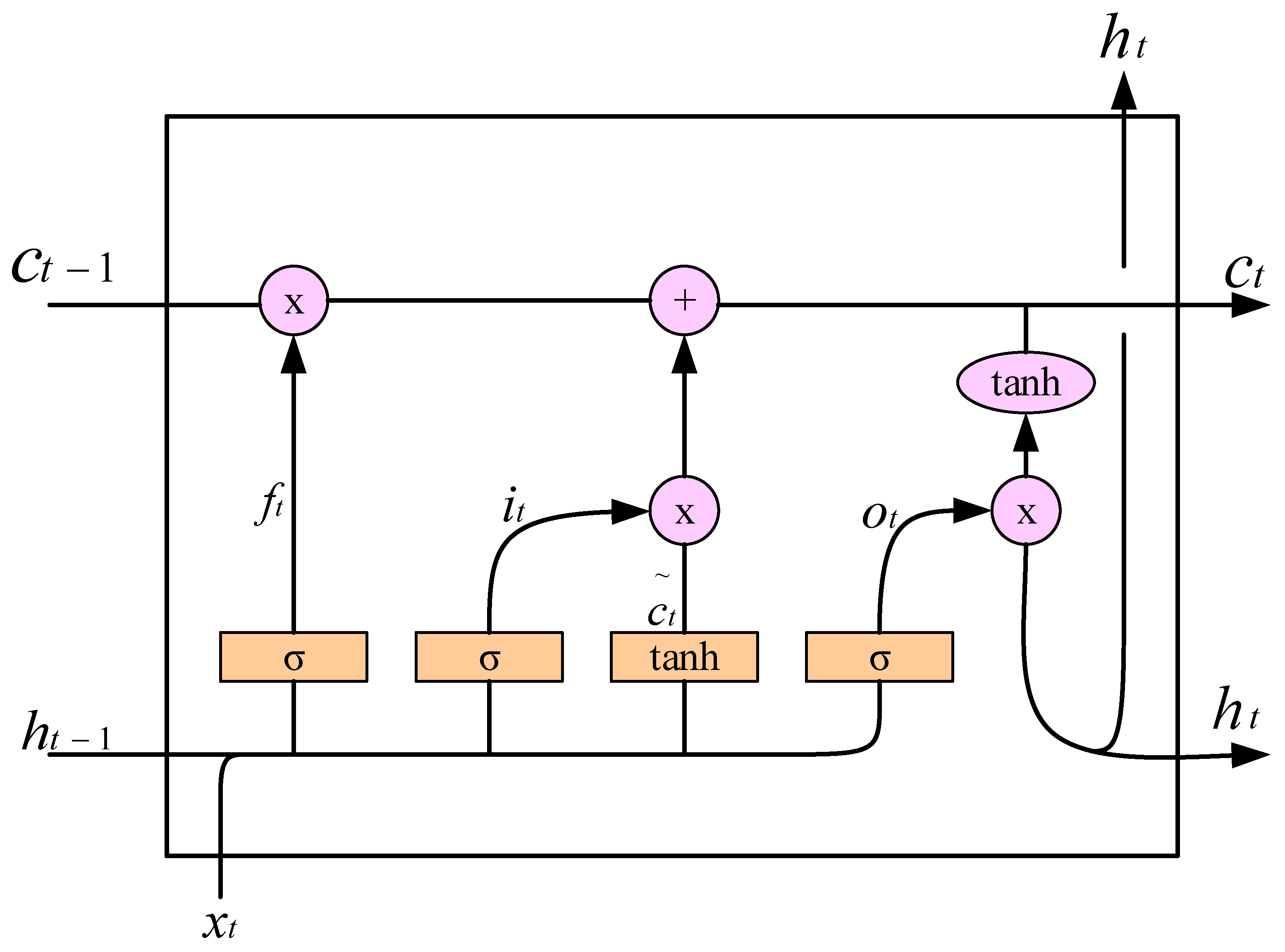
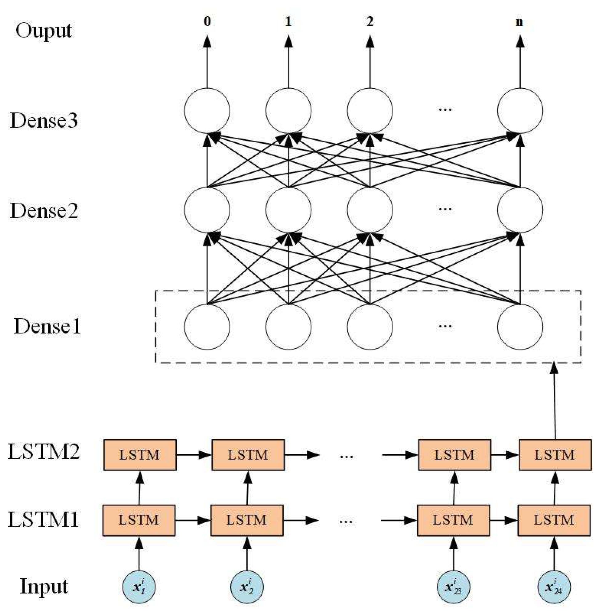
2.1. Long Short-Term Memory

The long Short-Term Memory network is a special kind of recurrent neural network (RNN) [30]. The network model can solve the disadvantages of the RNN, i.e., the gradient vanishing and the long-term dependency problem [31]. LSTM proposes a gating mechanism, including the forget gate, input gate and output gate. With these three basic gates, LSTM only remembers information that needs to be remembered for a long time and forgets short-term and unimportant information. The basic unit structure of the LSTM network is shown in Figure 1.

Figure 1. The basic unit structure of the LSTM network. Where “×” and “+” represent the matrix multiplication and matrix addition, respectively. σ is the sigmoid activation function and $\tanh$ is the tanh activation function. $f_t$ is the forget gate, $i_t$ is the input gate, $O_t$ is the output gate, $h_{t-1}$ and $h_t$ are the hidden states, $x_t$ denotes the input and $C_{t-1}$ and $C_t$ are the cell states. As can be seen from Figure 1, LSTM has three gates, namely, the forget gate $f_t$, input gate $i_t$ and output gate $O_t$. The forget gate $f_t$ reads the information of the state of the previous moment $h_{t-1}$ and the current state information $x_t$. The forget gate $f_t$ outputs a value between 0 and 1 from the previous cell via the sigmoid activation function σ. If the result is 0, the information of the previous unit is completely forgotten. In addition, the information of the previous unit is completely remembered.

The sigmoid activation function [32] takes any real value as the input and output values in the range of 0 to 1, which are then used in the LSTM to process the input values. The sigmoid function is used to convert the input to [0, 1] and to obtain the degree of forget $f_t$, as shown in Formula (1):

$$f_t=\sigma (W_f\cdot [h_{t-1},x_t]+b_f),$$

(1)

where $W_f$ is the weight coefficient matrix and $b_f$ is the bias matrix.

After the data pass through the forget gate, the input gate $i_t$ determines how much input information $x_t$ to store in the current cell.

Firstly, the input gate $i_t$ selects the information $x_t$ to update through the sigmoid activation function σ, as shown in Formula (2):

$$i_t=\sigma (W_i\cdot [h_{t-1},x_t]+b_i),$$

(2)

where $b_i$ is the bias matrix and $W_i$ is the weight coefficient matrix.

Then, using tanh activation function $\mathrm{Tanh}$, the selected information is processed to generate an alternative update vector ${\tilde{C}}_t$, as shown in Formula (3):

$${\tilde{C}}_t=\tanh (W_C\cdot [h_{t-1},x_t]+b_C),$$

(3)

where $W_C$ is the weight coefficient matrix and $b_C$ is the bias matrix.

In addition, the above two steps can be combined to update the status of the current unit and update the previous status information $C_{t-1}$. We let the previous status information $C_{t-1}$ be multiplied by the degree of forget $f_t$, which stands for the forgotten part. Then, we could add the forgotten part and the product of the input gate information $i_t$, as well as the alternative update vector ${\tilde{C}}_t$, as shown in Formula (4):

$$C_t=f_t*C_{t-1}+i_t*{\tilde{C}}_t,$$

(4)

Finally, we let the output of the previous cell $h_{t-1}$ and the input $x_t$ determine which information to output with the sigmoid activation function σ and which multiplied information was output, as well as the cell state, handled with the use of the tanh activation function tanh, as shown in Formulas (5) and (6):

$$o_t=\sigma (W_o\cdot [h_{t-1},x_t]+b_o),$$

(5)

$$h_t=o_t*\tanh (C_t),$$

(6)

where $W_o$ is the weight coefficient matrix and $b_o$ is the bias matrix.

2.2. Hunter–Prey Optimization Algorithm

The hunter–prey optimization (HPO) algorithm is a new optimization algorithm used to solve optimization problems [33,34,35]. The algorithm was inspired by the hunting behavior of some carnivores, such as lions, tigers and leopards, as well as prey, such as deer and antelopes [36,37]. In the proposed method, hunters usually give priority to the prey far away from its group. The hunter adjusts its position towards the prey far away from its group whilst the prey adjusts its position towards the group. The search agent’s position is considered as a safe place through the optimum value of the fitness function.

The steps of the hunter–prey optimizer are as follows:

Firstly, same as most optimization algorithm structures, in each iteration, the position of each hunter and prey is updated according to the rules of the algorithm, and the new position of each member is re-evaluated using the objective function. The position of each member in the initial group is randomly generated in the search space, as shown in Formula (7):

$$x_i=rand(1,d)\times (ub-lb)+lb,$$

(7)

where $x_i$ is the hunter’s position, $lb$ is the minimum for the problem variables, $ub$ is the maximum value for the problem variables and d is the number of variables of the problem.

Secondly, the search mechanism of the hunter generally involves two steps: exploration and exploitation. Exploration is the tendency of hunters to search in a highly random manner to find the regions of more likely prey. After promising regions are found, exploitation is applied, which is when a hunter must reduce random behavior in order to search for prey around a promising area. The search mechanism of a hunter is shown in Formula (8):

$$x(t+1)=x(t)+\frac{[(2CZ{P}_{pos}-x(t))+(2(1-C)Z\mu -x(t)]}{2},$$

(8)

where $x(t)$ is the hunter’s current position, $x(t+1)$ is the hunter’s next position, $P_{pos}$ is the prey’s position, $\mu$ is the mean of all the positions, C is the balance parameter between exploration and exploitation, its value decreasing from 1 to 0.02 during the iteration, as shown in Formula (9), and Z is an adaptive parameter, as shown in Formula (10):

$$C=1-it(\frac{1-0.98}{MaxIt}),$$

(9)

$$Z=\overrightarrow{R_1}\otimes idx+\overrightarrow{R_2}\otimes (\sim idx),$$

(10)

where $it$ is the number of the current iteration and $MaxIt$ is the maximum number of iterations, the value of which in this study was set to 100. $\overrightarrow{R_1}$ and $\overrightarrow{R_2}$ are random vectors in the range [0, 1] and $idx$ is the index number of the vector that satisfies the condition $\overrightarrow{R_1}<C$.

Then, according to the hunting scenario, when the hunter takes the prey, it dies, and the next time, the hunter moves to the location of the dead prey. The iteration can be continued with the prey’s position being the new hunter position. In addition, assuming that the best safe location is the best global location, since it gives the prey a better chance of survival, the hunter may choose another prey, as shown in Formula (11):

$$x(t+1)={\mathrm{T}}_{pos}+CZ\cos (2\pi R_3)\times ({\mathrm{T}}_{pos}-x(t)),$$

(11)

where $x(t)$ is the hunter’s current position, $x(t+1)$ is the hunter’s next position, $T_{pos}$ is the global optimal position that has the best fitness from the first iteration to the current iteration and $R_3$ is a random number in the range [−1, 1].

Finally, it is important how the hunter and prey are chosen in this algorithm, as shown in Formula (12):

$$x(t+1)=\left\{\begin{array}{l}x(t)+0.5[(2CZ{P}_{pos}-x(t))+(2(1-C)Z\mu -x(t)]{\hspace{1em}\hspace{1em}\hspace{1em}\mathrm{R}}_4<\beta \\ {\mathrm{T}}_{pos}+CZ\cos (2\pi R_3)\times ({\mathrm{T}}_{pos}-x(t)){\hspace{1em}\hspace{1em}\hspace{1em}\hspace{1em}\hspace{1em}\hspace{1em}\hspace{1em}\hspace{1em} \mathrm{R}}_4\ge \beta \end{array}\right.,$$

(12)

where R₄ is a random number in the range [0, 1] and $\beta$ is an adjusting parameter, whose value in this study was set to 0.15.

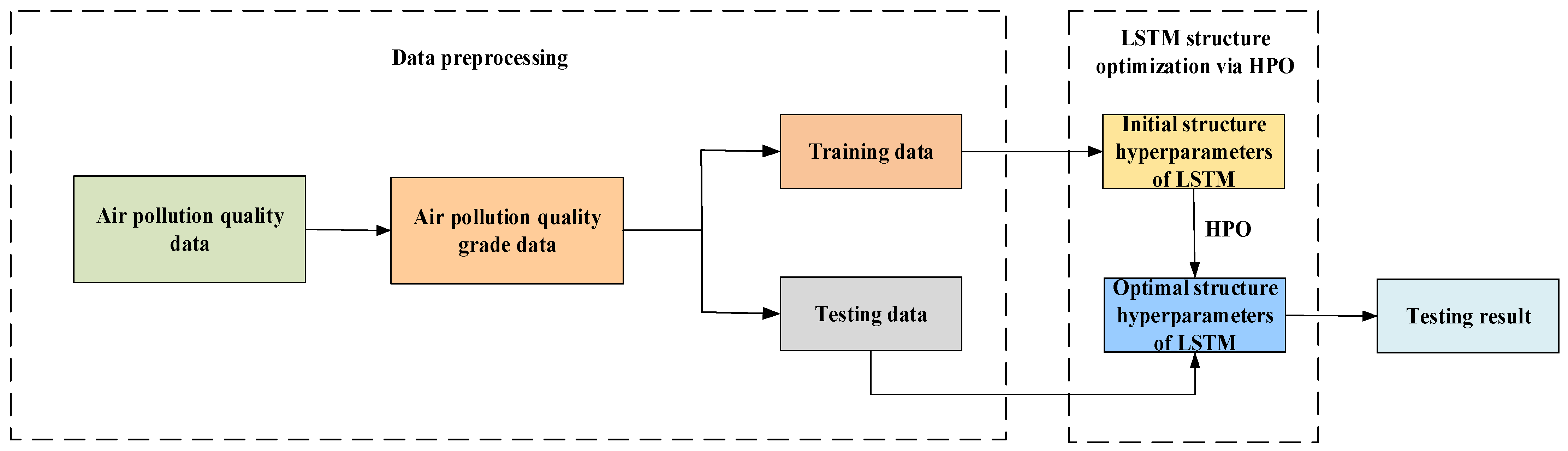
3. The Proposed Method

This section introduces the data preprocessing conducted before the air quality grade prediction based on the LSTM network. We also represented the hunter–prey optimization algorithm to optimize a more powerful LSTM network structure. The proposed method includes the three major steps: (1) data preprocessing, that is the air quality data are disposed of as grade data; (2) the hunter–prey optimization algorithm that determines the optimal hyperparameter of the LSTM network structure; and (3) the LSTM network via the optimization of the hyperparameters employed for the training and testing of grade data. The flowchart of the proposed method is shown in Figure 2.

Figure 2. The flowchart of the proposed method.

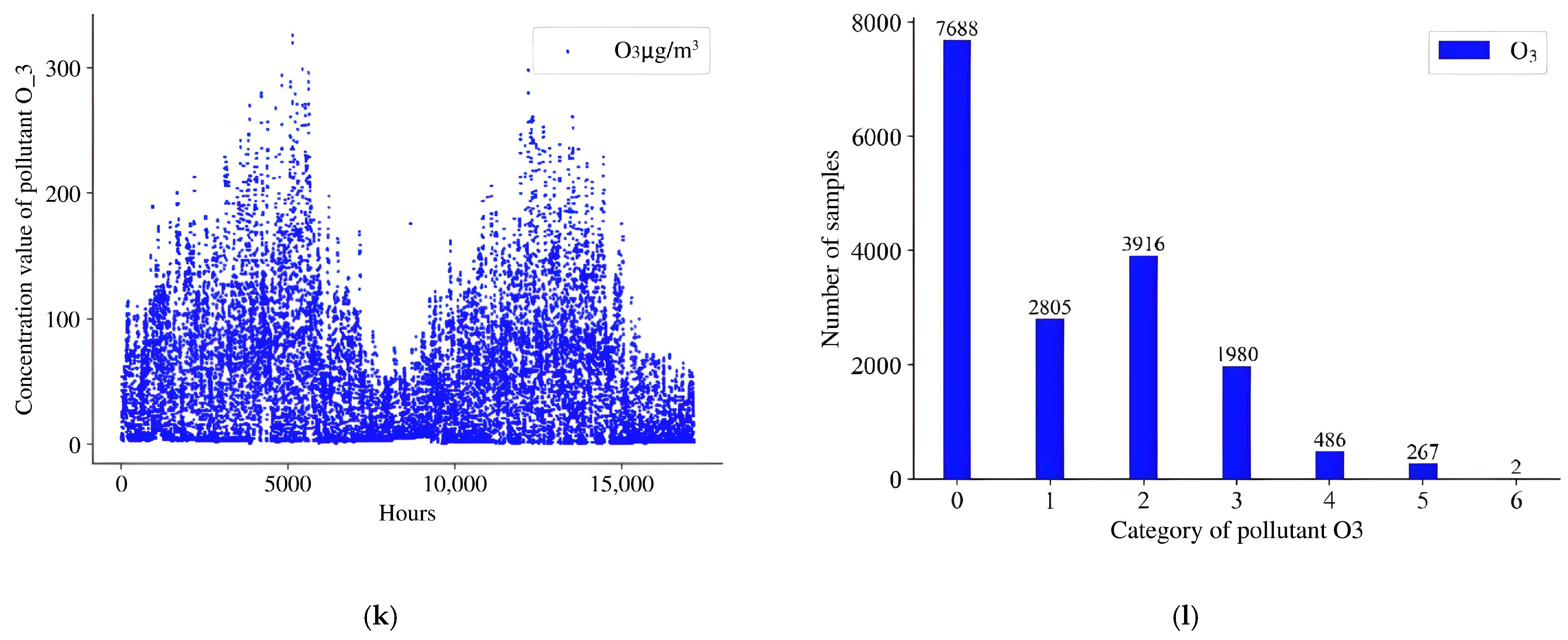
3.1. Data Preprocessing

To demonstrate the data preprocessing process, we took the real-time reported air quality index 2018–2020 data recorded at the Central Square Station of the Xin Cheng district, Xi’an city, as the sample. The average hourly concentrations of fine particulate matter (PM_2.5), inhalable particulate matter (PM₁₀), sulfur dioxide (SO₂), nitrogen dioxide (NO₂), carbon monoxide (CO) and ozone (O₃) in 2018–2020 were selected to be included in the original dataset. Dataset examples are shown in Table 1.

Table 1. Three-hour examples of air pollutant data from the Central Square Station of the Xi’an Xin Cheng district in Xi’an city from 2018 to 2020.

Time	PM10 (μg/m3)	PM2.5 (μg/m3)	SO2 (μg/m3)	NO2 (μg/m3)	CO (μg/m3)	O3 (μg/m3)
2018-01-01 01:00	436	201	27	85	2.2	5
2018-01-01 02:00	403	261	24	77	2.5	6
2018-01-01 03:00	477	358	33	79	2.9	7

We divided the concentration of air pollutants in the original dataset into the corresponding pollutant quality grade. This method not only achieved the prediction of air pollution quality, but also transformed the problem of data fitting into a problem of data classification, simplifying the difficulty of the problem and displaying the forecast results visually. The partitions of air pollution quality grades are shown in Table 2.

Table 2. The partitions of air pollution quality grades.

Grade	PM10 (μg/m3)	PM2.5 (μg/m3)	SO2 (μg/m3)	NO2 (μg/m3)	CO (μg/m3)	O3 (μg/m3)
0	0–50	0–35	0–150	0–100	0–5	0–160
1	51–150	35–75	150–500	100–200	5–10	160–200
2	150–250	75–115	500–650	200–700	10–35	200–300
3	250–350	115–150	650–800	700–1200	35–60	300–400
4	350–420	150–250	800+	1200–2340	60–90	400–800
5	420–500	250–350	-	2340–3090	90–120	800–1000
6	500–600	350–500	-	3090–3840	120–150	1000–1200
7	600+	500+	-	3840+	150+	1200+

Compared with Table 1, the quality grades of the air pollutant data examples at the Central Square Station of the Xi’an Xin Cheng district in Xi’an city after Conversion are shown in Table 3.

Table 3. An example of air pollutant grades at the Central Square Station of Xi’an Xin Cheng district in Xi’an city from 2018 to 2020.

Time	PM10 Grades	PM2.5 Grades	SO2 Grades	NO2 Grades	CO Grades	O3 Grades
2018-01-01 01:00	5	4	0	0	0	0
2018-01-01 02:00	4	5	0	0	0	0
2018-01-01 03:00	5	6	0	0	0	0

After classifying the concentration value interval of air pollutants according to Table 3, some classified pollutant quality grade data were concentrated in grade 0. To solve this problem, we redivided the pollutant concentration intervals into corresponding pollutant quality grades based on Table 2, according to the data distribution of pollutants whose concentration values were concentrated in category 0, as shown in Table 4.

Table 4. Air pollutant concentration value interval division after redivision.

Grade	PM10 (μg/m3)	PM2.5 (μg/m3)	SO2 (μg/m3)	NO2 (μg/m3)	CO (μg/m3)	O3 (μg/m3)
0	0–50	0–35	0–5	0–30	0–0.6	0–25
1	50–150	35–75	5–10	30–50	0.6–1.0	25–50
2	150–250	75–115	10–15	50–100	1.0–1.5	50–100
3	250–350	115–150	15–150	100–200	1.5–5	100–160
4	350–420	150–250	150–500	200–700	-	160–200
5	420–500	250–350	-	-	-	200–300
6	500–600	350–500	-	-	-	300–400
7	600+	-	-	-	-	-

After the second division classifying the concentration value interval of the air pollutants, according to Table 4, an example of air pollutant grades at the Central Square Station of Xi’an Xin Cheng district in Xi’an city from 2018 to 2020 is shown in Table 5.

Table 5. An example of air pollutant grades at the Central Square Station of the Xi’an Xin Cheng district in Xi’an city from 2018 to 2020 after redivision classification.

Time	PM10 Grades	PM2.5 Grades	SO2 Grades	NO2 Grades	CO Grades	O3 Grades
2018-01-01 01:00	5	4	3	2	3	0
2018-01-01 02:00	4	5	3	2	3	0
2018-01-01 03:00	5	6	3	2	3	0

After the second division classifying the concentration value of air pollutants, according to Table 4, Figure 3 shows the distribution of air quality grade data and the number of data contained in the corresponding category.

Figure 3. Scatter plots of pollutant concentrations and bar charts of each grade of air pollution. (a,b): PM₁₀; (c,d): PM_2.5; (e,f): SO₂; (g,h): NO₂; (i,j): CO; (k,l): O₃.

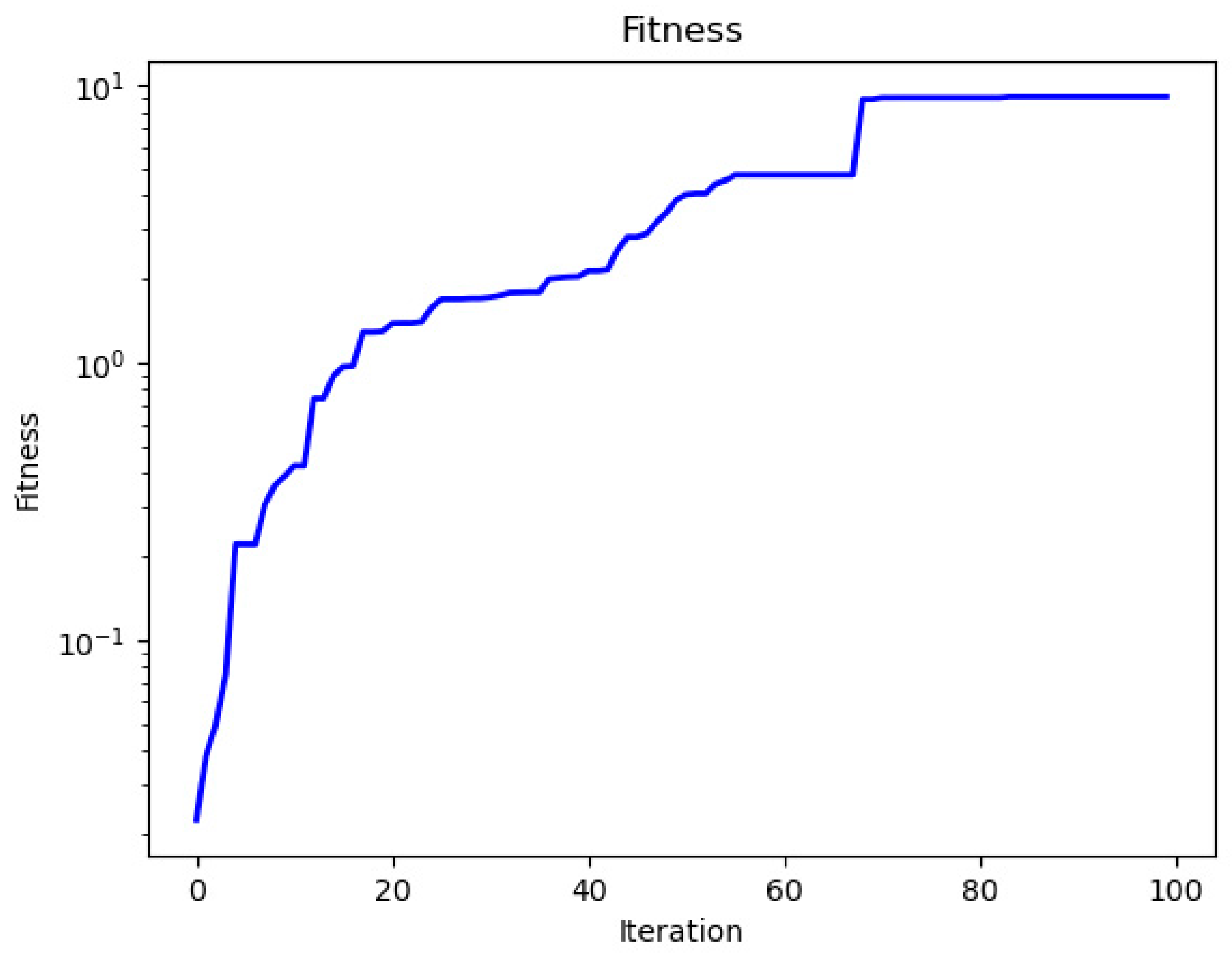
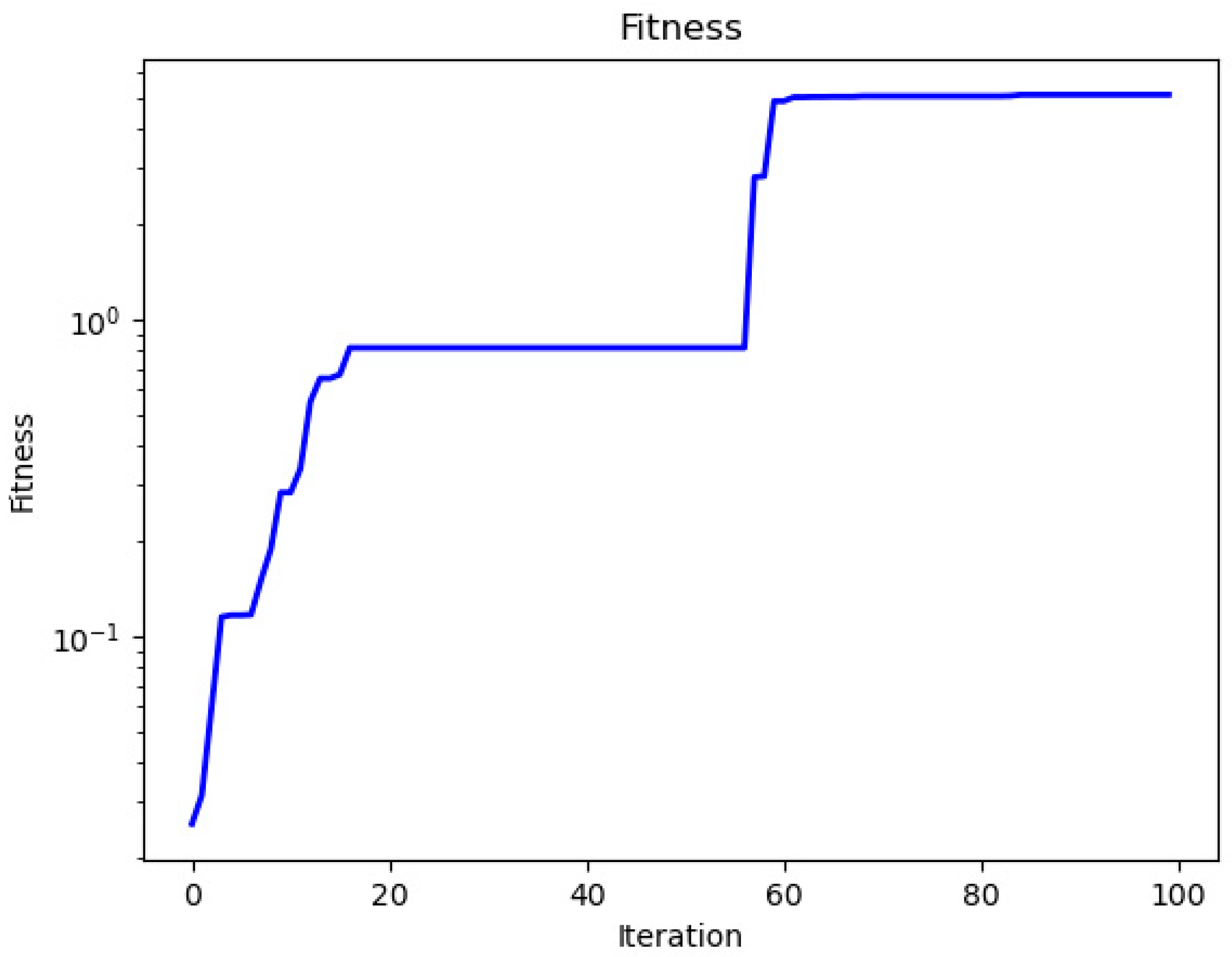
3.2. The Network Hyperparameters of LSTM Optimized via HPO Algorithm

In this paper, according to the air quality monitoring station, we used air pollutant quality grade data $(x_1^i,x_2^i,\dots ,x_h^i)$ in the first $h$ hours to predict the air pollutant quality level data $x_{h+1}^i$ in $h+1$ hour. The formula used was Formula (13):

$$x_{h+1}^i=f((x_1^i,x_2^i,\dots ,x_h^i)),$$

(13)

where $f$ is the mapping function. The LSTM network model is shown in Figure 4.

Figure 4. The LSTM neural network model.

We designed six hyperparameters of the LSTM network to determine the predictions because there were six types of air pollutants. The LSTM network model is shown in Figure 5. Here, $x_{24}^i$ is the input of the LSTM network, 24 is the serial amount of data of one air pollutant in 24 h and the n-th element of the X denotes $n$ as the output of the network. LSTM1 and LSTM2 are the LSTM network cell layers; Dense1, Dense2 and Dense3 are the fully connected layers. Meanwhile, we also designed the hyperparameters of the LSTM structure, i.e., the number of layers of the LSTM network $a_0$, the number of LSTM units $a_1$, the number of fully connected layers $a_2$, the number of fully connected units $a_3$, the batch size $a_4$, the value of dropouts $a_5$ and the value of recurrent dropouts $a_6$.

Figure 5. The iteration and corresponding fitness on dataset 1.

Then, we used the hunter–prey optimization algorithm to optimize the LSTM network to obtain the optimized network structure via optimizing the hyperparameters. The process of the specific algorithm model was as follows:

Firstly, we built the hunter–prey optimization algorithm model and initialized the algorithm, including initializing the adjusting parameter $\beta$ and setting the maximum number of iterations $MaxIt$.

Secondly, we used the list $[a_0,a_1,a_2,a_3,a_4,a_5,a_6]$ as the input for the HPO algorithm. We then calculated the fitness, recorded the global optimality $T_{pos}$ and updated the adaptive parameter Z.

Thirdly, the predator or prey locations were updated using Formula (12), after which we recalculated the fitness and current optimal value $P_{pos}$.

Then, the hunter–prey optimizer model looped to the maximum number of iterations and obtained the optimal solution $[a_0{}^{\prime },a_1{}^{\prime },a_2{}^{\prime },a_3{}^{\prime },a_4{}^{\prime },a_5{}^{\prime },a_6{}^{\prime }]$ as the new LSTM network hyperparameters. The process for the hyperparameters of the LSTM network structure optimized using the HPO algorithm is shown in Algorithm 1.

Finally, we used the new LSTM network adapted to the new network hyperparameters for training and testing.

Algorithm 1: The process for the hyperparameters of the LSTM network structure optimized using the HPO algorithm.

1: Input: The number of layers of the LSTM network $a_0$, the number of LSTM units $a_1$, the number of fully connected layers $a_2$, the number of fully connected units $a_3$, the batch size $a_4$, the value of dropouts $a_5$ and the value of recurrent dropouts $a_6$; 2: Initialization: Adjusting parameter $\beta$, the maximum number of iterations $MaxIt$ and the global optimal value $T_{pos}$; 3: For t = 1, 2, 3, …, T do 4: If range parameter < $\beta$, update the predator or prey location according to Formula (8); 5: If range parameter $\ge$$\beta$, update the predator or prey location according to Formula (11); 6: Calculating the fitness and the current optimal value $P_{pos}$; 7: Updating the adaptive parameter Z; 8: End for; 9: Output: The final optimal solution. $[a_0{}^{\prime },a_1{}^{\prime },a_2{}^{\prime },a_3{}^{\prime },a_4{}^{\prime },a_5{}^{\prime },a_6{}^{\prime }]$.

3.3. Training and Testing

For each dataset, the LSTM network was implemented in the training set corresponding with the dataset. In the process of the LSTM network, we set the number of iterations as 100, and the input was 24 h for the air quality grade. Next, the hunter–prey optimization algorithm was used to optimize the hyperparameters of the LSTM network. Finally, we obtained an air pollutant grade prediction method based on the LSTM network’s structure optimized via the hunter–prey optimization algorithm, i.e., the LSTM structure had the best hyperparameters in all individuals.

In this experiment, we used network structures to train datasets of air quality grade to obtain the final optimal predicted results. The network after 100 training iterations was obtained via the training set, and the predicted results were obtained by inputting the testing data.

4. Experiments and Analysis

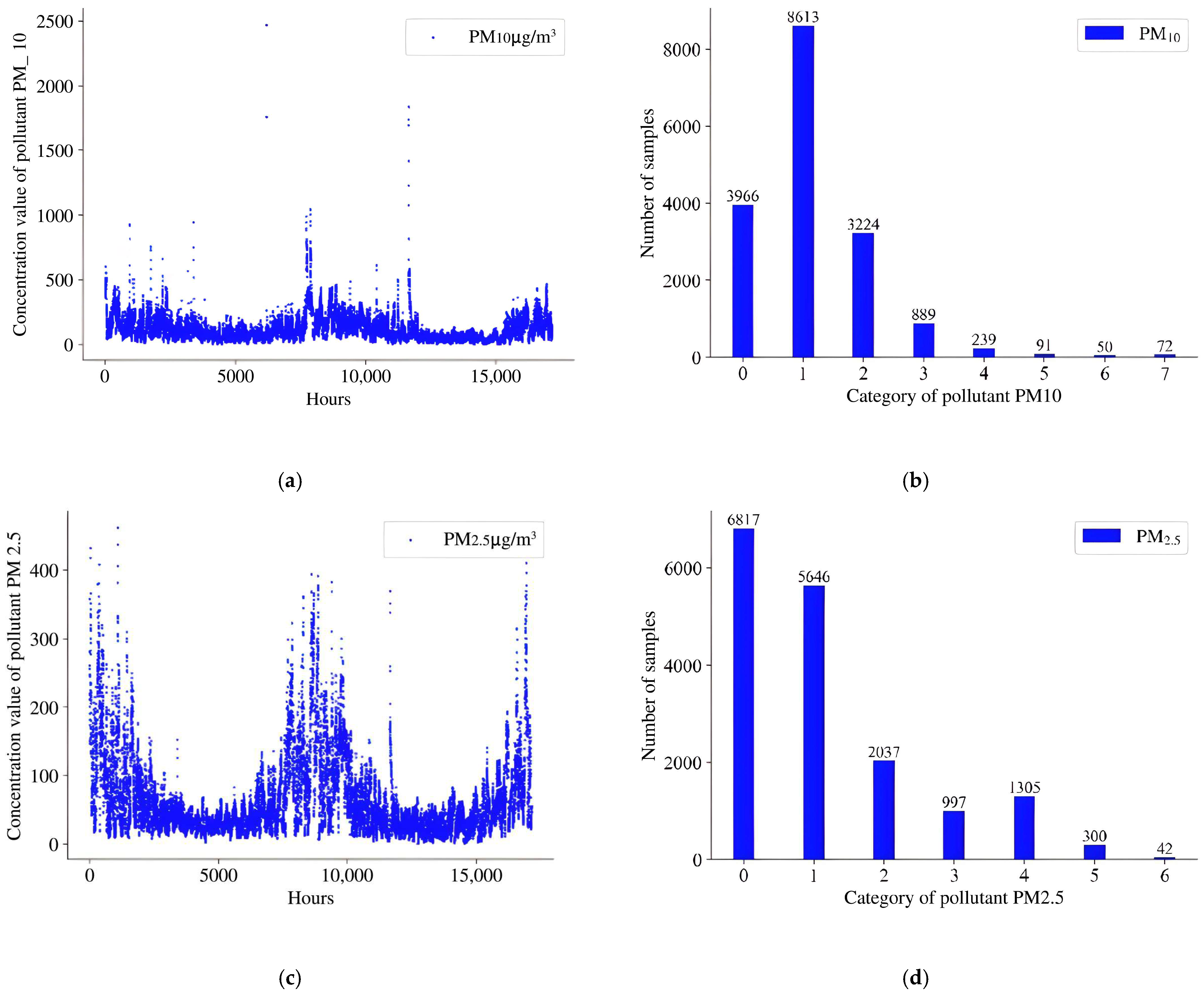
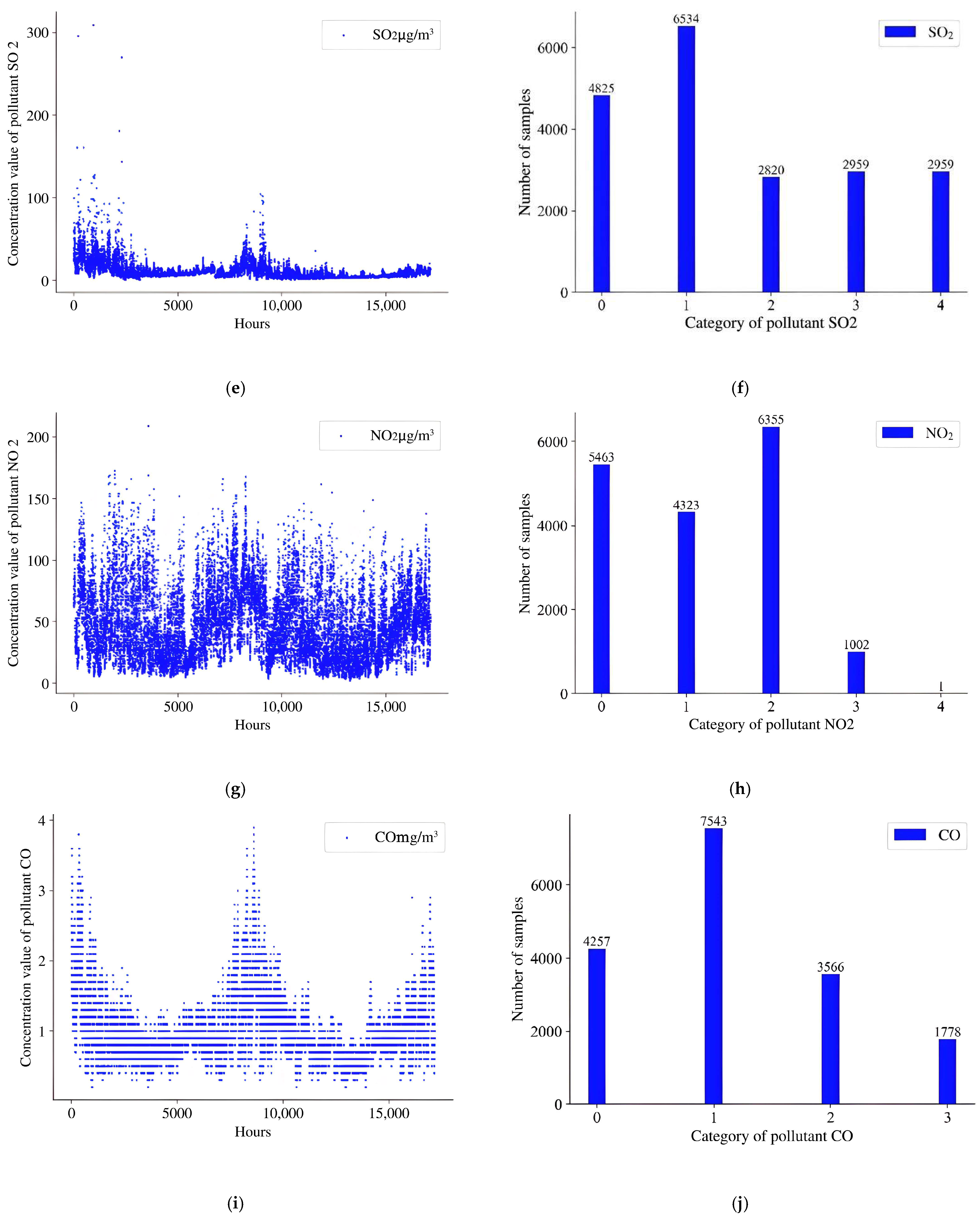
In order to verify the validity of the air pollutant grade prediction based on the LSTM network structure optimized with the use of the hunter–prey optimization algorithm, the actual data of three observation stations in Xi’an city were used for the experiments. The datasets, the experimental environment, experimental results and analyses used for the experiments are described below.

4.1. Datasets

In this paper, real-time air quality information collected at three air quality observation stations in Xi’an city was shown as the original dataset. We obtained the experimental dataset after grading all the data, as shown in Table 4. Dataset one: air quality data from the Central Station in Xi’an Xin Cheng Square from 2018 to 2020; dataset two: Xi’an Cao Tang Base air quality data; dataset three: Xi’an Gao Xin West Station air quality data.

The air quality dataset from the Xi’an Xin Cheng Center Square Station from 2018 to 2020 included 25,545 pieces of data; the Xi’an Cao Tang Base included 14,543 pieces of data; the Xi’an Gao Xin West Station had 14,544 pieces of data. These datasets were turned into reconstructed datasets after removing duplicates, outliers and null values. The reconstructed datasets from the Xi’an Xin Cheng Center Square Station from 2018 to 2020 included 25,064 pieces of data; the Xi’an Cao Tang Base included 14,321 pieces of data; the Xi’an Gao Xin West Station had 13,711 pieces of data. The quantity of data in the three datasets are shown in Table 6.

Table 6. The quantity of data in three datasets.

Dataset Name	Xin Cheng Center Square Station	Cao Tang Base	Gao Xin West Station
Number	Dataset 1	Dataset 2	Dataset 3
Original Datasets	25,545	14,543	14,544
Reconstructed Datasets	25,064	14,321	13,711

In this paper, every 25 consecutive hours of data were considered a sample. The input data were the data of the first 24 h in the data of 25 consecutive hours, and the data of the last 1 h were considered the target.

In addition, dataset one for 2018 and 2019 was used as the training set and dataset one for 2020 was used as the testing set. Both dataset two and dataset three were divided into the training and testing sets using a ratio of 1:1.

The training set and testing set numbers divided from each reconstructed dataset are shown in Table 7.

Table 7. The number of samples in the training set and testing set of three datasets.

Dataset	Number of Samples
	Training Set	Testing Set
Dataset 1	17,120	7896
Dataset 2	6976	6976
Dataset 3	6476	6476

4.2. The Experimental Environment

The number of iterations for the LSTM was set to 100. The learning rate is a tuning parameter in back propagation that determines the step size at each iteration while moving toward the minimum of a loss function. In this experiment, the learning rate was set to 0.02. The number of LSTM network layers, the number of LSTM units, the number of fully connected layers, the number of fully connected units, the batch size, the value of dropouts and the value of recurrent dropouts were random.

4.3. The Experimental Evaluation Index

In order to evaluate the effectiveness of the air quality grade prediction model proposed in this paper, we calculated the accuracy by comparing the predicted category with the true category. The calculation of accuracy is shown in Formula (14):

$$accuracy=\frac{TP+TN}{TP+TN+FP+FN}\times 100\%,$$

(14)

where TN, FN, TP and FP are the true negative, false negative, true positive and false positive, respectively.

4.4. The LSTM Network

In order to prove the efficiency of the LSTM network used in this paper, we, respectively, applied the LSTM network in three datasets.

To prove the effectiveness of the LSTM network, we compared it with another two traditional network structures in three datasets. The details for the comparison of the structures for the three different networks were as follows:

BP: Included six fully connected layers;

RNN: Included three features in the hidden state and three hidden layers;

LSTM: Included three features in the hidden state and three hidden layers.

The accuracies of dataset one are shown in Table 8.

Table 8. The accuracies of LSTM network compared with traditional networks in dataset 1.

Methods	PM10	PM2.5	SO2	NO2	CO	O3
BP	84.3%	89.9%	72.8%	76.4%	74.9%	66.2%
RNN	84.6%	88.8%	85.5%	81.6%	83.7%	82.0%
LSTM	87.2%	90.0%	88.5%	83.2%	85.7%	83.3%

As shown in Table 9, the LSTM network structure obtained the best prediction results for all air pollutants. Especially in the prediction of the PM10 and SO₂ pollutant quality levels, the long short-term memory network method outperformed the next-best recurrent neural network method by nearly 3%.

Table 9. The accuracies of LSTM network compared with traditional networks in dataset 2.

Methods	PM10	PM2.5	SO2	NO2	CO	O3
BP	85.2%	90.8%	75.0%	82.2%	82.3%	78.3%
RNN	81.2%	87.2%	71.2%	79.3%	82.2%	74.6%
LSTM	86.2%	91.3%	83.9%	83.8%	86.0%	83.2%

The accuracies of dataset two are shown in Table 9.

As shown in Table 10, the accuracies obtained in the air quality grade prediction of six pollutants were the best in dataset two, whose PM₁₀, PM_2.5, SO₂, NO₂, CO and O₃ were 86.2%, 91.3%, 83.9%, 83.8%, 86.0% and 83.2%, respectively. Especially in the prediction of the sulfur dioxide (SO₂) pollutant quality level, the accuracy of the LSTM method was 9% higher than that of the BP neural network method.

Table 10. The accuracies of LSTM network compared with traditional networks in dataset 3.

Methods	PM10	PM2.5	SO2	NO2	CO	O3
BP	87.2%	77.7%	84.4%	81.0%	81.0%	84.2%
RNN	84.4%	77.6%	70.3%	78.3%	72.3%	84.5%
LSTM	86.9%	85.6%	85.2%	82.9%	83.3%	85.1%

The results of dataset three are shown in Table 10.

As shown in Table 11, the LSTM network structure obtained the best prediction results for five kinds of air pollutants. In PM₁₀, the LSTM achieved the second best predicted accuracy, which was almost equal to the best one.

Table 11. The variations of fitness and corresponding network hyperparameters in dataset 1.

Iterations	Fitness	Network Hyperparameters
00	0.019	{1, 24, 2, 6, 128, 0.1, 0.1}
01	0.073	{1, 24, 2, 6, 128, 0.1, 0.1}
03	0.096	{1, 24, 2, 6, 128, 0.1, 0.1}
05	0.102	{1, 24, 2, 6, 128, 0.1, 0.1}
10	0.548	{2, 24, 2, 6, 128, 0.1, 0.1}
20	0.955	{3, 24, 2, 6, 128, 0.1, 0.2}
30	1.312	{3, 24, 3, 6, 128, 0.1, 0.3}
50	4.823	{3, 24, 3, 12, 128, 0.12, 0.3}
80	9.753	{3, 24, 3, 12, 128, 0.15, 0.3}
100	9.753	{3, 24, 3, 12, 128, 0.15, 0.3}

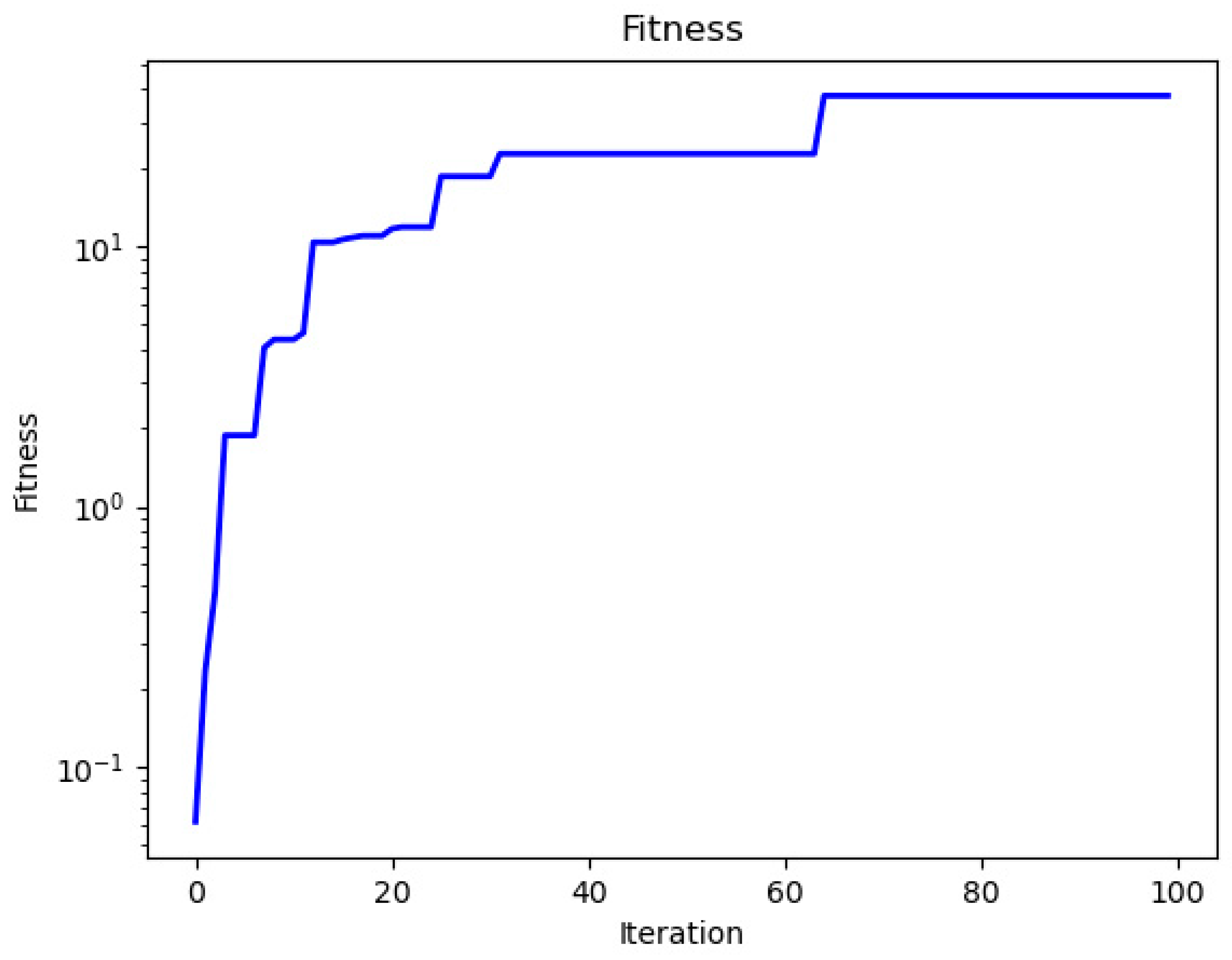
4.5. The LSTM Optimized via Hunter–Prey Optimization Algorithm

In order to prove the effectiveness of the hunter–prey optimization algorithm in optimizing the LSTM network, we, respectively, applied the hunter–prey optimization algorithm to process the LSTM network structure in three datasets. The bigger fitness showed that the LSTM network structure was better.

The iteration and corresponding best fitness of dataset one are shown in Figure 5.

The fitness and corresponding network hyperparameters at each iteration are shown in Table 11.

The iteration and corresponding fitness of dataset two are shown in Figure 6.

Figure 6. The iteration and corresponding fitness in dataset 2.

The fitness and corresponding network hyperparameter at each iteration are shown in Table 12.

Table 12. The variations of fitness and corresponding network hyperparameters in dataset 2.

Iterations	Fitness	Network Hyperparameters
00	0.026	{1, 24, 2, 6, 128, 0.1, 0.1}
01	0.035	{1, 24, 2, 6, 128, 0.1, 0.1}
03	0.059	{1, 24, 2, 6, 128, 0.1, 0.1}
05	0.082	{1, 24, 2, 6, 128, 0.1, 0.1}
10	0.211	{2, 24, 2, 6, 128, 0.1, 0.1}
20	0.929	{3, 24, 2, 6, 128, 0.1, 0.1}
30	0.929	{3, 24, 2, 6, 128, 0.1, 0.1}
50	0.929	{3, 24, 2, 6, 128, 0.1, 0.1}
80	8.675	{3, 24, 3, 16, 128, 0.2, 0.25}
100	8.675	{3, 24, 3, 16, 128, 0.2, 0.25}

The iteration and corresponding fitness of dataset three are shown in Figure 7.

Figure 7. The iteration and corresponding fitness in dataset 3.

The fitness and corresponding network hyperparameters at each iteration are shown in Table 13.

Table 13. The best fitness and corresponding network hyperparameters in dataset 3.

Iterations	Fitness	Network Hyperparameters
00	0.047	{1, 24, 2, 6, 128, 0.1, 0.1}
01	0.083	{1, 24, 2, 6, 128, 0.1, 0.1}
03	0.356	{1, 24, 2, 6, 128, 0.1, 0.1}
05	0.643	{1, 24, 2, 6, 128, 0.1, 0.1}
10	2.711	{2, 24, 2, 6, 128, 0.15, 0.2}
20	9.743	{3, 24, 3, 12, 128, 0.2, 0.2}
30	14.349	{3, 24, 3, 16, 128, 0.2, 0.35}
50	15.652	{3, 24, 3, 16, 128, 0.2, 0.3}
80	18.238	{3, 24, 3, 16, 128, 0.2, 0.35}
100	18.238	{3, 24, 3, 16, 128, 0.2, 0.35}

As shown in Figure 4, Figure 5 and Figure 6, we focused on the changes in the optimal fitness and corresponding iterations in detail.

As can be seen from Table 12, Table 13 and Table 14, the best fitness always appeared in the ultimate generation; therefore, the best network hyperparameters were in the last generation of the HPO algorithm.

Table 14. The accuracies of the LSTM_HPO compared with LSTM and LSTM_WOA in dataset 1.

Methods	PM10	PM2.5	SO2	NO2	CO	O3
LSTM	87.2%	90.0%	88.5%	83.2%	85.7%	83.3%
LSTM_WOA	89.0%	91.1%	90.3%	87.0%	86.8%	86.2%
LSTM_HPO	90.4%	91.7%	92.1%	88.9%	88.3%	87.7%

Finally, the optimal number of layers of the LSTM, the number of fully connected layers, the number of fully connected units, the dropouts and the recurrent dropouts in dataset one were 3, 3, 12, 0.15 and 0.3, respectively. The optimal number of layers of the LSTM, the number of fully connected layers, the number of fully connected units, the dropouts and the recurrent dropouts in dataset two were 3, 3, 16, 0.2 and 0.25, respectively. Additionally, the optimal number of layers of the LSTM, the number of fully connected layers, the number of fully connected units, the dropouts and the recurrent dropouts in dataset three were 3, 3, 16, 0.2 and 0.35, respectively.

4.6. The Proposed Method Compared with LSTM and LSTM Optimized via WOA

In this paper, the HPO algorithm was used to optimize the seven parameter dimensions of the LSTM network: the number of layers, the number of LSTM units, the number of fully connected layers, the number of fully connected units, the batch size, the value of dropouts and the value of recurrent dropouts.

To prove the effectiveness of these seven parameter dimensions via HPO algorithm, we compared the LSTM_HPO with the LSTM optimized via the whale optimization (LATM_WOA) algorithm and the LSTM. These three LSTM network structures were designed as follows:

LSTM: Three features in the hidden state, three hidden layers and three fully connected layers;

LSTM_WOA [38,39]: The LSTM optimized via the whale optimization algorithm;

LSTM_HPO: The LSTM optimized via the hunter–prey optimization algorithm.

The results in dataset one are shown in Table 14.

As shown in Table 14, the accuracy of the LSTM_HPO was higher than that of the LSTM and LSTM_WOA in predicting the quality grades of PM₁₀, PM_2.5, SO₂, NO₂, CO and O₃.

The results in dataset two are shown in Table 15.

Table 15. The accuracies of the LSTM_HPO compared with LSTM and LSTM_WOA in dataset 2.

Methods	PM10	PM2.5	SO2	NO2	CO	O3
LSTM	86.2%	91.3%	83.9%	83.8%	86.0%	83.2%
LSTM_WOA	89.6%	91.6%	87.0%	85.4%	87.1%	85.4%
LSTM_HPO	89.4%	92.2%	88.1%	86.9%	89.1%	86.4%

As shown in Table 15, the LSTM_HPO performed better than the other LSTM network structures in five air pollutants in dataset two. In PM₁₀, the LSTM_HPO obtained the second best prediction results, which was almost equal to the best one.

The accuracies in dataset three are shown in Table 16.

Table 16. The accuracies of the LSTM_HPO compared with LSTM and LSTM_WOA in dataset 3.

Methods	PM10	PM2.5	SO2	NO2	CO	O3
LSTM	86.9%	85.6%	85.2%	82.9%	83.3%	85.1%
LSTM_WOA	88.9%	89.5%	88.9%	83.2%	86.4%	86.9%
LSTM_HPO	90.1%	90.1%	89.0%	85.7%	87.3%	88.2%

As can be seen from Table 16, the LSTM_HPO achieved the best prediction results compared with the other two network structure in dataset three.

It was apparent that the LSTM network optimized via the hunter–prey optimization algorithm derived from the proposed method on the three datasets could perform better than the LSTM network structures for most air pollutants.

5. Discussion

In this article, the lead time in prediction refers to the duration between the execute prediction and the occurrence of the actual result, which is of great significance for the practical application of air quality prediction. The lead time can provide more sufficient time for the government and the public to conduct relevant countermeasures; thus, the lead time in prediction is worth discussing. We verified the influence of different lead times in prediction in three datasets. The results for 6 h are shown in Table 17, Table 18 and Table 19.

Table 17. The accuracies of the LSTM_HPO for 6 h in dataset 1.

Lead Time	PM10	PM2.5	SO2	NO2	CO	O3
First hour	90.4%	91.7%	92.1%	88.9%	88.3%	87.7%
Second hour	87.3%	89.1%	90.5%	86.3%	86.3%	86.6%
Third hour	84.7%	86.5%	88.2%	83.6%	83.2%	85.1%
Fourth hour	83.7%	84.3%	86.3%	79.1%	80.6%	84.2%
Fifth hour	81.9%	82.0%	83.9%	76.4%	75.0%	82.8%
Sixth hour	77.5%	80.1%	81.5%	73.8%	71.4%	81.3%

Table 18. The accuracies of the LSTM_HPO for 6 h in dataset 2.

Lead Time	PM10	PM2.5	SO2	NO2	CO	O3
First hour	89.4%	92.2%	88.1%	86.9%	89.1%	86.4%
Second hour	86.3%	90.4%	85.9%	84.2%	86.4%	84.7%
Third hour	83.7%	88.5%	83.2%	81.3%	83.5%	83.1%
Fourth hour	79.7%	86.7%	81.6%	78.6%	80.6%	80.8%
Fifth hour	76.9%	82.0%	78.4%	74.2%	77.4%	78.9%
Sixth hour	72.5%	79.5%	74.9%	71.0%	73.8%	76.3%

Table 19. The accuracies of the LSTM_HPO for 6 h in dataset 3.

Lead Time	PM10	PM2.5	SO2	NO2	CO	O3
First hour	90.1%	90.1%	89.0%	85.7%	87.3%	88.2%
Second hour	86.3%	88.3%	87.6%	82.2%	85.1%	86.7%
Third hour	83.8%	85.7%	85.6%	79.3%	82.5%	84.5%
Fourth hour	80.9%	82.4%	83.2%	76.9%	78.6%	82.3%
Fifth hour	77.5%	79.5%	80.8%	72.6%	73.4%	80.1%
Sixth hour	74.8%	77.4%	78.1%	69.7%	68.6%	77.9%

As we can see, it is apparent that the proposed method used on the three datasets could provide benefits in real-life applications. Additionally, a higher lead time led to a higher number of predicted faults, resulting in this phenomenon looking like weather prediction.

6. Conclusions

In this paper, we proposed an air pollutant quality grade prediction method based on the hyperparameter-optimization-inspired long short-term memory (LSTM) network. Firstly, the air quality data were transformed into grade data, which meant that the air quality data were partitioned into grades, i.e., we turned the fitting problem into a classification task. Secondly, we chose LSTM to address the task of obtaining an air quality grade prediction. Furthermore, the LSTM network hyperparameters optimized through the use of the hunter–prey optimization algorithm obtained better results. Compared with the other air quality grade prediction methods, our proposed method showed effective performance for the air quality grade prediction task in three datasets. Our method especially improved the accuracy by 4.1%, 4% and 3.8%, when predicting the air quality grade of SO₂, CO and O₃, respectively.

In future experiments, future studies can improve the accuracy of the results by increasing the amount of data and optimizing the performance of the model in terms of analyzing the influencing factors.

Due to the limitation of the detection range, differences in the level of urban development and the diversity of climatic conditions, our prediction results may not be applicable to air quality changes in other regions. Therefore, it is recommended to establish multiple air quality monitoring stations to monitor air quality and to lay a solid foundation for perfect air quality level predictions.

References

- Aliyu, Y.A.; Botai, J.O. Reviewing the local and global implications of air pollution trends in Zaria, northern Nigeria. Urban Clim. 2018, 26, 51–59. [Google Scholar] [CrossRef]
- Chen, Y.; Jiao, Z.; Chen, P.; Fan, L.; Zhou, X.; Pu, Y.; Du, W.; Yin, L. Short-term effect of fine particulate matter and ozone on non-accidental mortality and respiratory mortality in Lishui district, China. BMC Public Health 2021, 21, 1661. [Google Scholar] [CrossRef] [PubMed]
- Mądziel, M.; Campisi, T. Investigation of Vehicular Pollutant Emissions at 4-Arm Intersections for the Improvement of Integrated Actions in the Sustainable Urban Mobility Plans (SUMPs). Sustainability 2023, 15, 1860. [Google Scholar] [CrossRef]
- Jensen, S.S.; Ketzel, M.; Becker, T.; Christensen, J.; Brandt, J.; Plejdrup, M.; Winther, M.; Nielsen, O.-K.; Hertel, O.; Ellermann, T. High resolution multi-scale air quality modelling for all streets in Denmark. Transp. Res. Part D Transp. Environ. 2017, 52, 322–339. [Google Scholar] [CrossRef]
- Chauhan, A.J.; Johnston, S.L. Air pollution and infection in respiratory illness. Br. Med. Bull. 2003, 68, 95–112. [Google Scholar] [CrossRef] [PubMed]
- Plummer, L.E.; Smiley-Jewell, S.; Pinkerton, K.E. Impact of air pollution on lung inflammation and the role of Toll-like receptors. Int. J. Interferon Cytokine Mediat. Res. 2012, 4, 43–57. [Google Scholar]
- Cohen, A.J.; Brauer, M.; Burnett, R.; Anderson, H.R.; Frostad, J.; Estep, K.; Balakrishnan, K.; Dandona, L.; Dandona, R.; Feigin, V. Estimates and 25-year trends of the global burden of disease attributable to ambient air pollution: An analysis of data from the Global Burden of Diseases Study 2015. Lancet 2017, 389, 1907–1918. [Google Scholar] [CrossRef]
- Yin, P.; He, G.; Fan, M.; Chiu, K.Y.; Fan, M.; Liu, C.; Xue, A.; Liu, T.; Pan, Y.; Mu, Q.; et al. Particulate air pollution and mortality in 38 of China’s largest cities: Time series analysis. BMJ 2017, 356, j667. [Google Scholar] [CrossRef]
- Nations, U. The World’s Cities in 2018—Data Booklet; Department of Economic and Social Affairs: New York, NY, USA, 2018; Population Division. [Google Scholar]
- Alegria, A.; Barbera, R.; Boluda, R.; Errecalde, F.; Farré, R.; Lagarda, M.J. Environmental cadmium, lead and nickel contamination: Possible relationship between soil and vegetable content. Fresenius’ J. Anal. Chem. 1991, 339, 654–657. [Google Scholar] [CrossRef]
- Ercilla-Montserrat, M.; Muñoz, P.; Montero, J.I.; Gabarrell, X.; Rieradevall, J. A study on air quality and heavy metals content of urban food produced in a Mediterranean city (Barcelona). J. Clean. Prod. 2018, 195, 385–395. [Google Scholar] [CrossRef]
- Huang, M.; Zhang, T.; Wang, J.; Zhu, L. A new air quality forecasting model using data mining and artificial neural network. In Proceedings of the 6th IEEE International Conference on Software Engineering and Service Science (ICSESS), Beijing, China, 23–25 September 2015; pp. 259–262. [Google Scholar]
- Kang, G.K.; Gao, J.Z.; Chiao, S.; Lu, S.; Xie, G. Air quality prediction: Big data and machine learning approaches. Int. J. Environ. Sci. Dev 2018, 9, 8–16. [Google Scholar] [CrossRef]
- Afzali, A.; Rashid, M.; Afzali, M.; Younesi, V. Prediction of air pollutants concentrations from multiple sources using AERMOD coupled with WRF prognostic model. J. Clean. Prod. 2017, 166, 1216–1225. [Google Scholar] [CrossRef]
- Ghaemi, Z.; Farnaghi, M.; Alimohammadi, A. Hadoop-based distributed system for online prediction of air pollution based on support vector machine. Int. Arch. Photogramm. Remote Sens. Spat. Inf. Sci. 2015, 40, 215. [Google Scholar] [CrossRef]
- Wang, P.; Liu, Y.; Qin, Z.; Zhang, G. A novel hybrid forecasting model for PM10 and SO2 daily concentrations. Sci. Total Environ. 2015, 505, 1202–1212. [Google Scholar] [CrossRef]
- Rybarczyk, Y.; Zalakeviciute, R. Machine learning approaches for outdoor air quality modelling: A systematic review. Appl. Sci. 2018, 8, 2570. [Google Scholar] [CrossRef]
- Taghavifar, H.; Mardani, A.; Mohebbi, A.; Khalilarya, S.; Jafarmadar, S. Appraisal of artificial neural networks to the emission analysis and prediction of CO2, soot, and NOx of n-heptane fueled engine. J. Clean. Prod. 2016, 112, 1729–1739. [Google Scholar] [CrossRef]
- Taylan, O. Modelling and analysis of ozone concentration by artificial intelligent techniques for estimating air quality. Atmos. Environ. 2017, 150, 356–365. [Google Scholar] [CrossRef]
- Gao, M.; Yin, L.; Ning, J. Artificial neural network model for ozone concentration estimation and Monte Carlo analysis. Atmos. Environ. 2018, 184, 129–139. [Google Scholar] [CrossRef]
- García Nieto, P.J.; García-Gonzalo, E.; Bernardo Sánchez, A.; Rodríguez Miranda, A.A. Air quality modeling using the PSO-SVM-based approach, MLP neural network, and M5 model tree in the metropolitan area of Oviedo (Northern Spain). Environ. Model. Assess. 2018, 23, 229–247. [Google Scholar] [CrossRef]
- Gholizadeh, M.H.; Darand, M. Forecasting the Air Pollution with using Artificial Neural Networks: The Case Study; Tehran City. J. Appl. Sci. 2009, 9, 3882–3887. [Google Scholar] [CrossRef]
- Ai, H.; Shi, Y. Study on prediction of haze based on BP neural network. Comput. Simul. 2015, 32, 402–405 + 415. [Google Scholar]
- Zhao, W.; Xia, L.; Gao, G.; Cheng, L. PM2.5 prediction model based on weighted KNN-BP neural network. J. Environ. Eng. Technol. 2019, 9, 14–18. [Google Scholar]
- Biancofiore, F.; Busilacchio, M.; Verdecchia, M.; Tomassetti, B.; Aruffo, E.; Bianco, S.; Di Tommaso, S.; Colangeli, C.; Rosatelli, G.; Di Carlo, P. Recursive neural network model for analysis and forecast of PM10 and PM2.5. Atmos. Pollut. Res. 2017, 8, 652–659. [Google Scholar] [CrossRef]
- Liu, D.R.; Hsu, Y.K.; Chen, H.-Y.; Jau, H.-J. Air pollution prediction based on factory-aware attentional LSTM neural network. Computing 2021, 103, 75–98. [Google Scholar] [CrossRef]
- Yang, C.; Wang, Y.; Shu, Z.; Liu, J.; Xie, N. Application of LSTM Model Based on TensorFlow in Air Quality Index Prediction. Digit. Technol. Appl. 2021, 39, 203–206. [Google Scholar]
- Li, X.; Peng, L.; Yao, X.; Cui, S.; Hu, Y.; You, C.; Chi, T. Long short-term memory neural network for air pollutant concentration predictions: Method development and evaluation. Environ. Pollut. 2017, 231, 997–1004. [Google Scholar] [CrossRef]
- Zhao, J.; Deng, F.; Cai, Y.; Chen, J. Long short-term memory-Fully connected (LSTM-FC) neural network for PM2.5 concentration prediction. Chemosphere 2019, 220, 486–492. [Google Scholar] [CrossRef]
- Yin, X.; Goudriaan, J.; Lantinga, E.A.; Vos, J.; Spiertz, H.J. A flexible sigmoid function of determinate growth. Ann. Bot. 2003, 91, 361–371. [Google Scholar] [CrossRef]
- Fan, J.; Li, Q.; Hou, J.; Feng, X.; Karimian, H.; Lin, S. A spatiotemporal prediction framework for air pollution based on deep RNN. ISPRS Ann. Photogramm. Remote Sens. Spat. Inf. Sci. 2017, 4, 15. [Google Scholar] [CrossRef]
- Graves, A. Long short-term memory. In Supervised Sequence Labelling with Recurrent Neural Networks; Springer: Berlin/Heidelberg, Germany, 2012; pp. 37–45. [Google Scholar]
- Naruei, I.; Keynia, F.; Sabbagh Molahosseini, A. Hunter–Prey optimization: Algorithm and applications. Soft Comput. 2022, 26, 1279–1314. [Google Scholar] [CrossRef]
- Mądziel, M.; Campisi, T. Energy Consumption of Electric Vehicles: Analysis of Selected Parameters Based on Created Database. Energies 2023, 16, 1437. [Google Scholar] [CrossRef]
- Xiang, C.; Gu, J.; Luo, J.; Qu, H.; Sun, C.; Jia, W.; Wang, F. Structural Damage Identification Based on Convolutional Neural Networks and Improved Hunter–Prey Optimization Algorithm. Buildings 2022, 12, 1324. [Google Scholar] [CrossRef]
- Berryman, A.A. The orgins and evolution of predator-prey theory. Ecology 1992, 73, 1530–1535. [Google Scholar] [CrossRef]
- Krebs, C.J. Ecology: The Experimental Analysis of Distribution and Abundance; Harper and Row: New York, NY, USA, 1972; pp. 1–14. [Google Scholar]
- Nasiri, J.; Khiyabani, F.M. A whale optimization algorithm (WOA) approach for clustering. Cogent Math. Stat. 2018, 5, 1483565. [Google Scholar] [CrossRef]
- Wu, H.; Li, Z. WOA-LSTM. Acad. J. Environ. Earth Sci. 2022, 4, 1–6. [Google Scholar]
Disclaimer/Publisher’s Note: The statements, opinions and data contained in all publications are solely those of the individual author(s) and contributor(s) and not of MDPI and/or the editor(s). MDPI and/or the editor(s) disclaim responsibility for any injury to people or property resulting from any ideas, methods, instructions or products referred to in the content. |
© 2023 by the authors. Licensee MDPI, Basel, Switzerland. This article is an open access article distributed under the terms and conditions of the Creative Commons Attribution (CC BY) license (https://creativecommons.org/licenses/by/4.0/).