Abstract
The purpose of the paper is to extend the general theory of translation to texts written in the same language and show some possible applications. The main result shows that the mutual mathematical relationships of texts in a language have been saved or lost in translating them into another language and consequently texts have been mathematically distorted. To make objective comparisons, we have defined a “likeness index”—based on probability and communication theory of noisy binary digital channels-and have shown that it can reveal similarities and differences of texts. We have applied the extended theory to the New Testament translations and have assessed how much the mutual mathematical relationships present in the original Greek texts have been saved or lost in 36 languages. To avoid the inaccuracy, due to the small sample size from which the input data (regression lines) are calculated, we have adopted a “renormalization” based on Monte Carlo simulations whose results we consider as “experimental”. In general, we have found that in many languages/translations the original linguistic relationships have been lost and texts mathematically distorted. The theory can be applied to texts translated by machines. Because the theory deals with linear regression lines, the concepts of signal-to-noise-ratio and likenss index can be applied any time a scientific/technical problem involves two or more linear regression lines, therefore it is not limited to linguistic variables but it is universal.
1. Introduction
Language is a fundamental and essential part of a community because it carries values and knowledge used in the practice and transmission of intangible highly regarded cultural heritage. Language can communicate-across space and time-personal and intimate thoughts, stories and knowledge through literary and scientific texts. After the mythical Tower of Babel, humans speak many different languages which require translation to be understood. In this introductory section we first review the general features of the statistical theory of language translation [1]-which we wish to extend -, then we recall the large literature on machine translation and anticipate purpose and outline of the present paper.
1.1. General Features of the Statistical Theory of Language Translation
In a recent paper [1], we have proposed a unifying statistical theory of translation, based on communication theory, which involves linguistic stochastic variables some of which never considered before. Its main mathematical properties have emerged by studying the translation of New Testament texts from Greek to Latin and to other 35 modern languages, and also translations of modern novels. To study the chaotic data that emerge, the theory models the translation of a text from one language (the reference, or input, language) to another language (output), as a complex communication channel-made of several parallel channels-affected by “noise”. The input language is the “signal”, the output language is a “replica” of the input language, but largely perturbed by noise, indispensable, however, for conveying the meaning of the input language to the readers of the output language. We have found that the parallel channels are differently affected by translation noise, as the noise-to-signal ratio and channel capacities show [1].
The linguistic deep-language variables considered by the statistical theory of language translation are [1,2]: Total number of words , sentences , interpunctions ; number of words , sentences , and interpunctions , per chapter; number of characters per word , words per sentence , words per interpunctions , interpunctions per sentence . In Appendix A we list all mathematical symbols mentioned in the theory and their meaning.
All linguistic channels are differently affected by “translation noise”. The more ideal channel is the word channel a finding that says humans seem to express the same meaning with a number of words-i.e., finite strings of abstract signs (characters)-which cannot vary so much, even if some languages do not share a common ancestor. On the contrary, the number of sentences, and especially their length in words, i.e., , are treated more freely by translators.
A common underlying statistical structure, governing human textual/verbal communication channel seems to emerge. The main result is that the statistical and linguistic characteristics of a text, and its translations into other languages, depend not only on the particular language-mainly through the number of words and sentences and their linear relationship-but also on the particular translation, because the output text is very much matched to the reading abilities (readability index, also defined and discussed in [1] for all languages studied) and short–term memory capacity of the intended readers. These conclusions seem to be everlasting because applicable also to ancient Roman and Greek readers.
1.2. Machine Translation and Its Vast Literature
Since the 1950s, automatic approaches to text translation have been developed and nowadays have reached a level at which machine translations are of practical use. However, as machine translation is becoming very popular, its quality is also becoming increasingly more critical and human evaluation and consequent intervention are often necessary for arriving at an acceptable text quality. Of course, human evaluation can only be done by experts, therefore it is an expensive and time-consuming activity. To avoid this cost, it is necessary to develop mathematical algorhitms which approximate human judgment [3].
The theory [1], which we extend, and its findings are quite different from those discussed in the literature marked by the same paradigm. For example, References [4,5,6,7,8] report results not based on mathematical analysis of texts, as we do. When a mathematical approach is used, as in References [9,10,11,12,13,14,15,16,17,18,19], most of these studies neither concern the aspects of Shannon’s Communication Theory [20], nor the fundamental connection which some linguistic variables have with reader’s reading ability and short–term memory capacity, considered instead in [1,2]. In fact, these studies are mainly concerned with machine translations, not with human response. References [21,22,23,24,25,26,27,28,29,30,31,32,33,34,35,36,37] are a small sample of the vast literature on machine translation.
1.3. Purpose and Outilne of the Present Paper
In the present paper we extend the general theory of translation-reported in Section 11 of [1]-to texts written in the same language and show some possible applications. It does not deal with machine-translation. Our main purpose is to show how the mutual mathematical relationships of texts in a language are saved or lost in translating them into another language. To make objective comparisons, we define a “likeness index”, based on probability and communication theory of noisy digital channels.
The be specific, in the present paper the extended theory is applied to the New Testament translations mentioned above (all details on the source of the original Greek and translated texts can be found in [1]), by studying how much the mutual mathematical relationships present in the original Greek texts have been saved or lost in translation. In general, we have found that in many languages/translations the original relationships have been lost and consequently texts are mathematically distorted.
Although the New Testament is translated by humans-actually teams of experts of ancient Greek for conveying a shared meaning of these important texts of universal human heritage-the theory here extended can be also applied to texts translated by machines. However, only texts of signficant length should be used because the theory is based on linear regression lines, therefore it must process large texts to get reliable statistical results. In other words, the theory should not be applied to texts made of only few sentences.
After this Introduction, Section 2 reviews and extends the theory to texts written in the same language; Section 3 shows in the vectors plane-a very useful graphical tool–the large differences found in translating the gospel according to Matthew–our reference text–into all other languages; Section 4, to be specific, applies the extended theory to the linguistic ”sentence channel”–there defined-; Section 5 reports, for the sentences channel, the results obtained with a Monte Carlo simulation, useful to apply the theory conservatively; Section 6 investigates channels with reduced texts, with interesting results which may be used to further distinguish different texts; Section 7 applies the theory of noisy binary digital communication channels to linguistic channels and defines and applies a suitably defined likeness index. Section 8 applies the likeness index to modern and classical translations of Matthew, or to versions of the same novel. Finally, Section 9 reports some concluding remarks and outlines future work.
Appendix A lists mathematical symbols and their meaning; Appendix B discusses the variability of linear regression line parameters which justifies the Monte Carlo simulations; Appendix C summarizes the theory of minimum probability of error in binary decisions applied in Section 7 and Section 8.
2. Review and Extension of the Statistical Theory of Language Translation to Texts Written in the Same Language
In [1], we have shown that the same linguistic variable in a text and in its translation-e.g., the number of words per chapter -are linearly linked by a regression line, and that the general theory of language translation can assume any language as reference, not only Greek, as shown in Section 11 of [1].
We have also shown (see Section 4 of [2]) that two linguistic variables-e.g., the number of sentences and the number of words in a text- are also linearly linked by regression lines. This is a general feature and is found also in New Testament texts. For example, if we consider the regression line linking to in a reference text (e.g., the gospel according to Matthew, Mt) and that found in another text written in the same language (e.g., the gospel according to Mark, Mk), it is possible to link to with another regression line without explicitly calculating its parameters from the samples, because the mathematical problem has the same structure of the theory developed in Section 11 of [1]. In other words, the theory here extended allows us to assess whether the mathematical relationships between any two deep-language variables present in some texts (e.g., New Testament Greek texts) have been saved or lost in translation. The theory does not consider the meaning of texts.
Now, we first define the mathematical problem in general terms and extend the theory, and then we assess the sensitivity of the signal-to-noise ratio of a linguistic channel to input parameters.
2.1. Mathematical Theory
In a text, an independent (reference) variable (e.g., and a dependent variable (e.g., can be related by the regression line:
with its slope, with correlation coefficient [2].
Now, let us consider two different texts and , written in the same language, e.g., the gospels of Matthew and Mark. For these texts, we can write more general linear relationships:
with correlation coefficients and , respectively.
The linear model Equation (1) connects and only on the average (through ), while the linear model, Equation (2), introduces additive “noise” through the stochastic variables and , with zero mean value [1]. The noise is due to the correlation coefficient , not considered in Equation (1).
With the extended theory, we can compare two texts by eliminating . In other words, in the example just mentioned, we can compare the number of sentences in any couple of texts-for an equal number of words-by considering not only average relationships, i.e., Equation (1), but also their correlation, Equation (2). We refer to this communication channel as the “sentences channel”.
By eliminating , from Equation (2) we get the linear relationship between, now, the input number of sentences in text (reference) and the output number of sentences in text :
Compared to the new reference text , the slope is given by:
The noise source that produces the new correlation coefficient is given by:
The “regression noise-to-signal ratio”, due to , of the new channel is given by [1]:
The regression signal-to-noise ratio is given by:
The unknown correlation coefficient between and is given by [38]:
The “correlation noise-to-signal ratio”, , due to , from text to text is given by [1]:
The signal-to-noise ratio due to the correlation noise is given by:
Because the two noise sources are disjoint, the total noise-to-signal ratio of the channel connecting text to text , for a given stochastic variable, is given by [1]:
Notice that the noise-to-signal ratio can be represented graphically [1]. The total signal-to-noise ratio is given by:
Of course, we expect, and it is so in the following, that no channel can yield and , a case referred to as the ideal channel, unless a text is compared with itself (self-comparison, self-channel). In practice, we always find and . The slope measures the multiplicative “bias” of the dependent variable compared to the independent variable; the correlation coefficient measures how “precise” the linear best fit is.
In conclusion, the slope is the source of the regression noise–because ; the correlation coefficient is the source of the correlation noise–because , as discussed in [1] for translation channels. But now the theory refers to texts written in the same language.
2.2. Sensitivity of the Signal-to-Noise Ratio to Input Parameters
According to [1], the signal-to-noise ratio effectively describes linguistic channels because it can be used to estimate the minimum capacity (in bits per event) by assuming a Gaussian channel [20].
In this paper we use to assess whether the New Testament translated texts have saved or lost their mutual mathematical relationships present in the original Greek texts, therefore it is useful to show its sensitivity to the input parameters and Because of the large range expected, we express in decibels (dB), therefore we study .
Figure 1 shows as a function of , for fixed values of (left panel) and as a function of , for fixed values of (right panel). We can notice some interesting features
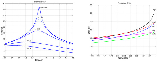
Figure 1.
(Left panel): Signal-to-noise ratio (SNR) as a function of line slope for fixed values of the correlation coefficient . (Right panel): Signal-to-noise ratio (SNR) as a function of correlation coefficient , for fixed values of the line slope .
- As , , when . In this region, changes vary rapidly as small variations in give very large variations in (left panel).
- As , for the values of shown, is practically a constant (right panel).
These features do affect the “self-noise” present in “self-channels” and the “cross-noise” present in “cross-channels” discussed in Section 4 and Section 5.
Before studying, in depth, a particular linguistic channel (namely the “sentences channel”) in Section 4, let us recall the graphical representation of deep-language variables as vectors in the vector plane, by applying it to Matthew.
3. Vector Analysis of Translations Based on Deep-Language Variables
Independently of the different parallel channels (one for each variable), the correlation noise () in most cases is larger than the regression noise (), therefore indicating that every translation tries as much as possible to be not biased, i.e., to approach , but it cannot avoid to be decorrelated (), with correlation coefficients which approximately decrease in the regression lines related to characters, words, sentences, interpunctions and to , , and .
If different translations of a New Testament text into the same language can be mathematically quite different, this is always found for different languages [1], as we explicitly show now for Matthew by using a graphical tool developed in [2], namely the vector plane.
The vector plane is a useful graphical tool for synthetically comparing different literary texts. As it can be noticed in Figure 18 of [39], for most Tew Testament texts the vector plane allows to assess how much different texts are mathematically similar, by considering the four deep-language variables , , , not explictly controlled by authors when writing. It considers the following six vectors of components and given by the average values of the variables: ), ), ), ), ), ) and their resulting vector, of coordinates and , given by:
Table 1 reports the average values of , , , found in Matthew in the indicated languages. Figure 2 shows the vector plane reporting and of Equation (13), and Figure 3 shows the distance of a translation from the Greek Matthew (, for each language. Latin, as it was found in [1], is the translation closest to the original Greek. From these figures we can see that all translations are mathematically quite diverse from the original Greek text and show a large variability, as in [1]. Similar results can be found for other New Testament texts, here not considered for brevity.

Table 1.
Average values of (characters per word), (words per sentence), (words per interpunction), (interpunctions, or number of , per sentence) in Matthew, in the indicated languages.
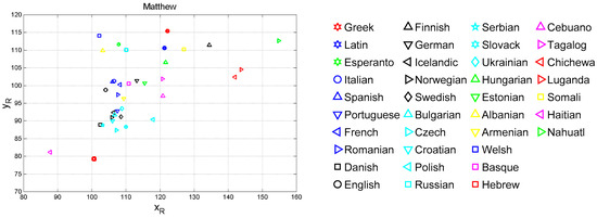
Figure 2.
(Left panel): Vector plane and of all languages concerning Matthew; for Greek ; . (Right panel): Graphical symbols referring to the indicated languages.
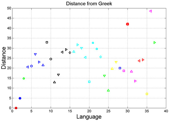
Figure 3.
Distance from Matthew according to the language indicated in abscissa. The order of languages is the same as in Table 1. Greek (language no.1) is at ; Latin (2) at ; English (10) at , etc.
It is interesting to notice that, in any language family (Table 1), varies in a range of approximately 7 dB. Some translations in some language families practically coincide, e.g., Italian, French and Spanish, or Icelandic, Norwegian and Swedish.
Because it is cumbersome to consider all New Testament texts studied in [1] to assess whether, within a language, the mathematical mutual relationships of the original Greek texts are saved or lost, in the following we use only Matthew as reference text in any language. From the large spread shown in Figure 1, we can imagine the even large spread likely found in studying all langauges, a topic, however, deeply studied in [1].
In conclusion, the results reported below, by assuming Matthew as reference text, are sufficient for giving a reliable answer to the issues mentioned in the Introduction.
In other words, for the purpose of being specific in deriving the full characteristics of the extended theory, it is sufficient to consider only Matthew and its translations, to show how a text is mathematically related, within the same language, to other texts, namely, in the following, the gospel according to Mark (Mk), Luke (Lk) and John (Jh), and to Acts (Ac) and Apocalypse (Revelation) (Ap).
Moreover, of the many linguistic channels linking two texts, for brevity we consider the channel that links their sentences, discussed in the next section.
4. The Sentences Channel and Its Theoretical Signal-to-Noise Ratio
“Translation” can also refer-as discussed in Section 2- to the case in which a text is compared to another text both written in the same language. We can investigate, for instance, how the number of sentences in text is “translated” into the number of sentences in text for the same number of words. This comparison can be done, of course, by considering average values and regression lines, but now the theory allows us to consider also the correlation coefficient-i.e., the noise defined in Equation (5)-and provides insight because it models linguistic channels according to parameters of communication theory, such as the signal-to-noise ratio (and possibly channel minimum capacity [1]). For our study of the several linguistic channels we consider, for illustration, only the sentences channel.
Let us consider the Greek texts of the New Testament, and let us compare Matthew, in turn, to Mark, Luke, John, Acts and Apocalypse.
Notice that in any translation, all texts have been worked as detailed in [1]. For each chapter, we have counted words, sentences and interpunctions (full-stops, question marks, exclamation marks, commas, colons, semicolons) after deleting all extraneous characters added to the original text by translators/commentators, such as titles, footnotes et cetera. At the end of this lengthy and laborious work, only the original text was left to be studied. Of course, it is not required to understand any of the translation languages–the theory does not consider meaning-because the process consists in just counting characters and sequences of characters. In the end, for example, in any language, Matthew is made of 28 chapters, therefore all regression lines, or any other data processing, are always based on 28 couples of data.
According to Section 2, to apply the theory to the sentences channel, we need to know the slope and the correlation coefficient of the regression line between the number of sentences per chapter (dependent variable) and the number of samples of another variable (independent variable) for each text. As independent variable, we consider the number of words per chapter, therefore the input parameters refer to the regression line between sentences () and words (). By eliminating words, the theory compares sentences for equal number of words, i.e., studies the sentences channel.
For example, Table 2 shows the regression parameters found in the original Greek texts. Notice that we have maintained 4 decimal digits because some values differ only from the third digit. For example, on the average, for 100 words we find sentences in Matthew, sentences in Luke (the text closest to Matthew when considering all deep-language variables, as reported in [39]) and only sentences in Apocalypse.
Table 2.
Line slope (sentences per word) and correlation coefficient of the regression line between words (independent variable) and sentences (dependent variable) in the indicated New Testament Greek texts. We have reported 4 decimal digits because some values differ only from the third digit.
Because we always consider Matthew as dependent text, the data of Table 2 can be used to compare the sentences channel of Matthew with itself (self-channel) and with the other texts (cross-channels). Mathematically, the input data (reference, independent data) to the theory are the slope and the correlation coefficient given, in turn, by Mark (e.g., and , Luke, John, Acts and Apocalypse, and the dependent data are always the values of Matthew, therefore and . Table 3 reports, for each cross-channel, the values of –calculated with Equation (4)-and –calculated with Equation (8)–and the total signal-to-noise ratio calculated with Equations (11) and (12), and the partial values and , calculated with Equations (6), (7), (9) and (10).
Table 3.
Values of –calculated with Equation (4)-and –calculated with Equation (8)–and the total signal-to-noise ratio calculated with Equations (11) and (12), and the partial values and , calculated with Equations (6) (7), (9) and (10) in the indicated cross-channels.
For example, according to Table 3, the number of sentences estimated in Matthew is given by the number of sentences in Luke multiplied by , with correlation coefficient . Therefore, the fraction (98.76%) of the variance of the sentences in Matthew is due to the regression line, while only (1.24 %) is due to decorrelation. The large difference between the partial signal-to-noise ratios and make the total value , practically determined by , because in Equation (11) .
For the values linked by the regression line (see ), Matthew is closer to Luke than to Mark (the other synoptic gospel) or to John, but when considering also the correlation coefficient, a different situation emerges (see as Matthew is closer to John than to Mark or Luke, although these differences are small and might be due to the statistical noise because of the small number of samples (28) in establishing the data of Table 2 (see Section 5).
Let us apply the theory to all languages. Figure 4, Figure 5 and Figure 6 show how changes with language when Matthew is compared to Mark, Luke, Acts and Apocalypse (cross channels; color key: blue = Mt vs. Mk; red = Mt vs. Lk; magenta = Mt vs. Jh; green = Mt vs. Ac; black = Mt vs. Ap).
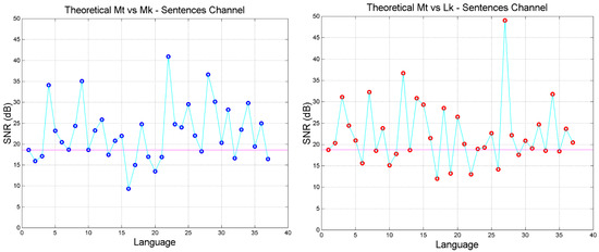
Figure 4.
Sentences cross-channel theoretical signal-to-noise-ratio in the indicated languages. Languages are ordered according to Table 1. (Left panel): Matthew versus Mark; (Right panel): Matthew versus Luke. The magenta line corresponds to Greek (language no.1). In these figures, and also in the following, the continuous lines serve for guiding eyes.
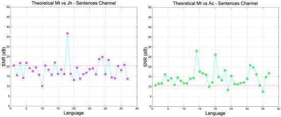
Figure 5.
Sentences cross-channel theoretical signal-to-noise-ratio in the indicated languages. Languages are ordered according to Table 1. (Left panel): Matthew versus John; (Right panel): Matthew versus Acts. The magenta line corresponds to Greek (language no.1).
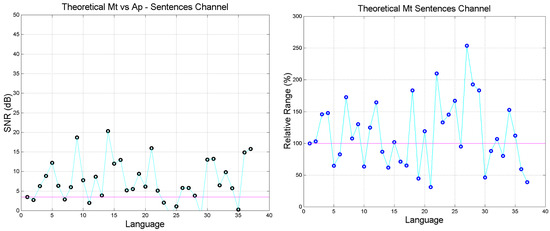
Figure 6.
(Left panel): Sentences cross-channel theoretical signal-to-noise-ratio in the indicated languages; Matthew versus Apocalypse. Languages are ordered according to Table 1. (Right panel): Sentences channel relative range (%) in the indicated languages. The magenta line corresponds to Greek (language no.1).
We can make the following general remarks:
- The signal-to-noise of both self- and cross-channels depends very much on language, with some translations giving significantly larger (more common) or smaller values than the Greek (language no.1).
- Only few translations are very similar to Greek, as their in the cross-channels falls on the magenta line, especially in Mt vs. Mk and Mt vs. Luke. For Mt vs. Mk they are: Romanian (language number 7), English (10), Armenian (27), Somali (35). For Luke: Spanish (8), Icelandic (13), Ukrainian (23), Estonian (24), Cebuano (31), Chichewa (33), Somali (35).
- The range of can be quite different from language to language, and can be biased, i.e., displaced mostly upwards (Mk, Lk, Ac, Ap) or mostly downwards (Jh), compared to Greek.
Figure 6 shows (right panel) also the relative range (%) found in a language, i.e., the range of () divided by the range in the Greek texts. The relative range can be largely compressed (below the magenta line) or expanded (above the magenta line), therefore biasing readers’ style appreciation of texts. Very few languages maintain the range of Greek texts, namely Latin (2), Swedish (15), Albanian (26), Tagalog (32). In other words, texts which in Greek are mathematically quite different, in another language can be very similar, or vice versa.
However, at this point some important observations must be highlighted. The slope and correlation coefficient of a regression line are stochastic variables, therefore characterized by average values (e.g., those reported in Table 2 for Greek, calculated by standard algorithms) and standard deviations. The extended theory would yield improved estimates, of course, if the standard deviation were a very small percentage of the average value. However, with a sample size of at most 28 (as in Matthew, and even fewer samples in the other New Testament texts), the standard deviations of and can give too large variations in predicted by the theory and reported in Table 3 and in Figure 4, Figure 5 and Figure 6.
Because the largest values of fall in the steepest region of Figure 1, a small statistical fluctuations in or in , or in both, are amplified in . Only when the input parameters are more diverse, as with Acts and Apocalypse (Table 2), the larger mathematical distinction is maintained ( dB and dB, respectively) because in this case falls in the flat region of Figure 1 and the total noise effectively tends to mask sensitivity to or to .
To avoid this inaccuracy-due to the small sample size from which the regression lines are calculated (see Appendix B), not to the theory of Section 2-, we adopt a kind of “renormalization” based on Monte Carlo simulations-whose results we consider as “experimental”-defined and discussed in the next section.
5. The Sentences Channel and Its Experimental Signal-to-Noise Ratio
If we compare Matthew with itself (self-channel), we consider the ideal channel, therefore , and , values of no practical use. Therefore, we suggest to use a Monte Carlo simulation for three purposes: (a) renormalize the self-channel to get a finite reference signal-to-noise ratio to which compare self-channels and cross-channels; (b) to mitigate the inaccuracy in the regression lines of the texts (cross-channels) to which Matthew is compared; (c) to assess the maximum theoretical signal-to-noise ratio conservatively reliable, i.e., not likely due to chance.
In this section we first set and run the simulation and secondly, we define and discuss the experimental self- and cross-channel signal-to-noise, whose characteristics may be useful to distinguish between two texts.
5.1. Monte Carlo Simulation and Experimental Signal-to-Noise Ratio
In this subsection we define the steps in the Monte Carlo simulation and calculate the signal-to-noise ratio. Let us:
- Generate 28 (the number of chapters in Matthew) independent numbers from a discrete uniform probability distribution in the range 1 to 28, with replacement–i.e., a number can be selected more than once.
- “Write” another possible “Matthew” with new 28 chapters corresponding to the numbers of the list randomly extracted; e.g., 23; 3; 16… hence take chapter 23, followed by chapter 3, chapter 16 etc. The text of a chapter can appear twice (with probability ), three times (with probability ), et cetera, and the new Matthew can contain a number of words greater or smaller than the original text, on the average (the differences are small and do not affect the results).
- Calculate the parameters and of the regression line between words (independent variable) and sentences (dependent variable) in the new Matthew.
- Consider the values of so obtained as “experimental” results , to be compared to the theoretical results of Section 4. Notice that it is not necessary to generate also new “Mark”, “Luke” et cetera, because we wish to compare the theoretical results of Section 4 to the results found in this section, therefore the input and must be the same.
- Repeat steps 1 to 5 many times (we did it 5000 times).
Besides the usefulness, as we show below, of the simulation as a “renormalization” tool of Matthew, the new texts obtained in step (2) might have been written by the author of the original text because they maintain, on the average, the statistical relationships between the linguistic variables of the original text. In other words, the simulation should take care of the inaccuracy in estimating slope and correlation coefficient due to a very limited sample size by considering a larger sample size of texts which might have been written by the same author.
For example, Figure 7 (left panel) shows, for Greek, the scatter plot between and the slope of the regression line of step 3. The samples are spread according to the value of the correlation coefficient found in step 3, and follow the theoretical curves shown in Figure 1.
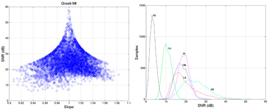
Figure 7.
(Left panel): Scatter plot between (SNR) and the slope of the regression line (step 3 of the Monte Carlo simulation) obtained in Greek. (Right panel): Probability distributions (histograms) of in the experimental self-channel (Matthew) and in the experimental cross-channels. Mt vs. Mk (blue), Mt vs. Lk (red), Mt vs. Jh (magenta), Mt vs. Ac (green) and Mt vs. Ap (black).
Table 4 reports the average values and standard deviations of of the self-channel-any new Matthew is compared to Matthew with regression line parameters and -, and for the cross-channels-any new Matthew is compared to Mark, Luke etc.-whose regression line parameters (input data) are listed in Table 2.
Table 4.
Average value and standard deviation (dB) of the experimental (simulation) in Mt self- and cross-channels.
Notice that the average value of Mt vs. Lk (19.52 dB) is now closer to Matthew (Mt vs. Mt) and that the standard deviation of Mt vs. Mt (6.84 dB) and Mt vs. Lk (6.20) are very alike and significantly larger than those of the other cross-channels. In other words, these findings indicate a larger similarity of Matthew with Luke than with other texts, in agreement with what reported in [21], and also that the sentences channel is reliable.
Figure 7 shows also (right panel) the probability distributions (histograms) of in the experimental self-channel (Matthew) and cross-channels. Similar results (not shown for brevity) are also found when the other New Testament texts (Mark, Luke etc.) are taken as output texts to be used in the simulation, whose Greek self-channels values are reported in Table 5.
Table 5.
Average value and standard deviation of (dB) in the indicated Greek self-channels.
Returning to Table 4, we can notice that the standard deviation decrease in the cross-channels in the order Lk, Mk, Jh, Ac, Ap. The concentration of the histograms in a narrow range in Figure 7 (small standard deviation) is mainly due to the large change in , e.g., in Mt vs. Ap (Table 3). Now the data spreading along the regression line appear to be “compressed” when texts with very different slope are used as output, such as with Matthew. We can see, on the contrary, that the standard deviation of the Greek self-channels of all texts (Table 5) are about the same. In other words, the fact that the probability distribution of decreases both in its average value and standard deviation when passing from self-channels to cross-channels is general.
In self-channels (Table 5), the average value depends on the text, but the standard deviation is practically very alike for all texts, in the range dB. Notice that the self-channel standard deviation of Luke, dB, is very close to the value, dB, found in the cross-channel Mt vs. Lk reported in Table 4. This further show that Luke is closer to Mt, than to the other texts.
Finally Figure 8 shows obtained in Matthew self-channel and in its cross-channels, for all languages. Languages are ordered according to Table 1. Figure 9 shows the difference between in Matthew self-channel and that in the cross-channels, for all languages. We can notice how, in most languages, the difference is very different from the difference found in Greek (language no.1). Moreover, in some languages the difference between in Mt vs. Mt and in Mt vs. Lk is practically 0 dB so that, in these languages–at least for the sentences channel-Matthew coincide, mathematically, with Luke therefore amplifying what is found in Greek, namely that Matthew is more similar to Luke than to other texts. These results mostly agree with those found in the theoretical cross-channels, as we show in the next sub-section.
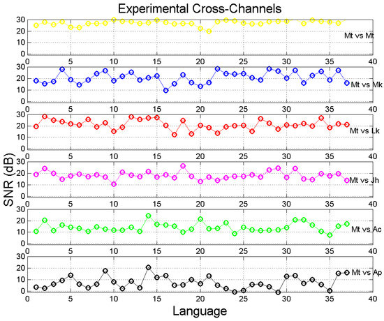
Figure 8.
Experimental signal-to-noise-ratio in Matthew self-channel and in its cross-channels in the indicated languages. Languages are ordered according to Table 1. Color key: yellow = Mt vs. Mt; blue = Mt vs. Mk; red = Mt vs. Lk; magenta = Mt vs. Jh; green = Mt vs. Ac; black = Mt vs. Ap.
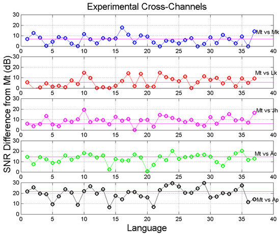
Figure 9.
Difference between in the self-channel (Mt vs. Mt) and that in the cross-channels, for all languages, according to Figure 8. Languages are ordered according to Table 1. The magenta lines correspond to Greek (1). Color key: blue = Mt vs. Mk; red = Mt vs. Lk; magenta = Mt vs. Jh; green = Mt vs. Ac; black = Mt vs. Ap.
5.2. Experimental versus Theoretical Signal-to-Noise Ratio
Very interesting is the comparison between the theoretical (Section 4) and the experimental signal-to-noise . For all languages and cross-channels, Figure 10 shows the scatter plot between and (left panel) and the difference (right panel), which estimates the ratio (expressed in dB) between the total noise power in the experimental channel and that in the theoretical channel. The horizontal magenta line reports, for reference, the average value of Matthew self-channel (see Table 5).
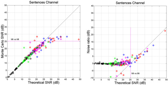
Figure 10.
(Left panel): Scatter plot between the theoretical total signal-to-noise ratio and for the indicated cross-channels. (Right panel): Difference , i.e., ratio (expressed in dB) between the noise power in the experimental channel and that in the theoretical channel. Color key: blue = Mt vs. Mk; red = Mt vs. Lk; magenta = Mt vs. Jh; green = Mt vs. Ac; black = Mt vs. Ap. The magenta line corresponds to Greek self-channel.
We can notice the following characteristics:
- For several languages, cross-channel maxima are found in Mt vs. Mk and in Mt vs. Lk, in the approximate (ordinate) range dB.
- Very clearly, there is a horizontal asymptote, starting at about this range contains most values of of self-channels (see Table 5).
- Before saturation, (approximately a 45°-line). Therefore, for dB, theory and simulation agree, indicating that the values of slope and correlation coefficient which determine are sufficiently accurate to be used conservatively as input to the theory, without performing a Monte Carlo simulation.
- The difference tends to be constant before saturation; afterwards it increases linearly.
Let us now compare the theoretical signal-to-noise ratios and to . Figure 11 () and Figure 12 ( show the scatter plots. We can observe characteristics similar to those shown in Figure 9, but with a significant larger spread. In Figure 10 saturation occurs at higher value of the signal-to-noise ratio ( dB) because, as we have shown in Table 3, is usually larger than . In Figure 12 the saturation occurs practically at the same value of Figure 10 because in most cases .
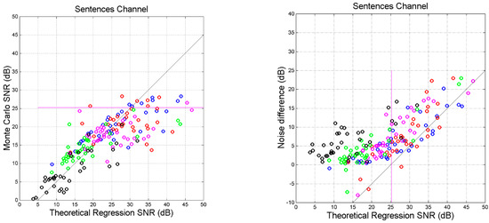
Figure 11.
(Left panel): Scatter plot between the theoretical partial signal-to-noise ratio and the experimental in the indicated cross-links. (Right panel): Difference , i.e., the ratio (expressed in dB) between the noise power in the experimental channel and that in the theoretical channel. Color key: blue = Mt vs. Mk; red = Mt vs. Lk; magenta = Mt vs. Jh; green = Mt vs. Ac; black = Mt vs. Ap. The magenta line corresponds to Greek self-channel.
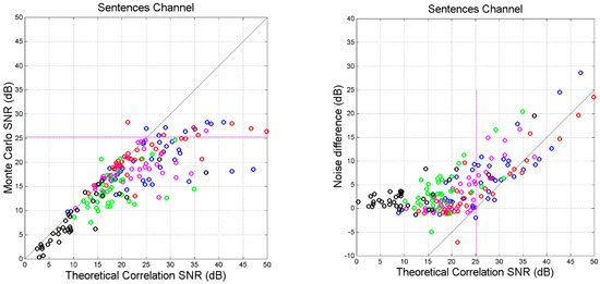
Figure 12.
(Left panel): Scatter plot between the theoretical partial signal-to-noise ratio and the experimental in the indicated cross-links. (Right panel): Difference , i.e., the ratio (expressed in dB) between the noise power in the experimental channel and that in the theoretical channel. Color key: blue = Mt vs. Mk; red = Mt vs. Lk; magenta = Mt vs. Jh; green = Mt vs. Ac; black = Mt vs. Ap. The magenta line corresponds to Greek self-channel.
In the next section we discuss how changes in self- and cross-channels when the output text is reduced. The study may be useful to further indicate whether two texts are mathematically indistinguishable.
6. Self-and Cross Channels Signal-to-Noise Ratios in Reduced Texts
Let us study how the signal-to-noise ratio changes in self- and cross-channels when the output text is reduced. This analysis can be useful for indicating whether two texts are mathematically indistinguishable.
For this analysis, we perform a Monte Carlo simulation like that described in Section 5, but now the number of chapters is varied from maximum (28 for Matthew) to a minimum of at least 3. Then, for each text reduction, we calculate the experimental values of , and as outlined in Section 5.
Figure 13 (left panel) shows the average values of , and as a function of the fraction of text considered, the latter given by the average total number of words found in the simulation with reduced text divided by the total average number of words found in the simulation with full text (28 chapters). The normalization to 100% takes care of the small differences in totals mentioned in Section 5.
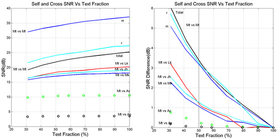
Figure 13.
(Left panel): Average values of (total), (m) and (r), versus fraction of text considered in Matthew self-channel and total in the cross-channels indicated. (Right panel): Difference between the average signal-to-noise ratio obtained with full text (100%) and that obtained with reduced text in the same channels.
We notice that in the self-channel the total signal-to-noise ratio is practically determined more by than by , as already observed for full text (Table 3). The cross-channels follow a similar trend but with a very important difference, highlighted in Figure 13 (right panel), which shows the difference between the 100% signal-to-noise ratio and that at the indicated fraction. The most striking finding is that in the self-channel at , and are all reduced by 3 dB. In other words, in a large range of , , and are proportional to .
On the contrary, the reduction is much lower in the cross-channels, whose results are also shown in Figure 13 (right panel). Mathematically this is due to being in the steepest range of Figure 1 in the self-channel-where signal-to-noise ratio drops rapidly -, and in the flat range in the cross-channels. This is confirmed by the results shown in Figure 14, which clearly shows that, the slope is practically constant, regardless of , while the correlation coefficient varies significantly.
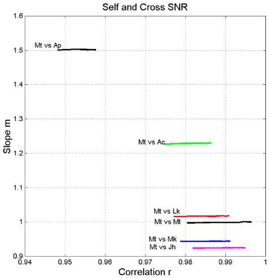
Figure 14.
Scatter plot between correlation coefficient and line slope for Matthew self-channel (Mt vs. Mt) and Matthew cross-channels Mt vs. Mk (blue), Mt vs. Lk (red), Mt vs. Jh (magenta), Mt vs. Ac (green), Mt vs. Ap (black).
This characteristic can be considered as another check to assess whether a text can be confused with another text, be therefore indistinguishable, a characteristic more stringent than mere similarity of , such that between Matthew and Luke. In other words, if in a self-channel and in its cross-channels , and are proportional to , then we can be reasonably confident that the two texts are more than similar, than one can be confused with the other, not excluding the further hypothesis that the author is the same.
The same characteristics can be found in any text. For example, Figure 15 shows the results found in the self-channels concerning the Greek Jewish War (JW) by Flavius Josephus, the English David Copperfield (DC) by Charles Dickens, and the Italian I Promessi Sposi (PS) by Alessandro Manzoni. For each text, regardless of epoch and language, the total signal-to-noise ratio is reduced according to .
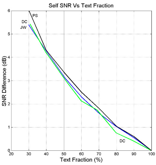
Figure 15.
Difference between the average signal-to-noise ratio obtained with full text (100%) and that obtained with reduced text in the sentences self-channel in Jewish War (JW, blue line), David Copperfield (DC, green line), and I Promessi Sposi (PS, black line).
7. Channel Probability of Error and Likeness Index
In this section we explore a way of comparing the signal-to-noise ratios of self- and cross-channels objectively and automatically, and possibly also getting more insight on texts mathematical likeness.
In the sentences channel explicitly studied in the present paper-but our development can be applied to any other linguistic channel-, can we “measure” how close, in the Monte Carlo simulations, is Matthew to itself (self-channel), or to other texts (cross-channels) with an index based on probability? In other words, how much can we be confident that a text can be mistaken, mathematically, with another text, e.g., Matthew with Luke or John, et cetera, by studying self- and cross-channels? Because in the Monte Carlo simulations we get probability densities as those shown in Figure 7 (right panel) for Greek, we must deal with continuous functions. In other words, can Mt self- channel, described statistically by its probability density shown in Figure 7, be confused with one of the cross- channels, also described by a probability density in Figure 7, therefore implying, for example, that Matthew and Luke are very similar, while Matthew and Acts are not? The probability problem is binary because a decision must be taken between two alternatives.
The problem is classical in binary digital communication channels affected by noise, as recalled in Appendix C. In this field, “error” means that bit 1 is mistaken for bit 0 or vice versa, therefore the channel performance worsens as the error frequency (i.e., the probability of error) increases.
Now, in the sentence self- and cross channels-to be specific -, “error” means that a text can be more or less mistaken, or confused, with another text, consequently two texts are more similar as the probability of error increases.
According to Equation (A8), the average minimum probability of error in a binary channel with equiprobable “events”–as we assume, of course, for self- and cross-channels-is given by:
In Equation (14) and are the signal-to-noise ratios in the indicated channels.
The decision threshold , as shown in Appendix C, is given by the intersection of the known probability density functions (cross-channel) and (self-channle), i.e., the experimental probability densities shown in Figure 7. The integrals limits are fixed as shown in Equation (14) because .
Let us study the range of If there is no intersection between the two densities; their average values are centered at and , respectively, or the two densities have collapsed to Dirac delta functions. If the two densities are identical, e.g., a self-channel is comparerd with itself. In conclusion, . Therefore, when cross- and self- channels can be considered totally uncorrelated; when , self and cross-channels coincide, the two texts are mathematically identical.
Instead of reporting results on , we define and show results of the following normalized “likeness index” :
In Equation (15), ; means totally uncorrelated texts, means totally correlated texts.
Let us apply Equation (15) to the probability density of (“bit 1”) and (“bit 0”). Now, according to Figure 7 (right panel), and can be well modelled in a large range with Gaussian probability density functions (not shown for brevity), with average value and standard deviations given by Table 4 in Greek Matthew self- and cross-channels.
In the left panel of Figure 16 we show in the indicated cross-channels (i.e., ) compared to Matthew self-channel (i.e., . It is evident that when the text of Matthew is referred to Luke (Mt vs. Lk, red line) is the closest to Matthew self-channel (Mt vs. Mt): in other words, Matthew can be confused with Luke (and vice versa) more than with Mark, John, Acts or Apocalypse.

Figure 16.
vs. text fraction considered in the Monte Carlo simulations in Greek. (Left panel): Matthew self-and cross-channels; color key in left panel: red refers to cross-channel Mt vs. Lk, blue to Mt vs. Mk, magenta to Mt vs. Jh, green to Mt vs. Ac, black to Mt vs. Ap; refers to Mt self-channel. (Right panel): Matthew and Luke self- and cross-channels; color key in right panel: red lines refer to cross-channel compared to Mt self-channel; green lines refer to cross-channels compared to Lk self-channel. refers to Mt self-channel (indicated by/Mt) or to Lk self-channel (indicated by/Lk).
The results shown in the right panel of Figure 16 highlight the asymmetry of linguistic channels [1]. Here we show cross- and self-channels of both Matthew and Luke referred to their self-channels. For example, of the cross-channel in which Matthew is “read” as Luke and compared to Luke (Mt vs. Lk/Lk, solid green line) is smaller than of the cross-channel in which Luke is “read” as Matthew (Lk vs. Mt/Mt) and compared to Matthew.
From Figure 16, we can draw the following conclusions on a possible use of the likeness index:
- (a)
- In the self-channel Mt vs. Mt, , for any text fraction (, therefore 30% of Matthew compared with its full text retains a large likeness.
- (b)
- In the cross-channel Mt vs. Lk, for full-texts (100%), therefore indicating a large likeness when the full Mt is compared to the full Lk.
- (c)
- In the reverse channel Lk vs. Mt/Mt, for (right panel), therefore indicating a larger likeness when Luke is compared to Matthew.
- (d)
- In the cross-channel Lk vs. Mt/Lk (right panel) the likeness index is markedly larger than in the cross-channel Mt vs. Lk/Mt. This finding may support the conjencture, shared by many scholars (see [39]), that Matthew was written before Luke, and that Luke might have known Matthew when he wrote his text.
- (e)
- In the cross-channels Mt vs. Mk and Mt vs. Jh .
- (f)
- In the cross-channels Mt vs. Ac and in Mt vs. Ap .
In conclusion, the likeness index seems reliable because it confirms known relationships among the Greek New Testament texts (e.g., [39]). In particular it confirms that Matthew and Luke are the most similar texts.
Similar results are found in English, shown in Figure 17 where refers to Mt self-channel. Compared to Greek (Figure 16, left channel), distortions are clearly evident because is quite smaller, and with different rankings, than what found in Greek.
Figure 17.
vs. text fraction in Matthew self- and cross-channels, in English. In Mt vs. Lk cross-channel (solid red line) Matthew is compared to Luke; in the reverse channel Lk vs. Mt (solid red line with circles), Luke is compared to Matthew. refers to Mt self-channel.
Finally notice the universal result that in self-channels is practically given by the same function, for and for , features which evidently characterize self-channels, as also shown in Section 8.
In conclusion can be considered another usefull index for automatically comparing texts in a multidimensional space of indices.
8. Texts across Time
In this section we first compare the following translations of Matthew: (a) modern English-version studied in the present paper-versus the XVII century English of King James’ Bible; (b) modern German-version studied in the present paper- versus the XVI century German of Luther’s Bible. All texts have been downloaded from the web sites reported in [1]. Secondly, we compare the two versions of the Italian novelist Alessandro Manzoni’s masterpiece, namely Fermo e Lucia (Fermo and Lucy) and I Promessi Sposi (The Betrothed).
Figure 18 shows versus text fraction for English (left panel) and for German (right panel). Besides the trend of self-channels already observed in Figure 16 and Figure 17 ( for any and for ), the two versions of Matthew seem to refer to different texts because the cross-channels have very small , practically the same value found in the cross-channels Mt vs. Ac or Mt vs. Ap in Greek (Figure 16, left panel). Similar results are found also for German, with in both cross-channels.
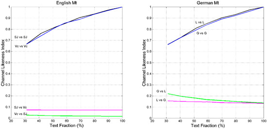
Figure 18.
vs. text fraction in Matthew self- and cross-channels. Left panel: Modern English (Vc)-version studied in the present paper-versus the XVII century English of King James’ Bible (SJ). In the cross-channel Vc vs. SJ (green line) refers to King James.; in the cross-channel SJ vs. Vc (magenta line) refers to modern English. Right panel: Modern German (G)-version studied in the present paper- versus the XVI century German of Luther’s Bible (L). In the cross-channel G vs. L (green line) refers to Luther; in the cross-channel L vs. G (magenta line) refers to modern German. All texts have been downloaded from the web sites reported in [1].
From Figure 18, we can conclude that the modern translations of Matthew in English and in German are signficantly different of the classical versions due to King James (English) and to Luther (German).
Alessandro Manzoni (Milan 1785, Milan 1873), one of the most studied Italian novelist and poet in Italian High Schools and Universities, in 1827 published Fermo e Lucia, a text that scholars of Italian Literature-and Manzoni himself- consider the “first” version of his masterpiece I Promessi Sposi, which was published in 1842. According to scholars, the two versions differ very much, both for structure and characters [40,41,42,43], therefore it is interesting to study how much the author transformed (mathematically) Fermo e Lucia into I Promessi Sposi, according to our theory specifically applied to the sentences channel.
Figure 19 shows versus text fraction for the indicated self- and cross-channels. The novel published in 1842 (PS) has practically little connection with that (FL) published in 1827, as scholars of Italian Literature have noticed.
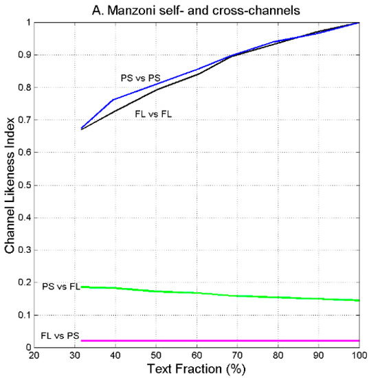
Figure 19.
vs. text fraction in Alessandro Manzoni’s novels. FL = Fermo e Lucia; PS = I Promessi Sposi. In the cross-channel Ps vs. FL (green line) refers to Fermo e Lucia. In the cross-channel FL vs. PS (magenta line) refers to I Promessi Sposi.
9. Concluding Remarks
We have extended the general theory of translation [1] to texts written in the same language. To be specific, we have applied the extended theory to New Testament translations already studied in [1], and have assessed how much the mutual linguistic mathematical relationships present in the original Greek texts have been saved or lost in 36 languages. In general, we have found that in many languages/translations the original relationships have been lost and consequently texts have been mathematically distorted.
After defining the mathematical problem in general terms, we have assessed the sensitivity of the signal-to-noise ratio of a linguistic channel to input parameters. The theory is based on the properties of linear regression lines, therefore on slope and correlation coefficient . The slope is the source of the “regression noise”–because ; the correlation coefficient is the source of the “correlation noise”–because , as discussed in [1] for translation channels, but now the theory refers also to texts written in the same language.
Because it is cumbersome to consider all New Testament texts to assess whether, within a language, the mathematical mutual relationships of the original Greek texts are saved or lost, we have studied only the gospel according to Matthew as reference text in any language. However, the results reported are sufficient for giving a reliable answer to the question.
For the purpose of being specific in deriving the full characteristics of the extended theory, we have shown how Matthew is mathematically related, within the same language, to the gospels according to Mark (Mk), Luke (Lk) and John (Jh), and to Acts (Ac) and Apocalypse (Revelation) (Ap). The channels so defined are termed “cross-channels”. The channel in which Matthew is compared with itself is the “self-channel”.
Of the many linguistic channels linking two texts [1], we have considered only the channel that links their sentences, referred to as the “sentences channel”. We have investigated how the number of sentences in text is “translated” into the number of sentences in text for the same number of words. This comparison can be done, of course, by considering average values and regression lines, but the theory has allowed us to consider also the correlation coefficient and has provided insight because it models linguistic channels according to parameters of communication theory, such as the signal-to-noise ratio.
To avoid the inaccuracy, due to the small sample size from which the regression lines are calculated, we have adopted a kind of “renormalization” based on Monte Carlo simulations, whose results we consider as “experimental”. We have compared theoretical and experimental signal-to-noise ratios and have found that for several languages cross-channel maxima are found in the approximate (ordinate) range dB. Beyond these values there is saturation, i.e., a horizontal asymptote. Before saturation, (approximately a 45°-line). In other words, for dB, theory and simulation agree, indicating that the values of slope and correlation coefficient which determine are sufficiently accurate to be used conservatively as input to the theory, without performing a Monte Carlo simulation.
We have also studied how the signal-to-noise ratio changes when the output text is reduced, according to the fraction . This analysis can be useful for indicating whether two texts are mathematically indistinguishable. We have found that the signal-to-noise ratio in the self-channel is proportional to . In the cross-channels the reduction is much lower. Operationally, this can be another check to assess whether a text can be confused with another text.
We have found the same characteristics in self-channels concerning the Greek Jewish War (JW) by Flavius Josephus, the English David Copperfield (DC) by Charles Dickens, and the Italian I Promessi Sposi (PS) by Alessandro Manzoni. For each text, regardless of epoch and language, the total signal-to-noise ratio is reduced according to .
We have also we explored a way of comparing the signal-to-noise ratios of self- and cross-channels objectively and automatically-by applying concepts of binary communication channels affected by noise-, and possibly also a way of getting more insight on texts mathematical likeness. To this end, we have defined a “likeness index” , and have shown how it can reveal similarities or differences of different texts.
Finally notice that, because the theory deals with linear regression lines, it can be applied any time a scientific/technical problem involves two or more linear regression lines, therefore it is not limited to linguistic variables but it is universal.
Funding
This research received no external funding.
Institutional Review Board Statement
Not applicable.
Informed Consent Statement
Not applicable.
Data Availability Statement
The source of data used in this study is provided in the manuscript.
Conflicts of Interest
The authors declare no conflict of interest.
Appendix A. List of Mathematical Symbols
| Symbol | Meaning |
| number of characters per word | |
| fraction of text | |
| likeness index | |
| number of words per interpunction (word interval) | |
| slope of linear regression line | |
| number of interpunctions per sentence | |
| noise source | |
| number of sentences per chapter | |
| number of words per chapter | |
| correlation coefficient | |
| linguistic vector | |
| total noise-to-signal power ratio | |
| regression noise-to-signal power ratio | |
| correlation noise-to-signal power ratio | |
| number of words per sentence | |
| total number of sentences | |
| coordinate in the vector plane | |
| coordinate in the vector plane | |
| input language | |
| output language | |
| total number of words | |
| signal-to-noise power ratio in self- and cross-channels | |
| signal-to-noise power ratio in decibels | |
| experimental signal-to-noise power ratio (Monte Carlo simulation) | |
| regression signal-to-noise power ratio (due to ) | |
| correlation signal-to-noise power ratio (due to ) | |
| theoretical signal-to-noise power ratio |
Appendix B. Variability of Linear Regression Line Parameters
Let be a correlation coefficient of a regression line of a large sample size . According to statistical theory (see [44] p. 296), the transformed variable:
is approximately Gaussian, with average value given by Equation (A1) and variance given by:
Let us consider Matthew, hence and (Table 2). A sample size of 28 is not large. However, for the purpose of estimating some bounds, let us apply Equations (A1) and (A2). The parameters of the Gaussian distribution are therefore and . At , we find and From Equation (A1), we get:
From Equation (A3), we calculate at , 0.9601 and , a very large range.
A similar analysis, although more complicated, can also be done for the slope , which for large is also Gaussian.
Moreover, since the correlation noise does depend also on , see Equation (9), we should estimate a reliable bivariate probability distribution of and , a difficult task.
In conclusion, because of all these mathematical difficulties it is straighter and more reliable to turn to the Monte Carlo simulation defined in Section 5.
Appendix C. Minimum Probability of Error in Binary Decisions
The following analysis is typical of binary digital communication channels affected by noise (usually Gaussian) ([45], Section 4.3), in which the receiver must decide, by sampling the amplitude of the received signal+noise, whether the bit 0 or the bit 1 has been transmitted, usually with amplitude of the pulse carrying bit 1 larger (e.g., positive) than that carrying bit 0 (e.g., negative).
Let and be the known (conditional) probability densities of the amplitude received when bit 0 or bit 1 have been transmitted, with a-priori probability and respectively. The average (or total) probability of error-i.e., the probability of mistaking bit 0 for bit 1 or vice versa-is given by:
In Equation (A4), is the amplitude threshold used by the receiver to make a (“hard”) decision. If the sample is larger than , the decision is bit 1; otherwise is bit 0.
The unknown threshold is chosen by minimizing . By deriving Equation (A4) with respect to and setting it equal to zero, we get:
Therefore, the threshold value which minimizes Equation (A5) is given by the implicit equation in the variable :
If the two bits are equiprobale-as is usually assumed in digital communications, i.e., -then Equation (A6) gives:
In other words, is determined by the intersection of the two known probability density functions, therefore:
References
- Matricciani, E. A Statistical Theory of Language Translation Based on Communication Theory. Open J. Stat. 2020, 10, 936–997. [Google Scholar] [CrossRef]
- Matricciani, E. Deep Language Statistics of Italian throughout Seven Centuries of Literature and Empirical Connections with Miller’s 7 ∓ 2 Law and Short-Term Memory. Open J. Stat. 2019, 9, 373–406. [Google Scholar] [CrossRef] [Green Version]
- Elmakias, I.; Vilenchik, D. An Oblivious Approach to Machine Translation Quality Estimation. Mathematics 2021, 9, 2090. [Google Scholar] [CrossRef]
- Proshina, Z. Theory of Translation, 3rd ed.; Far Eastern University Press: Manila, Philippines, 2008. [Google Scholar]
- Trosberg, A. Discourse analysis as part of translator training. Curr. Issues Lang. Soc. 2000, 7, 185–228. [Google Scholar] [CrossRef]
- Warren, R. (Ed.) The Art of Translation: Voices from the Field; Northeastern University Press: Boston, MA, USA, 1989. [Google Scholar]
- Williams, I. A corpus-Based study of the verb observar in English-Spanish translations of biomedical research articles. Target. Int. J. Transl. Stud. 2007, 19, 85–103. [Google Scholar] [CrossRef]
- Wilss, W. Knowledge and Skills in Translator Behaviour; John Benjamins: Amsterdam, The Netherlands; Philadelphia, PA, USA, 1996. [Google Scholar]
- Gamallo, P.; Pichel, J.R.; Alegria, I. Measuring Language Distance of Isolated European Languages. Information 2020, 11, 181. [Google Scholar] [CrossRef] [Green Version]
- Barbançon, F.; Evans, S.; Nakhleh, L.; Ringe, D.; Warnow, T. An experimental study comparing linguistic phylogenetic reconstruction methods. Diachronica 2013, 30, 143–170. [Google Scholar] [CrossRef] [Green Version]
- Petroni, F.; Serva, M. Measures of lexical distance between languages. Phys. A Stat. Mech. Appl. 2010, 389, 2280–2283. [Google Scholar] [CrossRef] [Green Version]
- Gao, Y.; Liang, W.; Shi, Y.; Huang, Q. Comparison of directed and weighted co-occurrence networks of six languages. Phys. A Stat. Mech. Appl. 2014, 393, 579–589. [Google Scholar] [CrossRef]
- Liu, H.; Cong, J. Language clustering with word co-occurrence networks based on parallel texts. Chin. Sci. Bull. 2013, 58, 1139–1144. [Google Scholar] [CrossRef] [Green Version]
- Gamallo, P.; Pichel, J.R.; Alegria, I. From Language Identification to Language Distance. Phys. A 2017, 484, 162–172. [Google Scholar] [CrossRef]
- Pichel, J.R.; Gamallo, P.; Alegria, I. Measuring diachronic language distance using perplexity: Application to English, Portuguese, and Spanish. Nat. Lang. Eng. 2019, 26, 434–454. [Google Scholar] [CrossRef]
- Eder, M. Visualization in stylometry: Cluster analysis using networks. Digit. Scholarsh. Humanit. 2015, 32, 50–64. [Google Scholar] [CrossRef]
- Brown, P.F.; Cocke, J.; Della Pietra, A.; Della Pietra, V.J.; Jelinek, F.; Lafferty, J.D.; Mercer, R.L.; Roossin, P.S. A Statistical Approach to Machine Translation. Comput. Linguist. 1990, 16, 79–85. [Google Scholar]
- Koehn, F.; Och, F.J.; Marcu, D. Statistical Phrase-Based Translation. In Proceedings of the HLT-NAACL 2003, Main Papers, Edmonton, AB, Canada, 27 May 2003; pp. 48–54. [Google Scholar]
- Michael Carl, M.; Schaeffer, M. Sketch of a Noisy Channel Model for the translation process. In Silvia Hansen-Schirra, Empirical Modelling of Translation and Interpreting; Czulo, O., Hofmann, S., Eds.; Language Science Press: Berlin, Germany, 2017; pp. 71–116. [Google Scholar] [CrossRef]
- Shannon, C.E. A Mathematical Theory of Communication. Bell Syst. Techn. J. 1948, 27, 379–423. [Google Scholar] [CrossRef] [Green Version]
- Lavie, A.; Agarwal, A. Meteor: An Automatic Metric for MT Evaluation with High Levels of Correlation with Human Judgments. In Proceedings of the Second Workshop on Statistical Machine Translation, Prague, Czech Republic, 23 June 2007; pp. 228–231. [Google Scholar]
- Banchs, R.; Li, H. AM-FM: A Semantic Framework for Translation Quality Assessment. In Proceedings of the 49th Annual Meeting of the Association for Computational Linguistics: Human Language Technologies, Portland, OR, USA, 19–24 June 2011; Volume 2, pp. 153–158. [Google Scholar]
- Forcada, M.; Ginestí-Rosell, M.; Nordfalk, J.; O’Regan, J.; Ortiz-Rojas, S.; Pérez-Ortiz, J.; Sánchez-Martínez, F.; Ramírez-Sánchez, G.; Tyers, F. Apertium: A free/open-source platform for rule-based machine translation. Mach. Transl. 2011, 25, 127–144. [Google Scholar] [CrossRef]
- Buck, C. Black Box Features for the WMT 2012 Quality Estimation Shared Task. In Proceedings of the 7th Workshop on Statistical Machine Translation, Montreal, QC, Canada, 7–8 June 2012; pp. 91–95. [Google Scholar]
- Assaf, D.; Newman, Y.; Choen, Y.; Argamon, S.; Howard, N.; Last, M.; Frieder, O.; Koppel, M. Why “Dark Thoughts” aren’t really Dark: A Novel Algorithm for Metaphor Identification. In Proceedings of the 2013 IEEE Symposium on Computational Intelligence, Cognitive Algorithms, Mind, and Brain, Singapore, 16–19 April 2013; pp. 60–65. [Google Scholar]
- Graham, Y. Improving Evaluation of Machine Translation Quality Estimation. In Proceedings of the 53rd Annual Meeting of the Association for Computational Linguistics and the 7th International Joint Conference on Natural Language Processing, Beijing, China, 26–31 July 2015; pp. 1804–1813. [Google Scholar]
- Espla-Gomis, M.; Sanchez-Martınez, F.; Forcada, M.L. UAlacant word-level machine translation quality estimation system at WMT 2015. In Proceedings of the Tenth Workshop on Statistical Machine Translation, Lisboa, Portugal, 17–18 September 2015; pp. 309–315. [Google Scholar]
- Costa-jussà, M.R.; Fonollosa, J.A. Latest trends in hybrid machine translation and its applications. Comput. Speech Lang. 2015, 32, 3–10. [Google Scholar] [CrossRef] [Green Version]
- Kreutzer, J.; Schamoni, S.; Riezler, S. QUality Estimation from ScraTCH (QUETCH): Deep Learning for Word-level Translation Quality Estimation. In Proceedings of the Tenth Workshop on Statistical Machine Translation, Lisboa, Portugal, 17–18 September 2015; pp. 316–322. [Google Scholar]
- Specia, L.; Paetzold, G.; Scarton, C. Multi-level Translation Quality Prediction with QuEst++. In Proceedings of the ACL-IJCNLP 2015 System Demonstrations, Beijing, China, 26–31 July 2015; pp. 115–120. [Google Scholar]
- Banchs, R.E.; D’Haro, L.F.; Li, H. Adequacy-Fluency Metrics: Evaluating MT in the Continuous Space Model Framework. IEEE/ACM Trans. Audio Speech Lang. Process. 2015, 23, 472–482. [Google Scholar] [CrossRef]
- Martins, A.F.T.; Junczys-Dowmunt, M.; Kepler, F.N.; Astudillo, R.; Hokamp, C.; Grundkiewicz, R. Pushing the Limits of Quality Estimation. Trans. Assoc. Comput. Linguist. 2017, 5, 205–218. [Google Scholar] [CrossRef] [Green Version]
- Kim, H.; Jung, H.Y.; Kwon, H.; Lee, J.H.; Na, S.H. Predictor-Estimator: Neural Quality Estimation Based on Target Word Prediction for Machine Translation. ACM Trans. Asian Low-Resour. Lang. Inf. Process. 2017, 17, 1–22. [Google Scholar] [CrossRef]
- Kepler, F.; Trénous, J.; Treviso, M.; Vera, M.; Martins, A.F.T. OpenKiwi: An Open Source Framework for Quality Estimation. In Proceedings of the 57th Annual Meeting of the Association for Computational Linguistics: System Demonstrations, Florence, Italy, 28 July–2 August 2019; pp. 117–122. [Google Scholar]
- D’Haro, L.; Banchs, R.; Hori, C.; Li, H. Automatic Evaluation of End-to-End Dialog Systems with Adequacy-Fluency Metrics. Comput. Speech Lang. 2018, 55, 200–215. [Google Scholar] [CrossRef]
- Yankovskaya, E.; Tättar, A.; Fishel, M. Quality Estimation with Force-Decoded Attention and Cross-lingual Embeddings. In Proceedings of the Third Conference on Machine Translation: Shared Task Papers, Belgium, Brussels, 31 October–1 November 2018; pp. 816–821. [Google Scholar]
- Yankovskaya, E.; Tättar, A.; Fishel, M. Quality Estimation and Translation Metrics via Pre-trained Word and Sentence Embeddings. In Proceedings of the Fourth Conference on Machine Translation, Florence, Italy, 1–2 August 2019; pp. 101–105. [Google Scholar]
- Lindgren, B.W. Statistical Theory, 2nd ed.; MacMillan Company: New York, NY, USA, 1968. [Google Scholar]
- Matricciani, E.; Caro, L.D. A Deep-Language Mathematical Analysis of Gospels, Acts and Revelation. Religions 2019, 10, 257. [Google Scholar] [CrossRef] [Green Version]
- Mazza, A. Studi Sulle Redazioni de I Promessi Sposi; Edizioni Paoline: Milan, Italy, 1968. [Google Scholar]
- Giovanni Nencioni, N. La Lingua di Manzoni. Avviamento Alle Prose Manzoniane; Il Mulino: Bologna, Italy, 1993. [Google Scholar]
- Guntert, G. Manzoni Romanziere: Dalla Scrittura Ideologica Alla Rappresentazione Poetica; Franco Cesati Editore: Firenze, Italy, 2000. [Google Scholar]
- Frare, P. Leggere I Promessi Sposi; Il Mulino: Bologna, Italy, 2016. [Google Scholar]
- Papoulis, A. Probability & Statistics; Prentice Hall: Hoboken, NJ, USA, 1990. [Google Scholar]
- Haykin, S. Communication Systems, 4th ed.; John Wiley & Sons: Hoboken, NJ, USA, 2001. [Google Scholar]
Publisher’s Note: MDPI stays neutral with regard to jurisdictional claims in published maps and institutional affiliations. |
© 2022 by the author. Licensee MDPI, Basel, Switzerland. This article is an open access article distributed under the terms and conditions of the Creative Commons Attribution (CC BY) license (https://creativecommons.org/licenses/by/4.0/).