An Analytical and Numerical Detour for the Riemann Hypothesis

Abstract

From the functional equation $F\left(s\right)=F\left(1-s\right)$ of Riemann’s zeta function, this article gives new insight into Hadamard’s product formula. The function $S_1\left(s\right)=d\left(\ln F\left(s\right)\right)/ds$ and its family of associated $S_m$ functions, expressed as a sum of rational fractions, are interpreted as meromorphic functions whose poles are the poles and zeros of the $F$ function. This family is a mathematical and numerical tool which makes it possible to estimate the value $F\left(s\right)$ of the function at a point $s=x+iy=\dot{x}+½+iy$ in the critical strip $𝒮$ from a point $𝓈=½+iy$ on the critical line $ℒ$. Generating estimates $S_m^{\ast }\left(s\right)$ of $S_m\left(s\right)$ at a given point requires a large number of adjacent zeros, due to the slow convergence of the series. The process allows a numerical approach of the Riemann hypothesis (RH). The method can be extended to other meromorphic functions, in the neighborhood of isolated zeros, inspired by the Weierstraß canonical form. A final and brief comparison is made with the $\zeta$ and $F$ functions over finite fields.

1. Introduction

This article analytically and numerically explores the meromorphic function $S\left(s\right)=d\left(\ln F\left(s\right)\right)/ds$, derived from the functional equation ($ℱℰ)$ $F\left(s\right)=F\left(1-s\right)$ of Riemann’s $\zeta$ function.

The critical strip (CS) $\mathcal{S}≔\left\{s=x+iy\in ℂ | 0\le x\le 1;s\ne 1\right\}$ of the zeta function $\forall s\in ℂ;s\ne 1: \zeta \left(s\right)={\displaystyle \sum }_{n=1}^{\infty }{n}^{-s}$ is a narrow ribbon of unit width, intersected by the critical line (CL) $ℒ :=\left\{𝓈=x+iy\in ℂ | x=½\right\}$, where an infinite sequence of isolated zeros unfolds $\mathcal{Z} :=\left\{z_p={𝓈}_p=½+i{y}_p; p\in \mathbb{N} | \zeta \left({𝓈}_p\right)=F\left({𝓈}_p\right)=0\right\}$, with an even distribution throughout the CL (especially when considering the $\widetilde{ℂ}≔\left(x,\tilde{y}\right)$ plane on the anamorphic scale $: y\to \tilde{y}=y/\left(2\pi \right)\ln \left(y/\left(2\pi e\right)\right)$). As the $\zeta$ and $F$ functions are holomorphic, their smooth appearance causes them to take rather small values, relative to the ordinate $y$ in the CS. We can therefore produce an approximation of the $F$ function, using elementary analysis, as any point $Z$ in the CS is expected to lie close to a zero, due to their high and uniform density. Apart from the CL, the CS ($\mathcal{S}\backslash ℒ$) is the last unconfirmed region where other zeros may potentially exist, and the Riemann hypothesis (RH) refutes this proposition [1]. Bounding the potentially fertile region of zeros to the CS has been demonstrated by Hadamard [2] and La Vallée Poussin [3]. The CS is also the region where the $\zeta$ function, stricto sensu, diverges, and from where it must be substituted and extended analytically by Dirichlet’s Eta ($\eta$) function.

However, to elucidate the local behavior of the $\zeta$ function in the CS, an analytical detour via the $ℱℰ$ $\forall s\in ℂ\backslash \left\{0,1\right\}:F\left(s\right)=F\left(1-s\right)=\zeta \left(s\right)\mathsf{\Gamma }\left(s/2\right)/{\pi }^{s/2}$ proves to be worthwhile. This allows for a more judicious approach than investigating the $\zeta$ function directly. In this article, we first apply Weierstraß’s results on meromorphic functions, combining, in the same expression $F$, Riemann’s $ℱℰ$, and Hadamard’s product formula. This enables us to maintain both the symmetry and holomorphy of the $F$ function; thus, revealing the meromorphic function $S$ of the poles $p_h$ and the zeros $z_n$, presented as a sum of rational fractions (1), taking into account the possible multiplicity of the zeros.

$$\forall s\in ℂ\backslash \left\{p_h| p_0=0; p_1=1\right\}:S\left(s\right)=-𝒫\left(s\right)+\mathcal{Z}\left(s\right)=-{{\displaystyle \sum }}_{h=0}^1{\left(s-p_h\right)}^{-1}+{\displaystyle \sum }_{n\in \mathbb{N}}{\left(s-z_n\right)}^{-1}$$

(1)

This article then makes use of two parallel strategies: one via the consideration of theoretical formulas, and the other playing a supporting role, via numerical calculations, allowing us to validate the efficacy of the formulas and to measure the performance of the slow convergence of the poles and zeros function. The formulas are verified numerically by computer, capitalizing on the millions of non-trivial zeros on the CL of the $\zeta$ function, implementing bespoke software designed by the author.

We thus calculate, by series expansions, the value of the $F$ function of the $ℱℰ$ at a point $Z$ in the CS $\mathcal{S}$, from a point $H$ on the CL $ℒ$, in two ways: directly by the Taylor series, and indirectly by the family of poles and zeros functions. The resulting series is the product of a real value of $F(𝓈)$ on the CL, an exponential and an alternating series of real and imaginary values. The case where $H$ is located close to or at a non-trivial zero on the CL is handled separately formally and numerically.

$$\forall s\in \mathcal{S}:\dot{x}{S}_1(𝓈)=i\theta ;p\left(s,𝓈\right)={{\displaystyle \sum }}_{n=1}^{\infty }{a}_{2n}{\dot{x}}^{2n}+i{{\displaystyle \sum }}_{n=1}^{\infty }{b}_{2n+1}{\dot{x}}^{2n+1};\theta , a_{2n}, b_{2n+1}\in ℝ$$

$$\zeta (𝓈)\ne 0;F(𝓈)=\Gamma \left(𝓈/2\right){\pi }^{-𝓈/2}\zeta (𝓈)\Rightarrow F\left(s\right)=F(𝓈)e^{i\theta }\left(1+p\left(s,𝓈\right)\right)$$

$$\zeta (𝓈)=0;G(𝓈)=\Gamma \left(𝓈/2\right){\pi }^{-𝓈/2}\Rightarrow F\left(s\right)=G(𝓈)\left(e^{i\theta }\left(1+p\left(s,𝓈\right)\right)-1\right)$$

The process thus allows a better numerical insight of the RH. This method can be extended to other meromorphic functions, which have a simple canonical form, in order to estimate the values of the function in the vicinity of a zero, or to determine the existence (or lack thereof) of a zero within a region of the $ℂ$ plane. In the discussion section, a quick comparison is made with the $\zeta$ function and the $ℱℰ$ over finite fields.

The motivation of the article therefore lies in the search and discovery of an expression of $F$, without the help of the special functions zeta, theta, or gamma, in polynomial form, so as to understand its local behavior, close to the CL.

The applications of the article focus on the local behavior of an analytical function, here in the narrow sliver of the CS. They therefore extend to meromorphic functions, because these analytical functions have a more rigid behavior than the traditional functions of class $C^{\infty }$. Analyticity of functions provides important and rich information beyond the neighborhood of a point, such as information about the presence or absence of isolated zeros.

The reference work on the $\zeta$ function is the first edition of the 1951 book by E. Titchmarsh [4]. The academic literature on the zeros of the $\zeta$ function is extensive. Firstly, in the CS to bound the regions in which they exist or to estimate the statistics of the presence of zeros [5,6,7,8]. Or secondly, considering the CL alone, to analyze the number of zeros and their locations [9,10,11,12].

The first few millions of zeros of the $\zeta$ function are available on several websites, for example [13]. They may also be calculated using a programming language, although this is impractical without specialist hardware, leading to large compute times. In this research, the computer programs manipulate a dataset of $2\times \mathrm{6,000,000}$ zeros.

This whole article is based on numerical calculations performed by computer programs in the Python 3.7 programming language [14,15], designed and implemented by the author, with the graphics library matplotlib [16] and the mathematical library mpmath [17] to allow for calculations with a number of adjustable significant figures for floating point numbers (generally 30, but 200 for the incomplete gamma function). Some calculations are supported by power series, which were validated with the SageMath library [18].

After the Introduction, this article is organized as follows. In Section 2 of Materials and Methods, the methodology is presented after a reminder of theorems on meromorphic functions, a reminder on special functions, and some indications on the $\zeta$ function over finite fields. Section 3 presents the serial expansion of the function $\mathsf{\Gamma }\left(s/2\right)/{\pi }^{s/2}$, the processing of the Taylor formulas, and the results of numerical calculations to obtain an estimate of the value $F\left(s\right)$ in the CS. Following this, Section 4 discusses numerical instabilities and the slow convergence of the integral function $F\left(s\right)$, and a comparison between infinite and finite fields is sketched. Section 5 provides the conclusion, by summarizing both of the main methods, and by highlighting the most essential components.

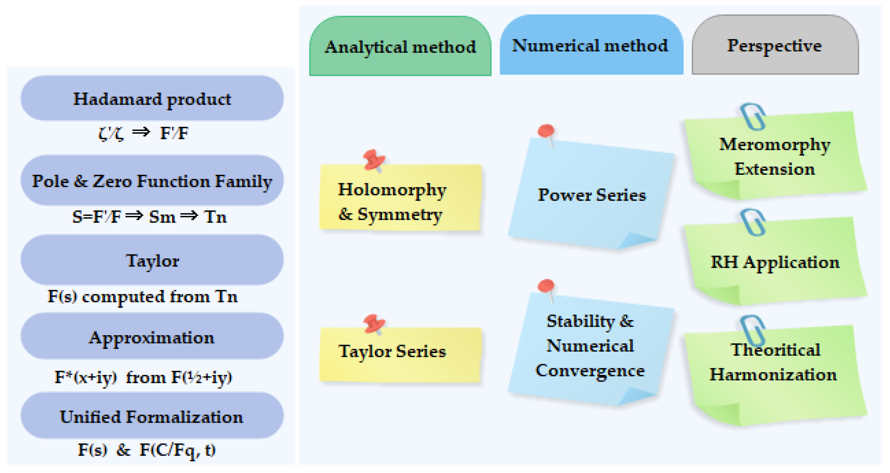
2. Materials and Methods

2.1. Mathematical Notations

Where possible, classical mathematical notations have been selected (Table 1): to lighten the writing, some original notations are defined.

Table 1. Notations.

Definition	Notation
Absolute value	$\forall a∊ℝ: \left|a\right|=a if a>0;-a if a<0$
Complex number	$\forall z\in ℂ:z=x+iy=r{e}^{i\theta }=\left|z\right|e^{i arg\left(z\right)}$ $\left|z\right|=\left|x+iy\right|=\sqrt{x^2+y^2} ;x,y, r, \theta \in ℝ$
Integer and fractional parts	In $ℝ$, the integer part and the fractional part of a real number $a$: $\forall a∊ℝ:a=\left[a\right]+\left\{a\right\}; \left[a\right]∊\mathbb{N}, 0\le \left\{a\right\}<1$
Complex number in the CS	In $ℂ$, $s=x+i y=\Re \left(s\right)+i \Im \left(s\right);s\in ℂ;x, y ∊ ℝ;$ its conjugate $\overline{s}=x-i y$
Complex number $1-s$ associated with $s$	In $ℂ$, $\widehat{s}=1-s=1-x-i y;x, y ∊ ℝ;$ its conjugate $\check{s}=\overline{1-s}=\overline{\widehat{s}}=1-x+i y$ $\widehat{s}$ symmetric of $s$ with respect to ($½,0$)
Critical strip (CS)	In the CS $\mathcal{S}$: $s=\Re \left(s\right)+i \Im \left(s\right)=x+i y; 0\le x\le 1, y>0; s\ne 1$
Critical line (CL)	On the CL $ℒ:=x=\text{½}$: $𝓈=\text{½}+i𝓎; 𝓎>0$
CS, except the CL	$\mathcal{S}\backslash ℒ:=0\le x\le 1;x\ne \text{½}; \dot{x}=x-\text{½}; s\ne 1$
Zeta function: $\zeta$	$\zeta \left(s\right)={\displaystyle \sum }_1^{\infty }{n}^{-s}.$ In the CS, the $\zeta$ function is divergent. One considers in this CS, the analytical continuation $\eta \left(s\right)$.
Eta Dirichlet function: $\eta$	$\eta \left(s\right)=\zeta \left(s\right)\left(1-2^{-s+1}\right)$
Derivative of the $\zeta$ function	${\zeta }^{\prime }\left(s\right)={\displaystyle \sum }_{n=1}^{\infty }{n}^{-s}\log \left(n\right)$
Functional equation of the $\zeta$ function	$ℱℰ : \zeta \left(s\right)=\xi \left(s\right)\zeta \left(\widehat{s}\right)=\xi \left(s\right)\zeta \left(1-s\right)$ $\xi \left(s\right)=2^s{\pi }^{s-1}\sin \left(\pi s/2\right)\mathsf{\Gamma }\left(1-s\right)={\pi }^{s-\text{½}}\mathsf{\Gamma }\left(\widehat{s}/2\right)/\mathsf{\Gamma }\left(s/2\right)$
Functional equation on the CL	$ℱℰ : \zeta (𝓈)=\xi (𝓈)\zeta \left(\widehat{𝓈}\right)=\xi (𝓈)\zeta \left(\overline{𝓈}\right)=\xi (𝓈)\overline{\zeta }(𝓈)$ $\xi (𝓈)={\pi }^{i𝓎}\overline{\mathsf{\Gamma }}\left(𝓈/2\right)/\mathsf{\Gamma }\left(𝓈/2\right)$
Anamorphosis	$\tilde{y}=y/\left(2\pi \right)\ln \left(y/\left(2\pi e\right)\right).$ The anamorphosis produces a stronger elongation of the $y$ axis as $y$ increases.
Zeros $ℨ$ in the CS\CL	$s_q\in \mathcal{S}\backslash ℒ: s_q=x_q+i y_q; \zeta \left(s_q\right)=0$
Zeros $\mathcal{Z}$ on the CL	${𝓈}_p\in ℒ\subset \mathcal{S}: {𝓈}_p=\text{½}+i {𝓎}_p; \zeta \left({𝓈}_p\right)=0$ The zeros are ordered in pairs, $s$ and $\widehat{s}=1-s$ Calculations are carried out with $y>0$
Lambert function	The main branch is defined by: $W\left(z\right)=w \iff z=w{e}^w;z\ge -1/e$
Gamma function	$\mathsf{\Gamma }\left(z\right)={{\displaystyle \int }}_0^{\infty }{t}^{z-1}{e}^{-t}dt$
Lower incomplete Gamma function	$\mathsf{\gamma }\left(z,a\right)={{\displaystyle \int }}_0^{\mathrm{a}}{t}^{z-1}{e}^{-t}dt=a^z{e}^{-a}{\displaystyle \sum }_0^{\infty }\frac{\mathsf{\Gamma }\left(z\right)a^k}{\mathsf{\Gamma }\left(z+k+1\right)}$
Digamma function	${\psi }_0\left(z\right)={\mathsf{\Gamma }}^{\prime }\left(z\right)/\mathsf{\Gamma }\left(z\right)$
Jacobi function	$\vartheta \left(z;\tau \right)={\displaystyle {\displaystyle \sum }_{n\in \mathbb{Z}}}{e}^{i\pi \left(n^2\tau +2nz\right)}$
Pochhammer symbol	Rising factorial: ${\left(x\right)}_n=x\left(x+1\right)\dots \left(x+n-1\right)={\displaystyle \prod }_{k=1}^n\left(x+k-1\right)$
Euler’s constant	Euler–Mascheroni constant: $\gamma =\underset{n\to \infty }{\lim }\left(-\ln n+{\displaystyle \sum }_{k=1}^n\frac{1}{k}\right)\approx 0.5772156649$
Taylor series	$f\left(z\right)={\displaystyle \sum }_{n=0}^{\infty }\frac{f^{\left(n\right)}\left(a\right)}{n!}{\left(z-a\right)}^n$
Bernoulli numbers	Coefficients of the power series of $\frac{t}{e^t-1}={\displaystyle \sum }_{n=0}^{\infty }{ℬ}_n\frac{t^n}{n!}$ $$\begin{gathered} {ℬ}_0=1; {ℬ}_1=-\text{½}; if k>0:{ℬ}_{2k+1}=0 ;{ℬ}_2=\frac{1}{6};{ℬ}_4=-\frac{1}{30};{ℬ}_6=\frac{1}{42}; \\ {ℬ}_8=-\frac{1}{30};{ℬ}_{10}=\frac{5}{66};{ℬ}_{12}=-\frac{691}{2730};{ℬ}_{14}=\frac{7}{6};{ℬ}_{16}=-\frac{3617}{510};{ℬ}_{18}=\frac{43867}{798}; \end{gathered}$$ ${ℬ}_{2n}={\left(-1\right)}^{n-1}\left|{ℬ}_{2n}\right|$; ${ℬ}_{2n}~{\left(-1\right)}^{n-1}\frac{2\left(2n\right)!}{{\left(2\pi \right)}^{2n}}$

2.2. Complex Analysis Reminders

2.2.1. Holomorphic and Meromorphic Functions

A holomorphic function is a complex differentiable function, which is complex differentiable everywhere within some open disk centered at each point $z$ in a domain in the complex plane $ℂ$. The existence of a complex derivative in a neighborhood implies that a holomorphic function is infinitely differentiable and locally equal to its own Taylor series. A holomorphic function whose domain is the whole complex plane is called an entire function. Any holomorphic function has an expansion as a power series. Holomorphic functions are conformal: they preserve angles between curves. Complex derivatives act infinitesimally by rescaling and rotating (multiplication by a complex number).

A holomorphic function, having only isolated singularities which are poles, is called a meromorphic function. Let $\mathcal{D}$ be an open connected subset of $ℂ$. A function $f$ is meromorphic on $\mathcal{D}$ if for all $z\in \mathcal{D}$ there is $r>0$ such that either $f$ is holomorphic in $B\left(z,r\right)$ (the open ball of center $z$ and radius $r$) or $f$ is holomorphic in $\dot{B}=B\left(z_0,r\right)-\left\{z_0\right\}$, undefined in $z_0$ but there exists a positive integer $m$ such that:

$$\underset{z\to z_0}{lim}{\left(z-z_0\right)}^{m}f\left(z\right)=c$$

$m_0$ is the least of such integers $m$ satisfying the limit. If $m_0=1$ then $z_0$ is a removable singularity (e.g., $\sin z/z; z_0=0$). If $m_0\ge 2$ then $z_0$ is a pole. If an isolated singularity is neither removable nor a pole, it is said to be essential (e.g., $e^{1/z}; z_0=0$).

Any meromorphic function in $ℂ$ is the ratio of two entire functions.

2.2.2. Weierstraß’s and Hadamard’s Factorization Theorems

Weierstraß’s theorem states that every entire function can be represented by a possibly infinite product, called the Weierstraß product, involving their zeros [19].

A family of parts of a topological space is said to be locally finite when each point has a neighborhood which meets only a finite number of elements of the family. Let $\mathcal{D}$ be a locally finite set in $ℂ$, divided into two disjoint parts $\mathcal{𝒫}$ and $\mathcal{Z}$. We attach to any point of $\mathcal{D}$ a positive integer $\omega \left(z\right)$. Then, there exists a meromorphic function $f$ on $ℂ$ such that $\mathcal{𝒫}$ is the set of poles of $f$. $\mathcal{Z}$ is the set of zeros in $F$, for all points within $\mathcal{D}$ $\left(\forall z\in \mathcal{D}\right)$, $\omega \left(z\right)$ is the order of the pole or zero $z$.

Theorem 1 

(Weierstraß’s factorization). The primary factors are $E_0\left(z\right)=\left(1-z\right)$ and $E_n\left(z\right)=\left(1-z\right) exp\left({\displaystyle \sum }_{k=1}^n{z}^k/k\right)$. $f$ is an entire function, which has a zero at $z=0$ of order $m\ge 0$ and $\left\{a_k\right\}$ are the other zeros repeated according to multiplicity $\mathsf{\omega }\left(k\right)$ . There exists an entire function $g$ and a sequence of integers $\left\{p_k\right\}$ such that:

$$f\left(z\right)=z^m{e}^{g\left(z\right)}P\left(z\right);P\left(z\right)={{\displaystyle \prod }}_{k=1}^{\infty }{E}_{p_k}\left(z/a_k\right)$$

Theorem 2 

(Hadamard’s factorization). If $f$ is an entire function of finite order $\rho$ and $m$ is the order of the zero of $f$ at $z=0$, then $f\left(z\right)=z^m{e}^{g\left(z\right)}P\left(z\right)$,

$$P\left(z\right)={{\displaystyle \prod }}_{k=1}^{\infty }{E}_p\left(\frac{z}{a_k}\right)={{\displaystyle \prod }}_{k=1}^{\infty }\left(1-\frac{z}{a_k}\right)e^{q_k\left(z\right)};{ q}_k\left(z\right)=\frac{z}{a_k}+\frac{1}{2}{\left(\frac{z}{a_k}\right)}^2+\cdots +\frac{1}{p_k}{\left(\frac{z}{a_k}\right)}^{p_k}.$$

$g\left(z\right)$ is a polynomial of degree $q\le \rho$ and $p=\left[\rho \right]$. $g\left(z\right)$ and each $q_k\left(z\right)$ are polynomials of degree $\le h$, $h$ , the smallest number, is the genus of $f\left(z\right)$. $P\left(z\right)$ is the canonical product.

2.3. Reminders on Special Functions

In this paragraph, we recall the classic formulas used in the article.

2.3.1. The Gamma Function

The Gamma function is defined as the analytic continuation of the following integral function to a meromorphic function that is holomorphic in the whole complex plane except zero and the negative integers, where the function has simple poles:

$$\Gamma \left(z\right)={{\displaystyle \int }}_0^{\infty }{t}^{z-1}{e}^{-t}dt; ℱℰ : \Gamma \left(z+1\right)=z\Gamma \left(z\right); \Gamma \left(\overline{z}\right)=\overline{\Gamma }\left(z\right)$$

Power series of the Gamma function:

$$\forall z\in ℂ: \Gamma \left(z\right)={{\displaystyle \int }}_0^{\infty }{u}^z{e}^{-u}\frac{du}{u}=\sqrt{2\pi }{z}^{z-½}{e}^{-z+\mu \left(z\right)}; \mu \left(z\right)={{\displaystyle \sum }}_{k=1}^{\infty }\frac{B_{2k}}{2k\left(2k-1\right)z^{2k-1}}$$

(2)

Euler’s reflection formula and Legendre’s duplication formula:

$$\begin{gathered} \forall \mathrm{z}\notin \mathbb{Z}: \mathsf{\Gamma }\left(1-\mathrm{z}\right)\mathsf{\Gamma }\left(\mathrm{z}\right)= \mathsf{\pi }/\sin \mathsf{\pi }\mathrm{z} \\ \mathsf{\Gamma }\left(\mathrm{z}\right)\mathsf{\Gamma }\left(\mathrm{z}+\text{½}\right)=2^{1-2\mathrm{z}}\sqrt{\mathsf{\pi }}\mathsf{\Gamma }\left(2\mathrm{z}\right) \end{gathered}$$

(3)

2.3.2. The Incomplete Gamma Function

The lower and upper incomplete gamma function are defined as:

$$lower: \gamma \left(z, a\right)={{\displaystyle \int }}_0^a{t}^{z-1}{e}^{-t}dt; \forall \Re \left(z\right)>0; a\ge 0$$

$$upper: \Gamma \left(z, a\right)={{\displaystyle \int }}_a^{\infty }{t}^{z-1}{e}^{-t}dt; \forall z\in ℂ; a\ge 0$$

$$\Gamma \left(z\right)=\gamma \left(z, a\right)+\Gamma \left(z, a\right)$$

2.3.3. The Digamma Function

Definition, power series and Bohr–Mollerup’s $ℱℰ$:

$$\begin{gathered} {\mathsf{\psi }}_0\left(\mathrm{z}\right)= {\mathsf{\Gamma }}^{\prime }\left(\mathrm{z}\right)/\mathsf{\Gamma }\left(\mathrm{z}\right) \\ {\mathsf{\psi }}_0\left(\mathrm{z}\right)={\mathsf{\psi }}_0\left(1\right)-\frac{1}{\mathrm{z}}+\mathrm{z}{{\displaystyle \sum }}_{\mathrm{k}=1}^{\infty }\frac{1}{\mathrm{k}\left(\mathrm{k}+\mathrm{z}\right)};{ \mathsf{\psi }}_0\left(1\right)=-\mathsf{\gamma } \\ {\mathsf{\psi }}_0\left(1+\mathrm{z}\right)={\mathsf{\psi }}_0\left(\mathrm{z}\right)+1/\mathrm{z} \end{gathered}$$

(4)

2.3.4. The Zeta ($\zeta$) Function

The Riemann zeta function, ζ(s), is a mathematical function of a complex variable s, and can be expressed as:

$$\forall s\in ℂ,s\ne 1:\zeta \left(s\right)={{\displaystyle \sum }}_{n=1}^{\infty }{n}^{-s}$$

The function is divergent in the CS $\mathcal{S}$. The analytical extension is Dirichlet’s eta function: $\eta \left(s\right)=\zeta \left(s\right)\left(1-2^{-s+1}\right)$.

The $ℱℰ$ of the $\zeta$ function is defined by:

$$\forall s\in ℂ;s\ne 0;s\ne 1:\zeta \left(s\right)=2^s{\pi }^{s-1}sin\left(\pi s/2\right)\Gamma \left(1-s\right)\zeta \left(1-s\right)$$

(5)

The $n$ non-trivial zeros on the CL and potentially in the CS are $\zeta \left(z_n\right)=\zeta \left({\widehat{z}}_n\right)=0$.

The expression of the Hadamard product for the $\zeta$ function is:

$$\zeta \left(s\right)=\frac{e^{\left(ln\left(2\pi \right)-1-\frac{\gamma }{2}\right)s}}{2\left(s-1\right)\Gamma \left(1+\frac{s}{2}\right)}{{\displaystyle \prod }}_{\rho }\left(1-\frac{s}{\rho }\right)e^{s/\rho };\forall \rho :\zeta \left(\rho \right)=0$$

From this Hadamard product, we deduce the expression:

$$\frac{{\zeta }^{\prime }\left(s\right)}{\zeta \left(s\right)}=ln2\pi -1-\frac{\gamma }{2}-\frac{1}{s-1}-\frac{1}{2}\frac{{\Gamma }^{\prime }\left(1+s/2\right)}{\Gamma \left(1+s/2\right)}+{\displaystyle \sum }_{\rho }\left(\frac{1}{s-\rho }+\frac{1}{\rho }\right)$$

(6)

The sum is over the non-trivial zeros $\rho$ of the $\zeta$ function and $\gamma$ is the Euler–Mascheroni constant.

$$s=0: \zeta \left(0\right)=-½; {\zeta }^{\prime }\left(0\right)=-½ln2\pi ; \frac{{\zeta }^{\prime }\left(0\right)}{\zeta \left(0\right)}=ln2\pi$$

Moreover, B. Riemann was familiar with the expression:

$${\displaystyle \sum }_{\rho }\frac{1}{\rho }=1+\frac{1}{2}\gamma -ln2-\frac{1}{2}ln\pi$$

(7)

$F$ is also expressed with the Jacobi–Euler function:

$$F\left(s\right)={{\displaystyle \int }}_0^{\infty }\frac{\vartheta \left(0;iu\right)-1}{2}{u}^{s/2}\frac{du}{u}$$

2.4. RH over a Finite Field

We know how to prove the RH for the $\zeta$ functions of curves over finite fields. The RH analogy between the number field and finite fields was initialized by E Artin [20] and demonstrated by Hasse [21,22] for curves of genus 1. The $\zeta$ function, the $ℱℰ$ and the RH can be formulated for congruences on these geometric structures. It is then a matter of finding the number of rational points on a curve, when we endow the set of points of the plane algebraic curve with a finite field structure ${\mathbb{F}}_q;q=p^f; \mathbb{Z}/p\mathbb{Z};p prime$. In 1949, Weil [23] published the conjectures on non-singular projective manifolds of dimension $N$, demonstrated by Deligne [24,25] in 1973. The version for curves ($N=1$), is as follows:

Theorem 3 

(Deligne’s). Let $\mathcal{C}/{\mathbb{F}}_q$ be a complete non-singular curve of genus $g$ over ${\mathbb{F}}_q$.

The $\zeta$ function is a rational fraction: $Z\left(\mathcal{C}/{\mathbb{F}}_q,t\right)\in \mathbb{Q}\left(t\right); t=q^{-s}$

$$Z\left(\mathcal{C}/{\mathbb{F}}_q,t\right)=\frac{f\left(t\right)}{\left(1-t\right)\left(1-qt\right)}=\frac{{{\displaystyle \prod }}_{j=1}^{2g}\left(1-{\omega }_{j}t\right)}{\left(1-t\right)\left(1-qt\right)}$$

$f\left(t\right)\in {\mathbb{Z}}_{2g}\left[t\right]$ is a polynomial of degree $2g$ , with integer coefficients. $\zeta$ has a single pole at $t=1$ , with residue $h/\left(q-1\right)$; $h$ is the number of classes.

The $ℱℰ$ is: $Z\left(\mathcal{C},1/qt\right)={\left({qt}^2\right)}^{1-g}Z\left(\mathcal{C},t\right)$

The zeros of the $\zeta$ function are the inverses of ${\omega }_j$. The RH holds:

$$\Re \left({\omega }_j{}^{-1}\right)=\text{½}; {{\displaystyle \prod }}_{j=1}^{2g}{\omega }_j=q^g; \forall j:\left|{\omega }_j\right|=\sqrt{q}$$

For a manifold of dimension $N$, the $\zeta$ function is factored into a polynomial $P_j\left(t\right)$ with integer coefficients.

$$Z\left(\mathcal{C}/{\mathbb{F}}_q,t\right)={{\displaystyle \prod }}_{j=1}^{2N-1}{P}_j/{{\displaystyle \prod }}_{j=0}^{2N}{P}_j$$

$$P_0\left(t\right)=1-t; P_{2N}\left(t\right)=1-q^{N}t;0<j<2N: P_j \left(t\right)={{\displaystyle \prod }}_{k=1}^{d_j}\left(1-{\omega }_{j,k}t\right)$$

${\omega }_{j,k}$ are algebraic integers: $\left|{\omega }_{j,k}\right|=\sqrt{q}$; $d_j$ are the degrees of the polynomials $P_j$.

2.5. Reasoning Strategy

We have published three graphical and numerical studies on the $\zeta$ function in the CS.

• In [26], we analyzed the genesis of the numerical value $\zeta \left(s\right)$ of the function from the original series, by identifying three phases, according to the development of the index n of the series; firstly, influential and constitutive phase of the value by successive plateaus from 1 to $n_1=\left[y/2\pi \right]$, secondly a phase completing the final value of $n_1+1$ to $n_2=\left[y/\pi \right]$, and finally a divergent phase without influence on the value $\zeta \left(s\right)$ of $n_2+1$ to infinity.
• In [27], we calculated the serial expansion of $\xi \left(s\right)=\zeta \left(s\right)/\zeta \left(1-s\right)$, in the CS, with its reduced transcription on the CL. From these formulas emerges a geometric interpretation of $\xi \left(s\right)$ in the group of similitudes, i.e., a homothety and four rotations, followed by a final transformation ε, which prefigures the RH.
• In [28], we proposed a two-layer stochastic model of the position of the nth zero on the CL, with its estimate of the ordinate $y_n=2\pi \frac{n-2+⅝}{W\left(\frac{n-2+⅝}{e}\right)}.$ The two layers are composed of one deterministic layer, via the Lambert function $W$. The second layer is stochastic via Gaussian random variables.

In this present article, we no longer focus on the $\zeta$ function alone, but we analyze it, through the prism of the envelope via the Jacobi theta function and Euler’s gamma function, which allows us to immediately incorporate its functional equation. This construction, as demonstrated by B. Riemann, makes it possible to materialize the properties of the $\zeta$ function. Following the work of Weierstraß, the Hadamard product formula then makes it possible to introduce the coordinates of the zeros into the formulas. We then obtain, by Taylor’s formula, a means of operationally calculating the values $F\left(s\right)$ in the CS. The calculations are laborious, especially since the convergence towards the value $F\left(s\right)$ is slow; it is necessary to inject knowledge of many coordinates of zeros close to $s=x+iy$ to achieve an accurate result. Convergence is assured and the error is in the order of $F^{\left(n\right)}\left(½+iy\right){\left(x-½\right)}^n/n!$, which depends on the number of terms in the Taylor series. The numerical computation thus leads to the following result, in the CS\CL ($x\ne ½$); the modulus $\left|F\left(s\right)\right|$ is never zero. Thanks to this function $F$; we also detect the seeds of the RH in the morphology of the function $F$, which consists of a foliation of elementary functions $F_k\left(s\right)={\left(s+2k\right)}^{-1}+{\left(1-s+2k\right)}^{-1},$ referred to here as Pochhammer surfaces. This accumulation of functions $F_k\left(s\right)$ is interpreted geometrically in 3D according to two surfaces; the imaginary component respects the nullity on the CL and the symmetry with respect to the line $x=½;z=0.$ The real component draws a corrugated sheet generally higher than the plane $z=0$, and symmetrical with respect to the $x=½$ plane. The zero-valued contours on the two surfaces do not meet in the CS\CL.

In this article, we use meromorphic functions (gamma, zeta, etc.). They are holomorphic functions except at isolated points. From these meromorphic functions, we make a new specific function $S$ created from the poles and zeros of the function resulting from the $ℱℰ$. $S$ turns out to be equal to the logarithmic derivative of the function $F$. We observe that there is a notable difference between direct calculations from mathematical formulas and indirect calculations from numerical evaluations which involve sums of series of numbers which converge very slowly. As the functions are meromorphic, we know that they are smooth and vary little locally. This makes it possible to remove ambiguities when numerical ‘fairy chimneys’ (unexpectedly large values) appear. These artefacts arise from numerical computations of the type $a=\epsilon \times \left(1/{\epsilon }^{\prime }\right)\approx 0\times \infty$, because of the limited length of floating-point numbers.

To dissect the RH in the CS, it is necessary to inject the essential properties of the $\zeta$ function into the mathematical expressions used for power expansions and to numerically verify the formulas with precision. The two fundamental properties are:

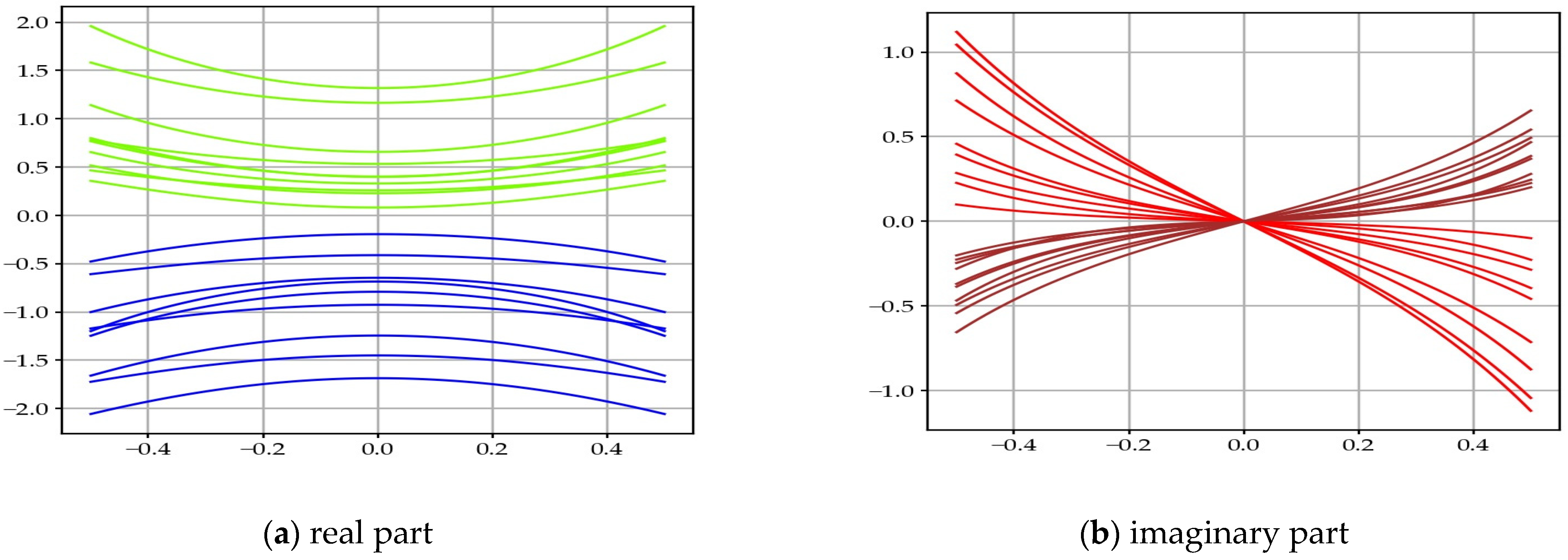
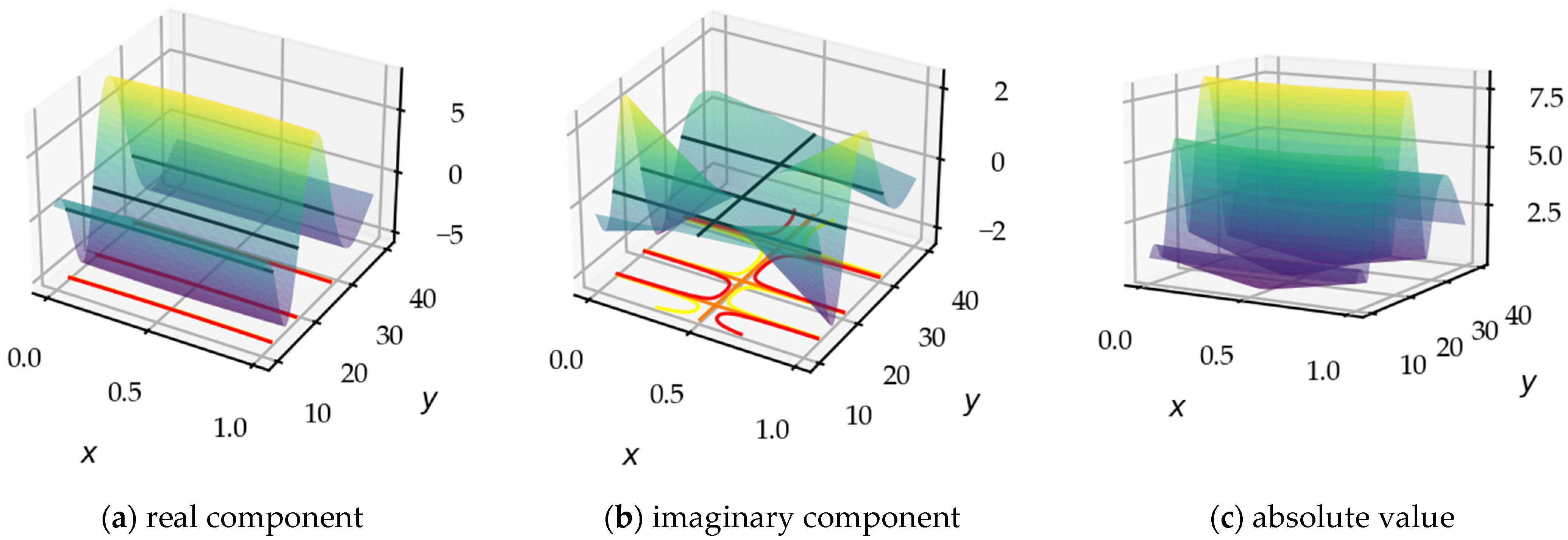
• Holomorphy: the $\zeta$ function is a continuous complex function, infinitely differentiable, and conformal, i.e., angles are preserved—the image of a circle is a circle.
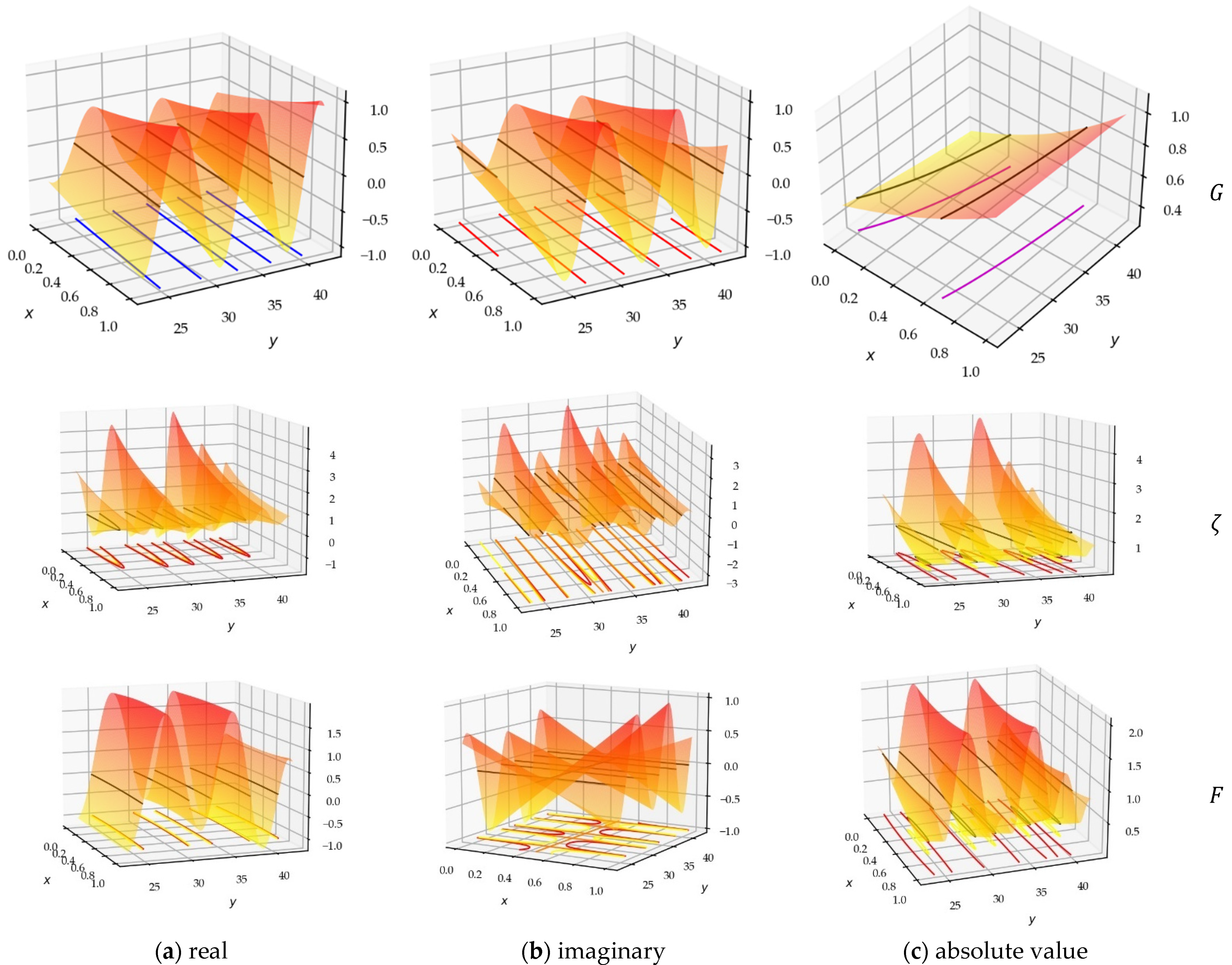
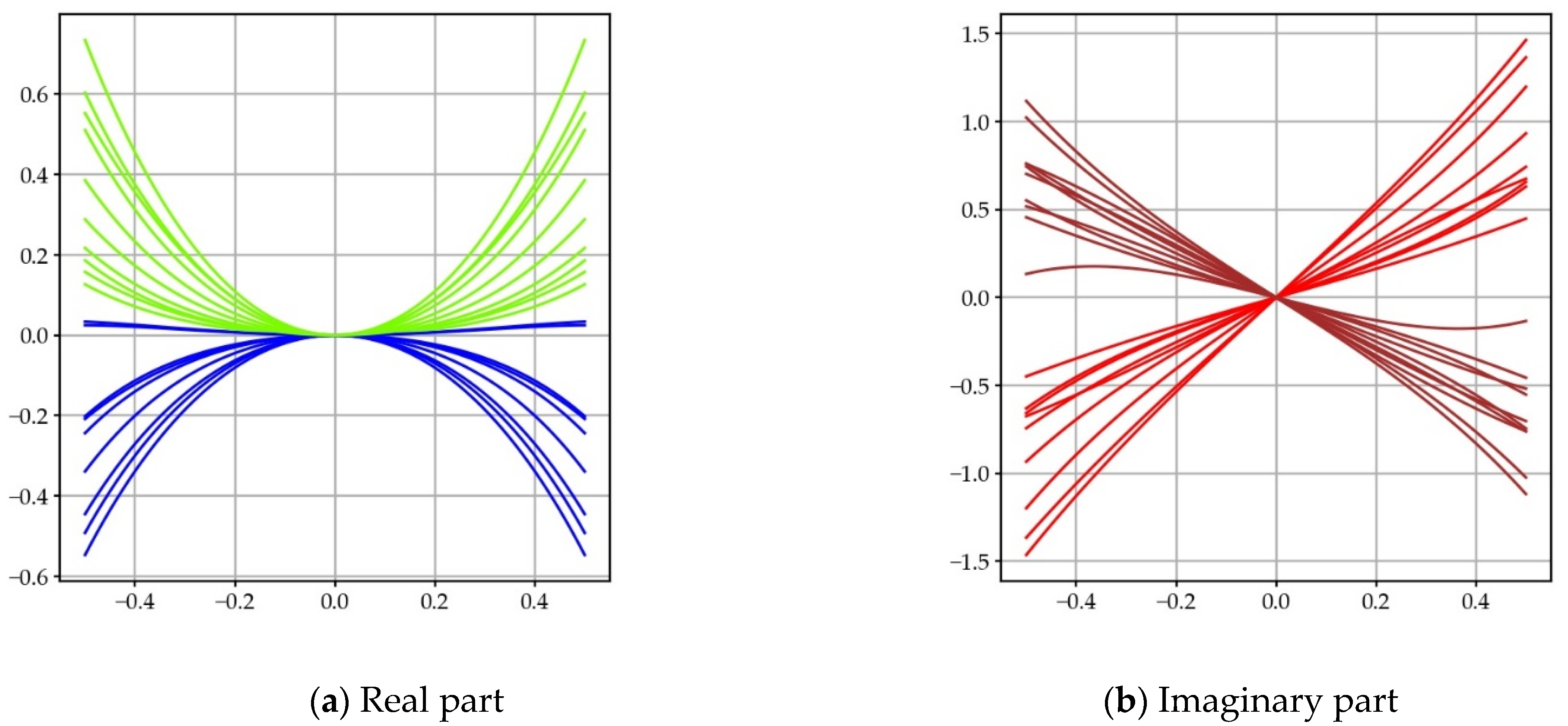
• The constitutional symmetry of the complex $ℱℰ$: the symmetry of the real surface with respect to the plane $x=½$ and the symmetry of the imaginary surface with respect to the line $z=0, x=½$.

These two properties, which account for the smooth local structure of the $\zeta$ function in the CS, are expressed in particular by the two formulas of the $ℱℰ$ and by the Taylor series expansion of the $F$ function. We will therefore apply the Taylor expansion of the holomorphic $F$ function which envelops the $\zeta$ function, and introduce the Hadamard product formula therein, in order to insert into the formula, the coordinates of the zeros of the $\zeta$ function. This construction allows the function to be calculated in two ways: directly by Taylor’s formula and indirectly with the information of known zeros. If we assume that $0<x<1\ll y$, we will thus be able to estimate the values $F\left(s\right)$ in the CS, from the values $F(𝓈)$ on the CL, being the line of symmetry. We can then evaluate and distinguish, in the CS, the two morphologies of the real and imaginary surfaces, along the $y$ axis, when $x=½$. For calculations, two cases arise, depending on whether the ordinate of $y$ is, or is not, that of a non-trivial zero. Table 2 shows the progression of the process, in Section 3 and Section 4 by highlighting the main milestones.

Table 2. Flowchart of the process with the main milestones.

Milestones	Analytical & Numerical
Riemann	$\zeta \left(s\right); F\left(s\right)=F\left(1-s\right)$
Zeros	$\zeta \left(s\right)=0 \iff F\left(s\right)=0$
Weierstraß, Hadamard	$\frac{{\zeta }^{\prime }}{\zeta }⇢\frac{F^{\prime }}{F}=S$
Poles and Zeros	$S={\displaystyle {\displaystyle \sum }_{poles}}\frac{1}{s-p_h}+{\displaystyle {\displaystyle \sum }_{zeros}}\frac{1}{s-z_n}$
$S, S_m,T_n$ Functions	$S⇢S_m⇢T_n$
Taylor	$F\left(s\right)=F(𝓈){\displaystyle {\displaystyle \sum }_{n\in \mathbb{N}}}\frac{{\left(\Delta s\right)}^n}{n!}{T}_n$
RH	$\left|F\left(s\right)\right|>\left|F(𝓈)\right|; F\left(s\right)=0 \iff \zeta \left(s\right)=0$
Congruence	$\tilde{y}=y/\left(2\pi \right)\ln \left(y/\left(2\pi e\right)\right); {\mathbb{F}}_q$
Meromorphy, Weierstraß	$\underset{z\to z_0}{\lim }{\left(z-z_0\right)}^{m}f\left(z\right)=c$
Infinite and Finite Fields	Primes $p\in \mathbb{N}$; $P\left(x,y\right)=0 on \mathcal{C}/{\mathbb{F}}_q$
Jacobi–Weierstraß Elliptics	$\vartheta \left(z;\tau \right)={\displaystyle {\displaystyle \sum }_{n\in \mathbb{Z}}}{e}^{i\pi \left(n^2\tau +2nz\right)}; F\left(s\right)={{\displaystyle \int }}_0^{\infty }\frac{\vartheta \left(0;iu\right)-1}{2}{u}^{s/2}\frac{du}{u}$

2.6. RH Analysis

To determine whether the RH is true, we will calculate, by a series expansion, the $F$ function of a point $Z\left(s=x+iy\right)$ of the CS, from a point $H\left(𝓈=\text{½}+iy\right)$ on the CL ($x$ is very small compared to $y$ on this line) which is located on the same $y$-ordinate. To achieve this progress, we will calculate the derivatives of $\zeta$, then the successive derivatives of $F\left(s\right)$. We will then calculate $F(𝓈)$ when the point $𝓈$ is on the CL. The numerical calculations are laborious.

During this power series analysis, a difficulty arises and this case must be handled separately. Indeed, the obstacle appears when $y$ is equal to $y_p$, where there is already a non-trivial zero on the CL.

3. Results

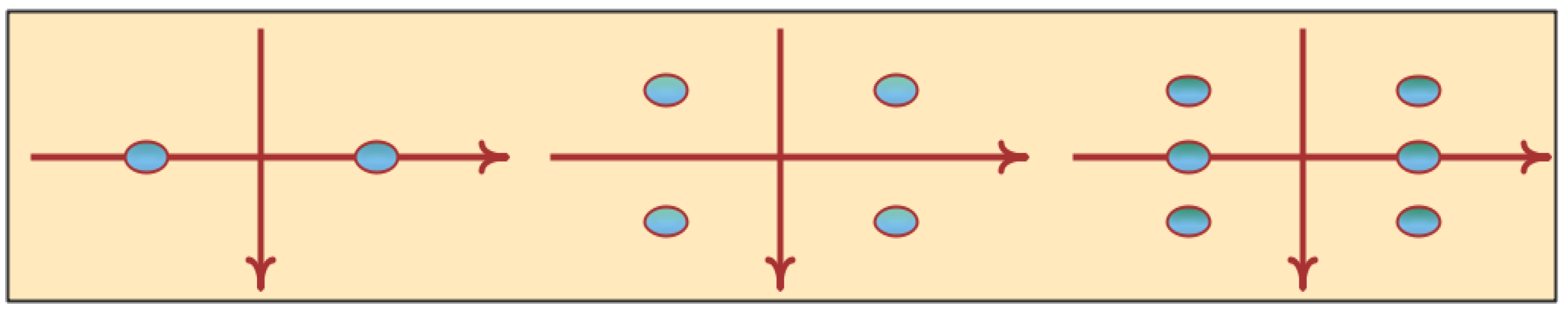
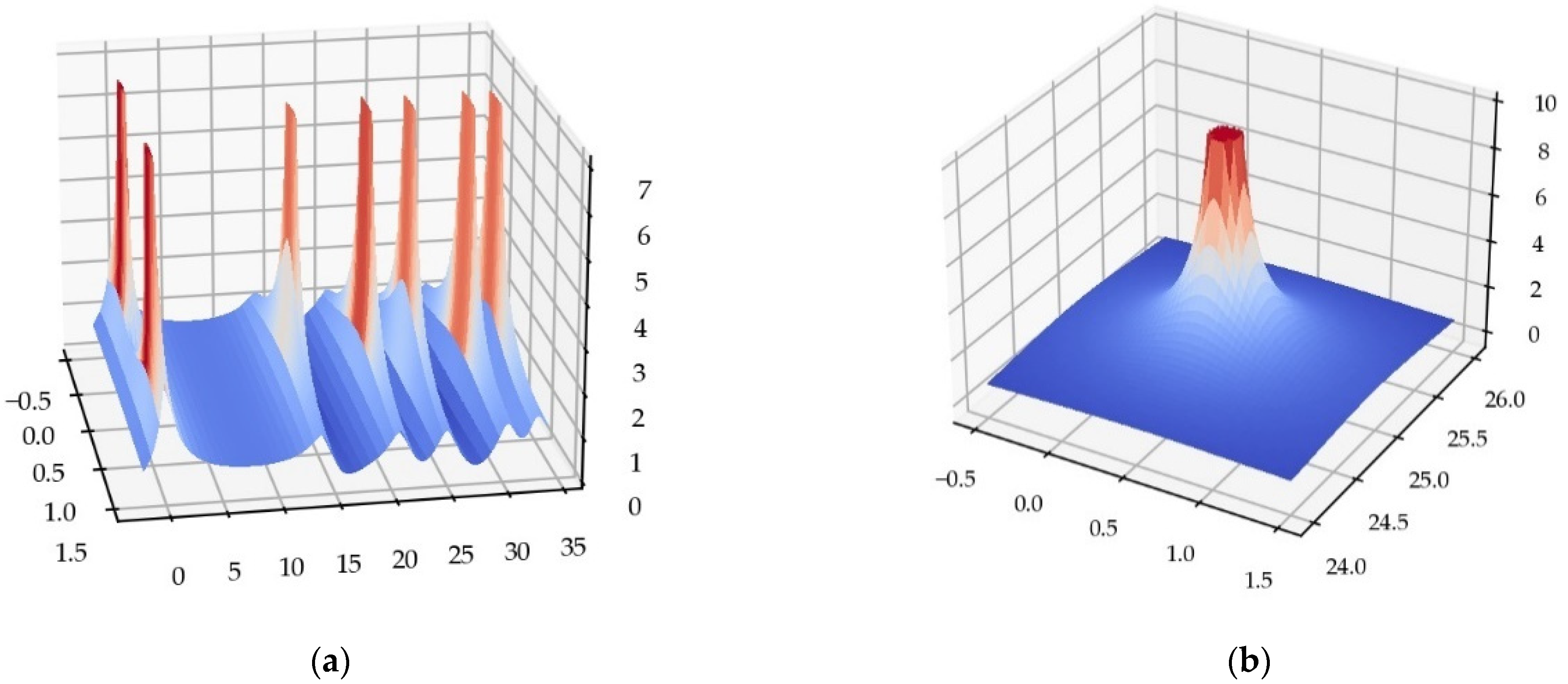
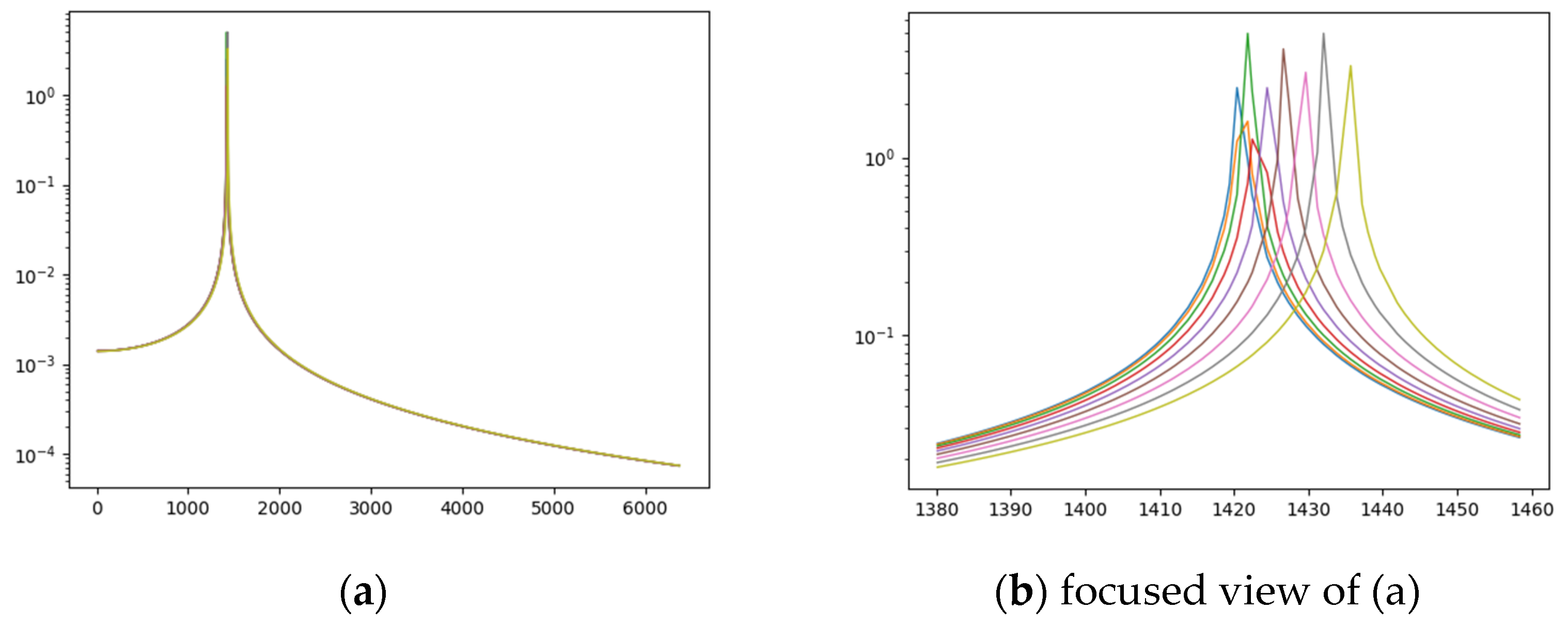
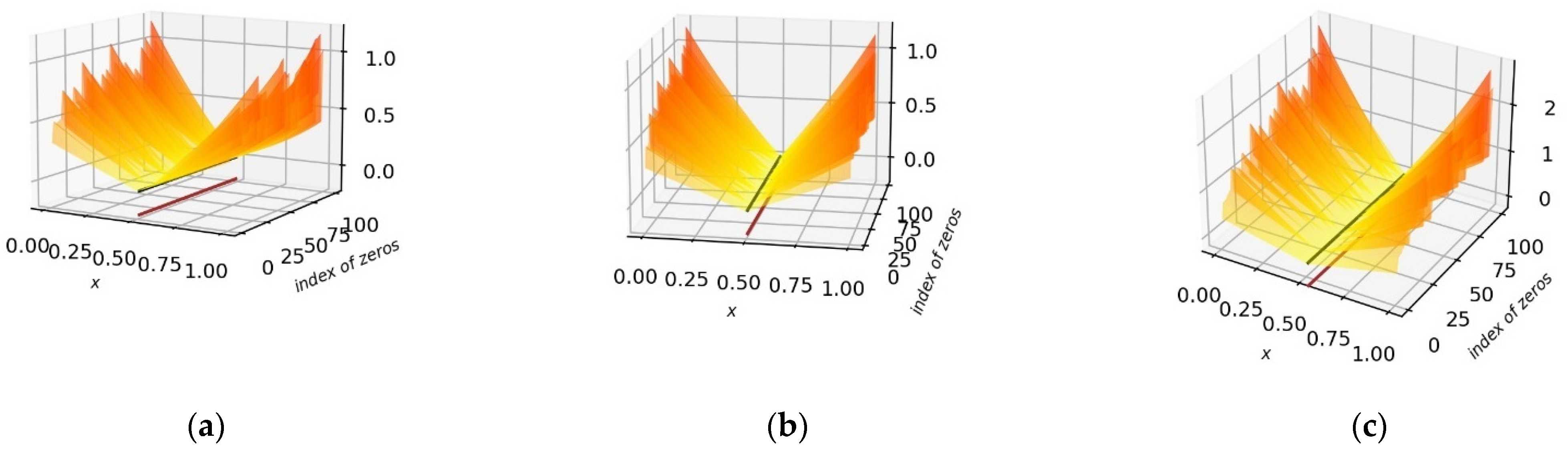
3.1. The Zeros of the $\mathsf{\zeta }$ Function

The non-trivial zeros of the $\zeta$ function are identified in pairs: $z_n=s_n=x_n+i{y}_n$ and ${\widehat{z}}_n={\widehat{s}}_n=1-s_n$. However, it is formally necessary to separate the two disjoint subsets $\mathcal{Z}$ and $ℨ$ of non-trivial zeros.

$$\mathcal{Z}\subset ℒ; \mathcal{Z}≔\left\{{𝓈}_p=\text{½}\pm {iy}_p;{𝓈}_p\in ℒ; \mathsf{\zeta }\left({𝓈}_p\right)=0; p\in \left\{\mathbb{N}{\displaystyle \cup }{\aleph }_0\right\}\right\}$$

$$ℨ\subset \mathcal{S}\backslash ℒ;ℨ≔\left\{x_q\ne \text{½};{ s}_q=x_q\pm {iy}_q;{\widehat{s}}_q=1-s_q=1-x_q\mp {iy}_q; \mathsf{\zeta }\left(s_q\right)=\mathsf{\zeta }\left({\widehat{s}}_q\right)=0;q\in \left[0,Q\right];Q\in \left\{\mathbb{N}{\displaystyle \cup }{\aleph }_0\right\}\right\}$$

$Q$ is the number of possible zeros in the CS, excluding the CL: it is either infinite, or a non-negative integer: $Q\in \left\{0, 1,\dots , n,\dots ,\infty \right\}.$ The number of zeros $\#\left(\mathcal{Z}{\displaystyle \cup }ℨ\right)=P+Q$ is infinite, and the fertile region of these zeros remains fuzzy, even if we know that it is included in the CS $\mathcal{S}$ and that it necessarily includes the CL $ℒ$. Apart from the trivial zeros (the even negative integers of $\mathbb{Z}$), there are hypothetically three kinds of non-trivial zeros (Figure 1):

Figure 1. The three scenarios: illustrations of the subsets of zeros, in pairs, quadruplets, and sextuplets.

(1)

The zeros ${𝓈}_p=½\pm i{y}_p$ are on the CL $ℒ$. They are isolated points. We are certain that there exist $P={\aleph }_0$ of them.

(2)

The zeros $s_q=x_q+i{y}_q$ in the CS $\mathcal{S}\backslash ℒ$. In this case, the zeros come in quadruplets: $s_q, {\widehat{s}}_q=1-s_q, {\overline{s}}_q,1-{\overline{s}}_q$. Their cardinality $Q\in \left\{0, 1,\dots ,{\aleph }_0\right\}$ is unknown. The RH refutes their existence ($Q=0$).

(3)

A teratological case must be considered: zeros of the CL are aligned with zeros in the CS. In this case, there are six zeros, which are the combination of the two previous cases.

3.2. The Power Series of the Gamma Function $G\left(s\right)=\Gamma \left(s/2\right)/{\pi }^{s/2}$

The gamma function uses extremely low numerical values in the CS which vary immeasurably exponentially (Table 3):

Table 3. Regularization of the gamma function to restrict the spectrum of values.

$\mathit{n}$	$\mathit{y}={10}^{\mathit{n}}$	$\mathbf{\Gamma }\left(\left(½+\mathit{i}\mathit{y}\right)/2\right)$	${\mathit{e}}^{\frac{\mathit{\pi }\mathit{y}}{4}}\mathbf{\Gamma }\left(\left(½+\mathit{i}\mathit{y}\right)/2\right)/{\mathit{\pi }}^{\left(½+\mathit{i}\mathit{y}\right)/2}$
$1$	$10$	$-0.000 575 868+i 0.000 303 485$	$-1.255 999 9-i 0.093 768 6$
$2$	$100$	${10}^{-35}\times \left(5.625 84+i 4.694 49\right)$	$0.708 025+i 0.005 360 51$
$3$	$1000$	${10}^{-342}\times \left(3.497 24-i 2.447 05\right)$	$0.142 192-i 0.371 906$
$4$	${10}^4$	${10}^{-3 412}\times \left(3.088 42-i 1.458 68\right)$	$0.222 578-i 0.024 326 4$
$5$	${10}^5$	${10}^{-34,112}\times \left(-0.082 806 6+i 65.388 4\right)$	$0.022 978 7-i 0.123 795$
$6$	${10}^6$	${10}^{-341,096}\times \left(7.495 97-i 1.713 42\right)$	$-0.001 919 88+i 0.070 778 3$
$7$	${10}^7$	${10}^{-3,410,943}\times \left(2.051 78+i 6.602 77\right)$	$0.031 786 4+i 0.023 978 2$
$8$	${10}^8$	${10}^{-34,109,411}\times \left(-3.998 17-i 1.438 71\right)$	$-0.020 654 8-i 0.008 643 31$
$9$	${10}^9$	${10}^{-341,094,091}\times \left(2.864 07-i 5.050 57\right)$	$0.010 761 3-i 0.006 536 55$

To restrict the spectrum of values to a tighter interval and display the local variations of the gamma function, we compute a multiplicative factor which regularizes the function. We first decompose the gamma function in series, to know its expansion in $y$, using Formula (2). In the CS $\mathcal{S}$, we assume that $x$ is small relative to $y$. The function $G\left(s\right)$ of $F\left(s\right)=G\left(s\right)\times \zeta \left(s\right)$ becomes:

$$x\ll y; s=x+iy=iy\left(1-ix/y\right)$$

$$G\left(s\right)=\Gamma \left(s/2\right){\pi }^{-s/2}=\sqrt{2/e}{\left(s/2\pi e\right)}^{\frac{s-1}{2}}{e}^{\mu \left(s/2\right)}=\sqrt{2/e}{\left(iy\left(1-ix/y\right)/2\pi e\right)}^{\frac{s-1}{2}}{e}^{\mu \left(s/2\right)}$$

By decomposing into series, the expression ${\left(1-\mathrm{ix}/\mathrm{y}\right)}^{\frac{s-1}{2}}$, we detect the series $e^{\frac{x}{2}}$ which can be extracted and factored:

$${\left(1-ix/y\right)}^{\frac{s-1}{2}}=e^{\frac{x}{2}} 𝒫\left(x,y\right)=e^{\frac{x}{2}}\left(1+\frac{ix}{2y}{p}_1\left(x\right)+\frac{1}{2!}{\left(\frac{x}{2y}\right)}^2{p}_2\left(x\right)+\frac{i}{3!}{\left(\frac{x}{2y}\right)}^3{p}_3\left(x\right)+\frac{1}{4!}{\left(\frac{x}{2y}\right)}^4{p}_4\left(x\right)+\cdots \right)$$

We operate in the same way with the expression $e^{\mu \left(s/2\right)}$:

$$x\ll y; e^{\mu \left(s/2\right)}\cong \mathcal{Q}\left(x,y\right)=1+\frac{i{q}_1\left(x\right)}{6y}+\frac{q_2\left(x\right)}{6y^2}+\frac{i{q}_3\left(x\right)}{6y^3}+\frac{q_4\left(x\right)}{6y^4}+\dots$$

It then follows that:

$$G\left(s\right)=\sqrt{2/e} e^{i\frac{\pi }{4}\left(s-1\right)}{\left(y/2\pi e\right)}^{\frac{s-1}{2}}{e}^{\frac{x}{2}} 𝒫\left(x,y\right)\mathcal{Q}\left(x,y\right)$$

$$ℛ\left(x,y\right)=𝒫\left(x,y\right)\mathcal{Q}\left(x,y\right)=1+i\frac{r_1\left(x\right)}{12y}+\frac{r_2\left(x\right)}{2!\times {\left(12y\right)}^2}+i\frac{r_3\left(x\right)}{3!\times {\left(12y\right)}^3}+\frac{r_4\left(x\right)}{4!\times {\left(12y\right)}^4}+\dots$$

The end result is therefore:

$$G\left(s\right)=\sqrt{2} e^{\frac{-\pi y}{4}}{e}^{i\frac{\pi }{4}\left(x-1\right)+i\frac{y}{2}ln\frac{y}{2\pi e}} {\left(y/2\pi \right)}^{\frac{x-1}{2}}ℛ\left(x,y\right)$$

We define an angle $\phi$, a function of $x,y$ using the fractional part of the expression:

$$\phi =2\pi \left\{\frac{x-1}{8}+\frac{1}{2}\frac{y}{2\pi }ln\left(\frac{y}{2\pi e}\right)\right\}$$

$$G\left(s\right)=\Gamma \left(s/2\right){\pi }^{-s/2}=\sqrt{2} e^{\frac{-\pi y}{4}}{\left(y/2\pi \right)}^{\frac{x-1}{2}}ℛ\left(x,y\right) e^{i\phi }=M^{-1}{\left(y/2\pi \right)}^{\frac{x-1}{2}}ℛ\left(x,y\right) e^{i\phi }$$

The graphical multiplicative factor to visualize the function $F$ is therefore:

$$M={\left(\sqrt{2} e^{\frac{-\pi y}{4}}\right)}^{-1}=\sqrt{2}/2\times e^{\frac{\pi y}{4}}$$

(8)

In the rest of this article, all the graphs will be presented using this multiplying factor.

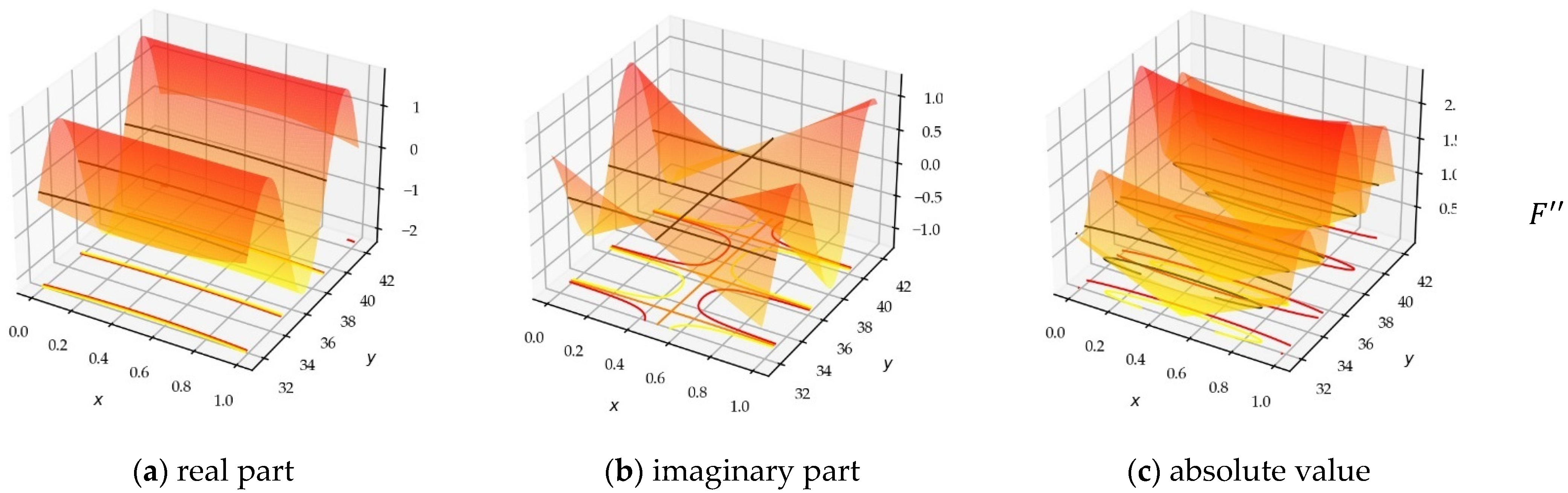
3.3. The $F$ Function from the $ℱℰ$

Using Formulas (5) and (3), the $ℱℰ$ of the $\zeta$ function can be defined by:

$$\forall s\in \mathcal{S}\subset ℂ≔\left\{0\le x\le 1;s\ne 0;s\ne 1\right\}; \widehat{s}=1-s: F\left(s\right)=\Gamma \left(s/2\right){\pi }^{-s/2}\zeta \left(s\right)=F\left(\widehat{s}\right)$$

(9)

The $\zeta$ function has only one pole ($p_1=1$), while the $F$ function has two ($p_0=s_0=0$ and $p_1={\widehat{s}}_0=1-s_0=1$). The frequency of the waves of the $F$ function is half that of the $\zeta$ function’s, due to the parameter $s/2$ (Figure 2).

Figure 2. Plots of $\zeta (𝓈)$ (blue and red) and $F(𝓈)$ (green & brown) on the CL $ℒ$ : $\Im \left(F\left(½+iy\right)\right)=0$. The frequency of the waves of the $F$ function is half that of the $\zeta$ function.

In Figure 3, we visualize the three surfaces, real and imaginary components and the absolute value, of the $\mathrm{G}, \zeta , F$ functions, with the multiplicative coefficient $e^{\pi y/4}/\sqrt{2}$ so as to erase the influence of the overall behavior of the gamma function. The 3D vision in the CS makes it possible to appreciate the properties of the surfaces and to distinguish the symmetries, and the zero contours. We can observe some characteristics and extract some properties: (i) The real surface $F$ is symmetrical with respect to the $x=½$ plane; (ii) The imaginary surface $F$ is symmetrical with respect to the line $z=0;x=½$.

Figure 3. (a) Real component; (b) imaginary component; (c) absolute value of the 3D Diagrams of the three functions $G$, $\zeta$, and $F$.

3.4. The Kernels of the $F$ and $\zeta$ Functions

The composition of $F$ shows that the kernels of $F$ and $\zeta$ are identical, since the $\mathsf{\Gamma }$ function and the exponential function $e^s$ never cancel each other out.

$$\begin{gathered} \forall s\in ℂ, s\ne \left\{0,-2k;k\in \mathbb{N}\right\}:\Gamma \left(s/2\right){\pi }^{-s/2} \not\equiv 0 \\ \forall s\in ℂ,s\ne \left\{0,1\right\}:F\left(s\right)=\Gamma \left(s/2\right){\pi }^{-s/2}\zeta \left(s\right)=F\left(1-s\right) \\ \forall s=x+iy\in \mathcal{S};0<x<1: \Gamma \left(s\right) \not\equiv 0;{ e}^s \not\equiv 0 \\ Kernel:=\left\{\forall s\in ℂ\backslash \left\{0,1,-2k | k\in \mathbb{N}\right\} | \zeta \left(s\right)=F\left(s\right)=0\right\} \\ \forall s\in ℂ\backslash \left\{0,1,-2k | k\in \mathbb{N}\right\}:Kernel≔ker\left(\zeta \right)\equiv ker\left(F\right) \\ \forall {𝓈}_p\in \mathcal{Z}\subset ℒ\subset \mathcal{S}\subset ℂ:\zeta \left({𝓈}_p\right)=0;\#\mathcal{Z}=P={\aleph }_0 \\ \forall s_q\in ℨ\subset \mathcal{S}\backslash ℒ\subset ℂ:\zeta \left(s_q\right)=0;\#ℨ=Q; Q\in \left\{0, 1,\dots , n,\dots ,\infty \right\} \end{gathered}$$

(10)

3.5. The Poles and Zeros $S$ Function

By combining Formulas (4), (6), and (7), we obtain a new formula. However, the logarithmic derivative of the $\zeta$ function is difficult to use because of its heterogeneity:

$${\zeta }^{\prime }\left(s\right)/\zeta \left(s\right)=½\left(ln\pi -{\psi }_0\left(s/2\right)\right)-(s^{-1}+{\left(s-1\right)}^{-1})+{{\displaystyle \sum }}_{n=1}^{\infty }{\left(s-z_n\right)}^{-1}$$

Using Formula (4), the power series of ${\psi }_0\left(s/2\right)$, this next formula has the advantage of highlighting the only pole, of value 1, the trivial zeros ($-2k$) and the non-trivial zeros $z_n$.

$$\frac{{\zeta }^{\prime }\left(s\right)}{\zeta \left(s\right)}=\frac{1}{2}\left(ln\pi +\gamma \right)-\frac{1}{s-1}-s{{\displaystyle \sum }}_{k=1}^{+\infty }\frac{1}{2k\left(2k+s\right)}+{\displaystyle \sum }_n\left(\frac{1}{s-z_n}\right)$$

The direct derivative of $\ln F\left(s\right)$ gives finally:

$$F\left(s\right)=\frac{\Gamma \left(s/2\right)}{{\pi }^{s/2}}\zeta \left(s\right)\Rightarrow \frac{d\left(lnF\left(s\right)\right)}{ds}=\frac{F^{\prime }\left(s\right)}{F\left(s\right)}=½{\psi }_0\left(s/2\right)-½ln\pi +\frac{{\zeta }^{\prime }\left(s\right)}{\zeta \left(s\right)}$$

$$F^{\prime }\left(s\right)/F\left(s\right)=-({\left(s-0\right)}^{-1}+{\left(s-1\right)}^{-1})+{{\displaystyle \sum }}_{n=1}^{\infty }{\left(s-z_n\right)}^{-1}$$

The logarithmic derivative of the $F$ function is in fact the poles and zeros function $S$ of this function (Figure 4), thus compatible with the canonical Weierstraß’s factorization.

$$\begin{gathered} \forall s\in ℂ; F\left(s\right)\ne 0: S\left(s\right)=\frac{d\left(lnF\left(s\right)\right)}{ds}=\frac{F^{\prime }\left(s\right)}{F\left(s\right)}=-{\displaystyle \sum }_{Poles}\frac{1}{s-p_h}+{\displaystyle \sum }_{Zeros}\frac{1}{s-z_n} \\ S\left(s\right)=-{\displaystyle \sum }_{Poles}\left(\frac{1}{s-p_h}+\frac{1}{s-{\widehat{p}}_h}\right)+{\displaystyle \sum }_{Zeros}\left(\frac{1}{s-z_n}+\frac{1}{s-{\widehat{z}}_n}\right) \end{gathered}$$

(11)

Figure 4. (a) The $S$ function: absolute value of $S\left(s\right)$, presenting the ‘fairy chimneys’ of the function, on the CL, and the two poles in the CS. (b) 3D view of a single pole. We only display the bottom of these very tall chimneys, since these pedestals are important for our study.

In the computation of the $S$ function, the non-trivial zeros must also be separated into those of the CL, which are in pairs, and those possibly outside the CL, which are in quadruplets.

$$\begin{gathered} \forall {𝓈}_p\in ℒ:\zeta \left({𝓈}_p\right)=0\Rightarrow \zeta \left({\overline{𝓈}}_p\right)=0 \\ \forall {𝓈}_q\in \mathcal{S}:\zeta \left(s_q\right)=0 \Rightarrow \zeta \left({\overline{s}}_q\right)=\zeta \left(1-s_q\right)=\zeta \left(1-{\overline{s}}_q\right)=0 \end{gathered}$$

The summation can therefore be broken down:

$${\displaystyle \sum }_{Zeros}\frac{1}{s-z_n}={\displaystyle \sum }_{Zeros \in ℒ}\frac{1}{s-{𝓈}_p}+{\displaystyle \sum }_{Zeros \in \mathcal{S}\backslash ℒ}\frac{1}{s-s_q}$$

$${\displaystyle \sum }_{Zeros}\frac{1}{s-z_n}={\displaystyle \sum }_{Zeros {𝓈}_p\in ℒ}\left(\frac{1}{s-{𝓈}_p}+\frac{1}{s-{\overline{𝓈}}_p}\right)+{\displaystyle \sum }_{Zeros s_q\in \mathcal{S}\backslash ℒ}\frac{1}{s-s_q}+\frac{1}{s-{\overline{s}}_q}+\frac{1}{s-\left(1-s_q\right)}+\frac{1}{s-\left(1-{\overline{s}}_q\right)}$$

The partial summation, when decomposed into a sum of two and a sum of four terms, shows that for a point $H$ of the CL $𝓈$, the total sum $S$ belongs to $iℝ$:

$$\forall 𝓈=\text{½}+iy\in ℒ:S(𝓈)=-2iyC;C\in ℝ$$

$$S(𝓈)=-\left(\frac{1}{𝓈}+\frac{1}{𝓈-1}\right)+{{\displaystyle \sum }}_{n=1}^{P+Q}\frac{1}{𝓈-s_n}=-2iyC$$

$$C=-\frac{1}{y^2+\mathrm{¼}}+{{\displaystyle \sum }}_{p=1}^P\frac{1}{y^2-y_p^2}+{{\displaystyle \sum }}_{q=1}^Q\frac{2\left(y^2+{\left(x_q-½\right)}^2-y_q{}^2\right)}{{\left(y^2+{\left(x_q-½\right)}^2+y_q{}^2\right)}^2-{\left(2y{y}_q\right)}^2}$$

A meromorphic function in $ℂ$ is represented by two surfaces, both smooth with a few isolated singularities. An associated function $S$, gathering all these points, and isolated points of zero value, in the form of a sum of rational fractions, appears as a ‘bed of nails’: with these nails pointing upwards from the zeros, and downwards from the poles. Despite the theoretical formulas being elementary, the numerical evaluation is more delicate in the neighborhoods of these singular points. The numerical computation of this $S$ function exhibits very slow convergence, whether or not one takes into account the RH. To reach three or four significant figures for the value of the function, it is advisable to take a very large number $\mathsf{𝕡}$ of zeros close to $s$ ($\mathsf{𝕡}>{10}^5$).

By observing Figure 5 (on the logarithmic scale on the ordinate), we understand that we can simplify the numerical calculation, by taking into account the exact value of the ordinates of the few thousand zeros close to $y$, and then considering an approximate value of millions of further zeros [28], taking ${\overline{y}}_p$ as the value of $y_p$. We can approximate further, by using $y_p\cong 2\pi \frac{p}{\ln p}$, as the influence of ${\left(y-y_p\right)}^{-1}$ is minimal when $y_p$ is far from $y$.

$$\mathrm{If} \left|y-y_p\right|>{10}^4, \mathrm{we} \mathrm{take} y_p\approx {\overline{y}}_p=2\pi \frac{p-2+⅝}{W\left(\frac{p-2+⅝}{e}\right)}. \mathrm{If} \left|y-y_p\right|>{10}^6, \mathrm{we} \mathrm{take} y_p\approx 2\pi \frac{p}{\ln p}.$$

$$\forall {\mathrm{y}}_{\mathrm{p}}\gg \mathrm{y}:{\mathrm{y}}_{\mathrm{p}}\approx 2\mathsf{\pi }\frac{\mathrm{p}}{\ln \mathrm{p}}\Rightarrow {{\displaystyle \sum }}_{\mathrm{p}=1}^{\infty }\frac{1}{{\mathrm{y}}^2-{\mathrm{y}}_{\mathrm{p}}{}^2}\approx {{\displaystyle \sum }}_{\mathrm{p}=1}^{\infty }\frac{1}{-{\mathrm{y}}_{\mathrm{p}}{}^2}\approx -{{\displaystyle \sum }}_{\mathrm{p}=1}^{\infty }\frac{1}{{\left(2\mathsf{\pi }\mathrm{p}/\ln \mathrm{p}\right)}^2}=-\frac{1}{4{\mathsf{\pi }}^2}{\mathsf{\zeta }}^{″}\left(2\right)=-0.050389057$$

Figure 5. Slow convergence of the $S$ function: These two images, one of which is a focused view of the other, of the modulus of $S$, illustrate the error that one makes by selecting too few zeros close to $y$. (a) Modulus of $\left|S\right|$, with a focused view (b) on the peak $y$ for several $y$ close together (between $1420–1435$ ).

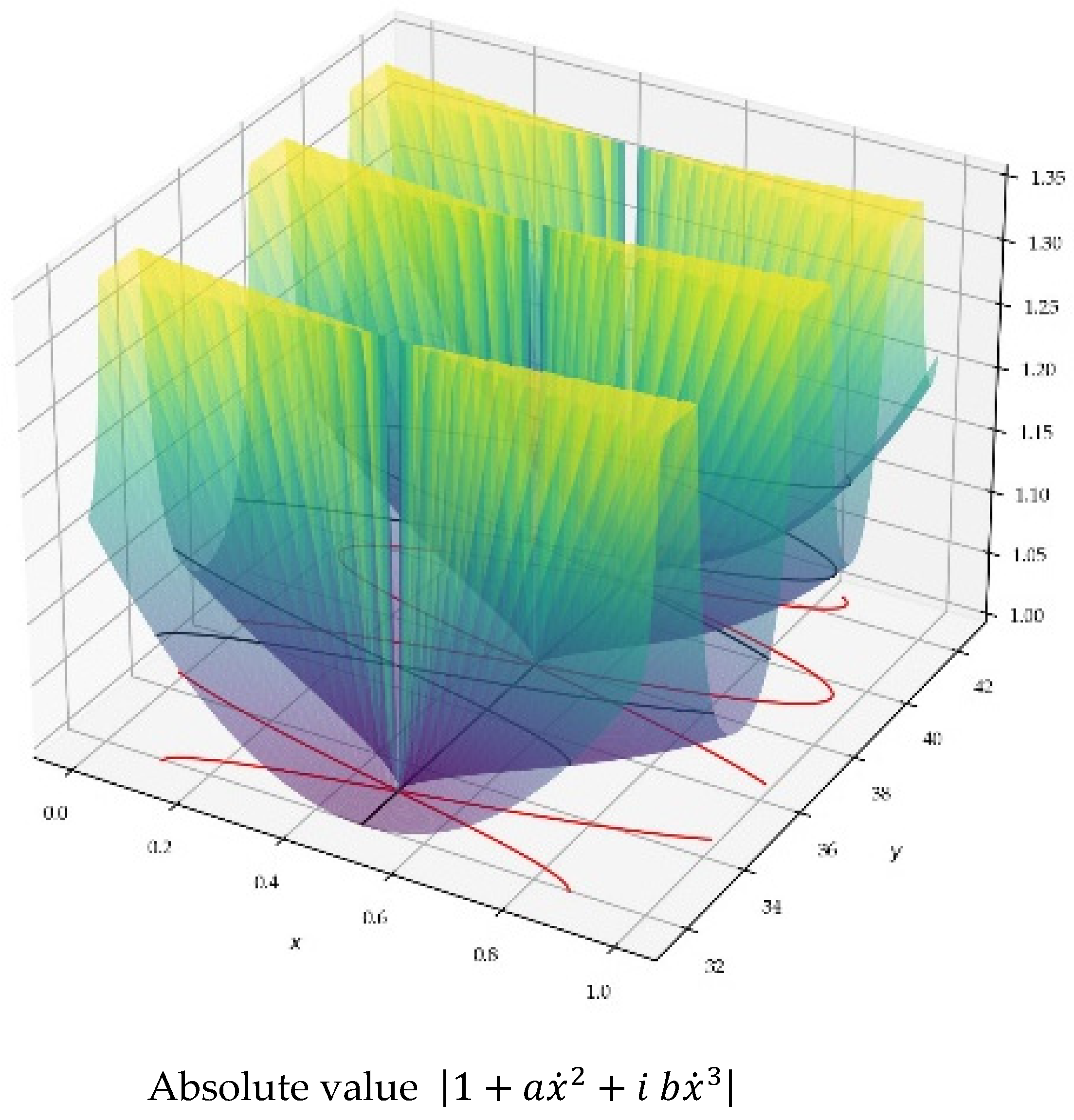
3.6. The Family of ${\mathrm{S}}_{\mathrm{m}}$ Functions

We further define, from $S$, the family of functions:

$$\forall m\in \mathbb{N}, \forall s\in ℂ\backslash \left\{poles, zeros\right\}:S_m\left(s\right)=-{\displaystyle \sum }_{Pôles}{\left(s-p_h\right)}^{-m}+{\displaystyle \sum }_{Zéros}{\left(s-z_n\right)}^{-m}$$

(12)

We thus obtain the following formulas for the calculation of the derivatives:

$$S_m^{\prime }\left(s\right)=-m{S}_{m+1}\left(s\right); S_1^{\left(m\right)}\left(s\right)={\left(-1\right)}^{m}m!S_{m+1}\left(s\right)$$

To calculate the successive derivatives of $S$, we therefore define the following series of functions, by separating the $P$ zeros of the CL and the possible $Q$ zeros of the CS:

$$S_m\left(s\right)=-({\left(s-0\right)}^{-m}+{\left(s-1\right)}^{-m})+{{\displaystyle \sum }}_{p=1}^P({\left(s-{𝓈}_p\right)}^{-m}+{(s-{\widehat{𝓈}}_p)}^{-m})+{{\displaystyle \sum }}_{q=1}^Q\left({\left(s-s_q\right)}^{-m}+{\left(s-{\widehat{s}}_q\right)}^{-m}\right)$$

For numerical calculations, it is important to consider the following case where only known zeros are considered, i.e., those of the CL. Numerical calculations are greatly simplified when we consider $𝓈$ on the CL and all the zeros $s_n=s_p$ taken in the calculation are on the CL:

$$\begin{gathered} S_m(𝓈)={\left(-1\right)}^m\left(-\frac{{\left(\text{½}+iy\right)}^m+{\left(-\text{½}+iy\right)}^m}{{\left(y^2+\text{¼}\right)}^m}+i^m{{\displaystyle \sum }}_{p=1}^{\infty }\frac{{\left(y-y_p\right)}^m+{\left(y+y_p\right)}^m}{{\left(y^2-y_p{}^2\right)}^m}\right) \\ {S}_1(𝓈)=-2iy\left(-\frac{1}{y^2+\text{¼}}+{{\displaystyle \sum }}_{p=1}^{\infty }\frac{1}{y^2-y_p{}^2}\right) \\ {S}_2(𝓈)=-2\left(-\frac{y^2-\text{¼}}{{\left(y^2+\text{¼}\right)}^2}+{{\displaystyle \sum }}_{p=1}^{\infty }\frac{y^2+y_p{}^2}{{\left(y^2-y_p{}^2\right)}^2}\right) \\ {S}_3(𝓈)=2iy\left(-\frac{y^2-\text{¾}}{{\left(y^2+\text{¼}\right)}^3}+{{\displaystyle \sum }}_{p=1}^{\infty }\frac{y^2+3y_p{}^2}{{\left(y^2-y_p{}^2\right)}^3}\right) \\ {S}_4(𝓈)=2\left(-\frac{y^4-\left(3/2\right)y^2+1/16}{{\left(y^2+\text{¼}\right)}^4}+{{\displaystyle \sum }}_{p=1}^{\infty }\frac{y^4+6y^2{y}_p{}^2+y_p{}^4}{{\left(y^2-y_p{}^2\right)}^4}\right) \\ {S}_5(𝓈)=-2iy\left(-\frac{y^4-\left(5/2\right)y^2+5/16}{{\left(y^2+\mathrm{¼}\right)}^5}+{{\displaystyle \sum }}_{p=1}^{\infty }\frac{y^4+10y^2{y}_p{}^2+5y_p{}^4}{{\left(y^2-y_p{}^2\right)}^5}\right) \end{gathered}$$

(13)

3.7. The Family of Composite $T_n$ Functions

We can express the successive derivatives $F^{\left(n\right)}$ of $F$ from the $S_m$ family. We further list the first nine terms of the derivative calculation:

$$\begin{gathered} F^{\prime }/F=T_1=S_1; F^{″}/F=T_2=S_1^2-S_2; F^{\left(3\right)}/F=T_3=S_1^3-3S_1{S}_2+2S_3 \\ {F}^{\left(4\right)}/F=T_4=S_1^4-6S_1^2{S}_2+3S_2^2+8S_1{S}_3-3!S_4 \\ {F}^{\left(5\right)}/F=T_5=S_1^5+5\left(-2S_1^3{S}_2+3S_1{S}_2^2+4S_1^2{S}_3-4S_2{S}_3-6S_1{S}_4\right)+4!S_5 \\ {F}^{\left(6\right)}/F=T_6=S_1^6+5\left(-3S_1^4{S}_2+9S_1^2{S}_2^2-3S_2^3+8S_1^3{S}_3-24S_1{S}_2{S}_3+8S_3^2-18S_1^2{S}_4+18S_2{S}_4\right)+6!S_1{S}_5/5-5!S_6 \\ \begin{array}{cc}\hfill F^{\left(7\right)}/F=T_7=S_1^7& \\ & +7(-3S_1^5{S}_2+15S_1^3{S}_2^2+10S_1^4{S}_3-60S_1^2{S}_2{S}_3+30S_2^2{S}_3-30S_1^3{S}_4-60S_3{S}_4-15S_1{S}_2^3\hfill \\ & +40S_1{S}_3^2+90S_1{S}_2{S}_4+72S_1^2{S}_5-72S_2{S}_5-5!S_1{S}_6)+6!S_7\hfill \\ \hfill F^{\left(8\right)}/F=T_8=S_1^8& \\ & +7(-4S_1^6{S}_2+30S_1^4{S}_2^2+16S_1^5{S}_3-160S_1^3{S}_2{S}_3-60S_1^4{S}_4+20S_1^2(-3S_2^3+8S_3^2+18S_2{S}_4)\hfill \\ & +48(4S_1^3{S}_5+S_1\left(5S_2^2{S}_3-10S_3{S}_4-12S_2{S}_5\right)+10S_2{S}_6-10S_1^2{S}_6))+8!S_1{S}_7/7-7!S_8\hfill \\ \hfill F^{\left(9\right)}/F=T_9=S_1^9& \\ & +9(-4S_1^7{S}_2\hfill \\ & +7(6S_1^5{S}_2^2-20S_1^3{S}_2^3+15S_1{S}_2^4+40\left(-S_1^4{S}_2+3S_1^2{S}_2^2-S_2^3\right)S_3\hfill \\ & +12\left(-S_1^5+10S_1^3{S}_2-15S_1{S}_2^2-20S_1^2{S}_3+20S_2{S}_3+15S_1{S}_4\right)S_4\hfill \\ & +48\left(S_1^4-6S_1^2{S}_2+3S_2^2+8S_1{S}_3-6S_4\right)S_5+160\left(-S_1^3+3S_1{S}_2-2S_3\right)S_6)\hfill \\ & +4\times 6!\left(S_1^2-S_2\right)S_7-7!S_1{S}_8)+8\times 7\left(3S_1^6{S}_3+60S_1^3{S}_3^2-120S_1{S}_2{S}_3^2+40S_3^3\right)+8!S_9\hfill \end{array} \end{gathered}$$

(14)

We can draw the cross-sections of the $F$ function, for different values of $y$, along $x$. We see the profile of the real and imaginary parts appear (Figure 6).

Figure 6. Drawings of several cross-sections of $F\left(s\right)$, when $s$ is not a zero: (a) real; (b) imaginary. On these different cross-sections at constant $y$ of the $F$ function, we observe the two symmetries which are characteristic of the function. The imaginary part is equal to zero for $x=½$, since they are cross-sections, not corresponding to non-trivial zeros. The colors are different depending on whether they are after a zero with an odd or an even index.

In Figure 7, we show the behavior of $F^{\left(n\right)}$ in 3D. The successive derivatives $F^{\left(n\right)}$ of $F$ appear as the product of the initial function $F$ and a factor $T_n$ which is a linear combination of various terms $S_m$, of order $n$, in powers of the rational fractions of this $S$ function. For the $F$ function, we have in $\mathcal{S}$ and on $ℒ:$

$$\forall s\in \mathcal{S}: F^{\left(n\right)}\left(s\right)=F\left(s\right)T_n\left(s\right); \forall 𝓈\in ℒ: F^{\left(n\right)}(𝓈)=F(𝓈)T_n(𝓈)$$

(15)

Figure 7. Plots of $F, F^{\prime }, F^{″}$: (a) real, (b) imaginary parts, and (c) modulus. The images of the different functions $F^{\left(n\right)}$ are similar, except that they exchange their real and imaginary aspects according to the parity of $n$.

In the following, pay attention to the $s=x+iy$ and $𝓈=\text{½}+iy$ which are to be distinguished.

We thus define a new family $T_n$ of composite functions, as a linear combination of rational fractions of singularity of order $\le m$, and this for all the poles and non-trivial zeros of the $S$ function. In $T_n\left(s\right)$, there are single $S$ terms, but there are also double and even triple terms. The possible multiplicity of zeros, here, is taken into account, by adding the rational fraction the same number of times.

$$T_n\left(s\right)={\displaystyle \sum }{\lambda }_p^{{\alpha }_p}{S}_p^{{\alpha }_p}+{\displaystyle \sum }{\lambda }_{p,q}^{{\alpha }_p,{\beta }_q}{S}_p^{{\alpha }_p}{S}_q^{{\beta }_q}+{\displaystyle \sum }{\lambda }_{p,q,r}^{{\alpha }_p,{\beta }_q,{\gamma }_r}{S}_p^{{\alpha }_p}{S}_q^{{\beta }_q}{S}_r^{{\gamma }_r}$$

More terms appear with increasing $n$. However, these terms are unimportant when using a Taylor series of low order, as these high order terms will disappear. The general term is:

$$T_n\left(s\right)={{\displaystyle \sum }}_{p=1,q=2,r=3}^n\left({\lambda }_{p,q,r}^{{\alpha }_p,{\beta }_q,{\gamma }_r}{S}_p^{{\alpha }_p}{S}_q^{{\beta }_q}{S}_r^{{\gamma }_r}\right);\lambda \in \mathbb{Z}; r>q>p; n=p{\alpha }_p+q{\beta }_q+r{\gamma }_r$$

(16)

We observe, for the first terms and the last term, a formula of the type:

$$\frac{F^{\left(n\right)}(𝓈)}{F(𝓈)}=T_n\left(s\right)={\left(S_1\right)}^n+{{\displaystyle \sum }}_{p=1}^n\left({\left(-1\right)}^{p-1}\left(p-1\right)!\left(\begin{array}{c}n\\ p\end{array}\right)S_1^{n-p}{S}_p\right)+\cdots +{\left(-1\right)}^{n+1}\left(n-1\right)!S_n$$

(17)

The $F$ function and the $\zeta$ function have challenging properties on the CL. For $x=½$, the real and imaginary parts of successive derivatives $F^{\left(n\right)}$ cancel each other out alternately. This property is also true numerically, even when considering any potential zeros out with the CL.

$$\forall n\in \mathbb{N},\forall 𝓈\in ℒ,\forall p 𝓈\ne {𝓈}_p :F^{\left(2n\right)}(𝓈)=a_{2n}+i\times 0\in ℝ; F^{\left(2n+1\right)}(𝓈)=0+i{b}_{2n+1}\in iℝ$$

(18)

These last observations will be useful for the following calculations.

3.8. Taylor’s Formula within the CS

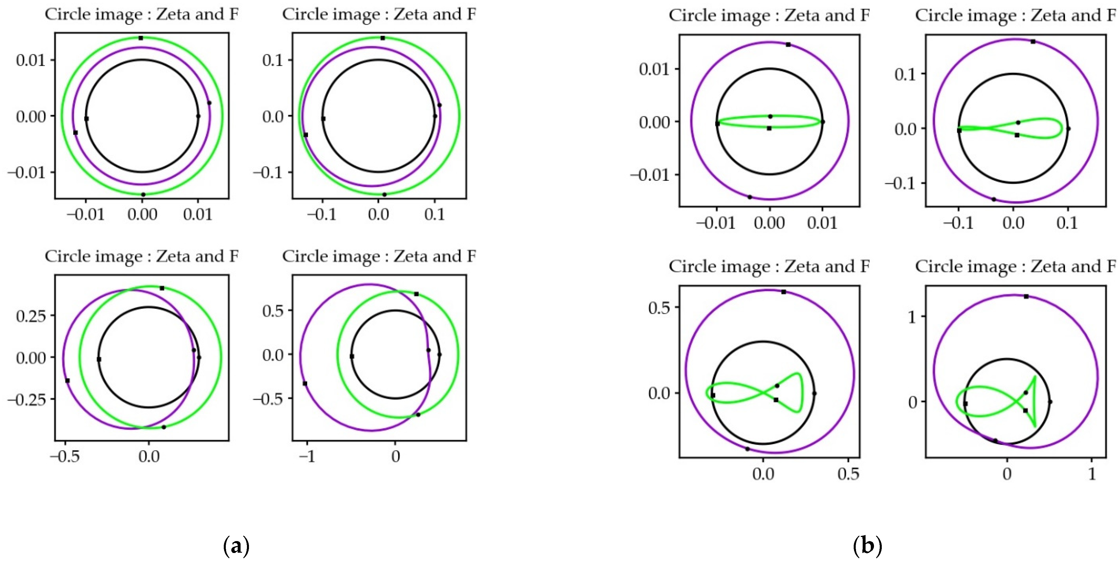
A holomorphic function is a conformal function: the image of a circle is a circle for small distances (Figure 8). The Taylor series of the $F$ function makes it possible to calculate the value $F\left(s\right)$ at a point $Z=s$ of the CS $\mathcal{S}$ in the vicinity of a point $H=𝓈$ of the CL $ℒ$, provided that $Z$ and $H$ are close ($\left|\right|Z-H\left|\right|<\epsilon \cong 1$). This is the direct numerical method.

Figure 8. Images of circles of different radii after transformations by $\zeta$ and $F$. Input image in black, $\zeta$ image in purple, $F$ image in green. Increasing the radius of the input image reduces the conformity of the projection, in both typical cases (a) and more extreme cases (b).

(a)

$H$ is not a non-trivial zero: $H\in ℒ\backslash \mathcal{Z}; F(𝓈)\ne 0$

The Taylor expansion of the $F$ function, of a point $Z=s$ in the CS from a point $H=𝓈$ on the CL is:

$$\begin{gathered} \forall s=x+i{y}_1\in \mathcal{S}, \forall 𝓈=\text{½}+i{y}_2\in ℒ:x\ll \left|y_1\right|; \left|y_1-y_2\right|<\epsilon <1; \Delta s=s-𝓈: \\ F\left(s\right)={{\displaystyle \sum }}_{n=0}^{\infty }\frac{{\left(s-𝓈\right)}^n}{n!}{F}^{\left(n\right)}(𝓈)={{\displaystyle \sum }}_{n=0}^{\infty }\frac{{\left(\Delta s\right)}^n}{n!}{F}^{\left(n\right)}(𝓈) \end{gathered}$$

(19)

$$\begin{gathered} \forall p 𝓈\ne {𝓈}_p: F\left(s\right)=F(𝓈)\left(1+{{\displaystyle \sum }}_{n=1}^{\infty }\frac{{\left(\Delta s\right)}^n}{n!}{T}_n(𝓈)\right)=F(𝓈)\left(A+iB\right) \\ \begin{array}{cc}\hfill F\left(s\right)=F(𝓈)(1 +& \Delta s S_1+\frac{{\left(\Delta s\right)}^2}{2!}\left(S_1^2-S_2\right)+\frac{{\left(\Delta s\right)}^3}{3!}\left(S_1^3-3S_1{S}_2+2!S_3\right)\hfill \\ & +\frac{{\left(\Delta s\right)}^4}{4!}\left(S_1^4-6S_1^2{S}_2+3S_2^2+8S_1{S}_3-3!S_4\right)\hfill \\ & +\frac{{\left(\Delta s\right)}^5}{5!}\left(S_1^5+5\left(-2S_1^3{S}_2+3S_1{S}_2^2+4S_1^2{S}_3-4S_2{S}_3-6S_1{S}_4\right)+4!S_5\right)+\cdots )\hfill \end{array} \end{gathered}$$

(20)

The Taylor expansion of the $F$ function, from a point on the CL is:

$$F\left(s\right)=F(𝓈)\left({{\displaystyle \sum }}_{k=0}^{\infty }\frac{{\left(s-𝓈\right)}^{2k}}{\left(2k\right)!}{T}_{2k}(𝓈)+{{\displaystyle \sum }}_{k=0}^{\infty }\frac{{\left(s-𝓈\right)}^{2k+1}}{\left(2k+1\right)!}{T}_{2k+1}(𝓈)\right);T_{2k}(𝓈)\in ℝ;T_{2k+1}(𝓈)\in iℝ$$

The $F$ function can be estimated numerically in the CS by taking an indirect route, according to a reasonable approximation, with only the first four or six terms, provided that a large number ($\mathsf{𝕡}>{10}^5$) of zeros is considered on the CL since the convergence of the poles and zeros function is slow. Moreover, the calculations are numerically unstable, as soon as $𝓈$ is quite close to a zero ${𝓈}_p$ of the CL, in which case a midpoint $y$ must be selected, for example: $𝓈=\text{½}+iy={𝓈}_p+\mathrm{¼}\left({𝓈}_{p+1}-{𝓈}_p\right)$ so as to avoid instability.

$$\begin{gathered} \forall s=x+i\left(y+dy\right)\in \mathcal{S} ; dy=\pm \epsilon ;\epsilon <1;\forall 𝓈=\text{½}+iy\in ℒ,𝓈\ncong {𝓈}_p,𝓈\ncong {𝓈}_{p+1};y_p<y<y_{p+1} : \\ F\left(s\right)\approx F(𝓈)\left(1+{{\displaystyle \sum }}_{n=1}^{\mathsf{𝕟}}\frac{{\left(s-𝓈\right)}^n}{n!}{T}_n(𝓈)\right);4\le \mathsf{𝕟}\le 6 \end{gathered}$$

In practice, the first four or six terms of the series will make it possible to estimate $F\left(s\right)$, with a good approximation, in the CS (Figure 9).

Figure 9. Exact $F$ (blue and red) and estimate of $F$ (lawn-green and brown) on a cross-section of CS from a point on the CL, using the Taylor series: (a) real part; (b) imaginary part. The approximate value corresponds well to the exact value. The approximation is less good when $\left|x-½\right|$ | increases.

If the points $Z$ and $H$ have the same y-coordinate, the expression is simplified:

$$\begin{gathered} \forall s=x+iy\in \mathcal{S}; 𝓈=\text{½}+iy\in ℒ: \\ F\left(s\right)=\frac{\Gamma \left(s/2\right)}{{\pi }^{s/2}}\zeta \left(s\right)=F(𝓈)T\left(s,𝓈\right)=\frac{\Gamma \left(𝓈/2\right)}{{\pi }^{𝓈/2}}\zeta (𝓈)\left(1+i{b}_1\dot{x}+\frac{a_2}{2!}{\dot{x}}^2+i\frac{b_3}{3!}{\dot{x}}^3+\frac{a_4}{4!}{\dot{x}}^4+\cdots \right) \\ \forall k\in \mathbb{N}:\left|\right|\frac{{\dot{x}}^{2k}}{\left(2k\right)!}{T}_{2k}\left|\right|>\left|\right|\frac{{\dot{x}}^{2k+2}}{\left(2k+2\right)!}{T}_{2k+2}\left|\right|;\left|\right|\frac{{\dot{x}}^{2k+1}}{\left(2k+1\right)!}{T}_{2k+1}\left|\right|>\left|\right|\frac{{\dot{x}}^{2k+3}}{\left(2k+3\right)!}{T}_{2k+3}\left|\right| \\ \forall m\in \mathbb{N}:\left|\right|S_{2m}\left|\right|>\left|\right|S_{2m+2}\left|\right|;\left|\right|S_{2m+1}\left|\right|>\left|\right|S_{2m+3}\left|\right| \end{gathered}$$

The $T_n$ are calculated from:

$$S(𝓈)\approx -2iy\left(-\frac{1}{y^2+\mathrm{¼}}+{{\displaystyle \sum }}_{p=1}^{\mathsf{𝕡}}\frac{1}{y^2-y_p^2}\right);\mathsf{𝕡}>{10}^5$$

We know how to exactly calculate the value $F\left(x+iy\right)$ thanks to the theoretical formula using the special functions and, in our study, we calculate $F\left(x+iy\right)$ in a second way, using the Taylor expansion under the form of the product of $F\left(½+iy\right)$ and a polynomial. The knowledge of the theoretical formula makes it possible to validate the efficacy of the approximate formulas. The error, made with Taylor’s formula, taking into account only the first $\mathsf{𝕟}$ terms, is known:

$$e_{\mathsf{𝕟}}\left(x,y\right)=\frac{\Gamma \left(\left(x+iy\right)/2\right)}{{\pi }^{\left(x+iy\right)/2}}\zeta \left(x+iy\right)-{{\displaystyle \sum }}_{n=0}^{\mathsf{𝕟}}{F}^{\left(n\right)}\left(½+iy\right)\frac{{\left(x-½\right)}^n}{n!}$$

$$e_{\mathsf{𝕟}}\left(x,y\right)={{\displaystyle \sum }}_{n=\mathsf{𝕟}+1}^{\infty }{F}^{\left(n\right)}\left(½+iy\right)\frac{{\left(x-½\right)}^n}{n!}\cong F^{\left(\mathsf{𝕟}+1\right)}\left(½+iy\right)\frac{{\left(x-½\right)}^{\mathsf{𝕟}+1}}{\left(\mathsf{𝕟}+1\right)!}$$

$$e_{\mathsf{𝕟}}\left(x,y\right)=F\left(½+iy\right)\times T_{\mathsf{𝕟}+1}\left(½+iy\right)\frac{{\left(x-½\right)}^{\mathsf{𝕟}+1}}{\left(\mathsf{𝕟}+1\right)!}$$

The factor $T_{\mathsf{𝕟}+1}\left(½+iy\right)$ varies in $y^{-\left(\mathsf{𝕟}+1\right)},$ as a linear combination of functions $S$ of order $\mathsf{𝕟}+1$. The term $S=F^{\prime }/F$ is also known thanks to the theoretical formula of $F^{\prime }$ and $F$. We can therefore calculate the error that we make by taking into account only a finite number $\mathsf{𝕡}$ of zeros. We realize, after analysis, that it is necessary to take a large number of zeros if we want to correctly approach the value $S$. The slow convergence of the expressions $S_m\left(y\right)$ in the Formulas (13) comes from the sum of rational functions ${\left(y-y_p\right)}^{-m},$ as can be seen in Figure 5.

$$e_{\mathsf{𝕟}}\left(x,y\right)\cong \frac{F\left(½+iy\right)}{\left(\mathsf{𝕟}+1\right)!}\mathcal{O}\left({\left(\frac{x-½}{y}\right)}^{\mathsf{𝕟}+1}\right)$$

The value of $T_{\mathsf{𝕟}+1}$ in fact makes it possible to define the stopping condition for the algorithm calculating $F\left(s\right)$, where the value of $y$ is preponderant.

Indeed, the reasoning appeals to a series expansion, which numerically gives good results (Figure 10) since the CS is narrow, and the maximum difference between a point $s$ and the closest point $𝓈$ is at most $½$. Table 4 illustrates the accuracy of the series expansion for different ordinates between $s$ and $𝓈$.

Figure 10. (a) Direct and indirect estimates of $F$ in comparison with the true value of $F$ : we observe that $\Re \left(F\right)$ and $\Im \left(F\right)$ never intersect at zero together. We observe the ‘fairy chimneys’, which are artefacts of the numerical calculation. (b) $S_1$ (blue), $S_2$ (red), $S_3$ (green), $S_4$ (cyan) curves along $y$ for $x=0.05$ : $S_2$ and $S_4$ do not cross the zero ordinate. $S_2$ is always negative.

Table 4. General case not close to a zero: $F$ estimation in the CS from the CL (same $y$) via both methods with $F^{\left(n\right)}$ and $T_n$. This table shows the good accuracy of the $F$ estimation with eight terms using the indirect way, with various $y:100, {10}^3, {10}^4$.

$\mathit{s}=\mathit{x}+\mathit{i}\mathit{y}$	True F(s) Value	F * Direct Way (9 Derivatives)	F * Indirect Way (8 Terms)
$1/10+i100$	$1.466 977 65-i 0.430 829 31$	$1.466 977 99-i 0.430 829 35$	$1.467 002-i 0.430 744$
$1/10+i1 000$	$0.518 493+i 0.496 115 9$	$0.518 483 +i 0.496 118 6$	$0.518 20+i 0.496 41$
$1/10+i10 000$	$0.348 988+i 0.365 27$	$0.348 960+i 0.365 31$	$0.346 8+i 0.367 3$

Now we can enhance the calculation. There are several ways to group terms according to the characteristics of $T_n\left(s\right)$:

$$e^{\Delta s S_1}=1+\Delta s S_1+\frac{{\left(\Delta s S_1\right)}^2}{2!}+\frac{{\left(\Delta s S_1\right)}^3}{3!}+\dots$$

$$F\left(s\right)=F(𝓈)\left(e^{{\Delta s S}_1}-\frac{{\left(\Delta s\right)}^2}{2}{S}_2{e}^{{\Delta s S}_1}+\frac{{\left(\Delta s\right)}^3}{3}{S}_3{e}^{{\Delta s S}_1}-\frac{{\left(\Delta s\right)}^4}{4}\left(S_4-{\text{½}S}_2^2\right)e^{{\Delta s S}_1}+\frac{{\left(\Delta s\right)}^5}{5}\left(S_5-⅙5S_2{S}_3\right)e^{{\Delta s S}_1}+\cdots \right)$$

This way makes it possible to reveal and factor the term $e^{\Delta s S_1}$, which is fundamental for the following reasoning.

$$\begin{gathered} F\left(s\right)=F(𝓈)e^{\Delta s{S}_1}(1-{{\displaystyle \sum }}_{k=2}^{\infty }\frac{{\left(-\Delta s\right)}^k}{k}{S}_k+\frac{{\left(\Delta s\right)}^4}{8}{S}_2^2-\frac{{\left(\Delta s\right)}^5}{6}{S}_2{S}_3+\frac{{\left(\Delta s\right)}^6}{8}{S}_2{S}_4-\frac{{\left(\Delta s\right)}^6}{48}{S}_2^3+\frac{{\left(\Delta s\right)}^6}{18}{S}_3^2 \\ +\frac{{\left(\Delta s\right)}^7}{24}{S}_2^2{S}_3-\frac{{\left(\Delta s\right)}^7}{12}{S}_3{S}_4-\frac{{\left(\Delta s\right)}^7}{10}{S}_2{S}_5+\frac{{\left(\Delta s\right)}^8}{12}{S}_2{S}_{6+}\dots ) \end{gathered}$$

The full form is as follows, with the general term:

$$F\left(s\right)=F(𝓈)e^{\Delta s{S}_1}\left(1+{{\displaystyle \sum }}_{k,l,m,\alpha ,\beta ,\gamma }^{\infty }{\lambda }_{k,l,m,\alpha ,\beta ,\gamma }{\left(\Delta s\right)}^{\alpha k+\beta l+\gamma m}{S}_k^{\alpha }{S}_l^{\beta }{S}_m^{\gamma }\right);m>l>k>1;\alpha ,\beta ,\gamma \ge 0$$

If $\Delta y=0$, i.e., when $H$ has the same ordinate as $Z$, things get simpler:

$$\begin{gathered} \Delta s=\Delta x+i \Delta y \\ \Delta y=0 \Rightarrow \Delta s S_1=\dot{x }{S}_1=i\theta \\ \begin{array}{cc}\hfill F\left(s\right)=F(𝓈)e^{\dot{x} S_1}& (1-{\displaystyle \sum }_{p=2}^{\infty }\frac{{\left(-\dot{x}\right)}^p}{p}{S}_p+{\displaystyle \sum }_{p>1,q>p}^{\infty }\frac{{\left(-\dot{x}\right)}^{p+q}}{pq}{S}_p{S}_q\pm {\displaystyle \sum }_{p,r>1,q>p}^{\infty }\frac{{\left(-\dot{x}\right)}^{pr+q}}{p^{r}qr!}{S}_p^r{S}_q\hfill \\ & \pm {{\displaystyle \sum }}_{p,r>1 }^{\infty }\frac{{\left(-\dot{x}\right)}^{pr}}{p^{r}r!}{S}_p^r+\cdots )\hfill \end{array} \\ F\left(s\right)=F(𝓈)e^{i\theta }(1+\frac{{\dot{x}}^2}{2}\left(-S_2\right)+\frac{{\dot{x}}^3}{3}{S}_3-\frac{{\dot{x}}^4}{4}\left(S_4-\text{½}{S}_2^2\right)+\frac{{\dot{x}}^5}{5}\left(S_5-⅙5S_2{S}_3\right)-\frac{{\dot{x}}^6}{6}\left(S_6+\mathrm{⅛}{S}_2^3-\mathrm{⅓}{S}_3^2-\text{¾}{S}_2{S}_4\right) \\ +\frac{{\dot{x}}^7}{7}\left(S_7+\text{½}7\left(S_2^2{S}_3/12-⅙S_3{S}_4-⅕S_2{S}_5\right)\right)+\cdots )=F(𝓈)e^{i\theta }\left(1+a{\dot{x}}^2+ib{\dot{x}}^3+\cdots \right) \end{gathered}$$

(21)

$F$ vanishes for the real and imaginary parts when $\theta =½\pi +k\pi$ and $\theta =k\pi$, which gives the frequency of the alternating zeros of $F$ in the CS. With this formula, we thus obtain the coordinates $\left(x,y\right)$ for which the two components of the value $F\left(s\right)$ cancel each other out alternately and periodically. $\theta$ depends on $\left(x,y\right)$ but the influence of $x$ is small. It is for this reason that on the graphs in Figure 7, zero iso-contours appear as lines perpendicular to the y-axis (while they can also be approximated as flat polynomials). For $x\ne ½$, the two components of $F\left(s\right)$ are periodically zero, at a half rhythm of those of $\zeta$, in the interval $\left[y_p, y_{p+1}\right]$ and this on the anamorphic scale of $\tilde{y}$.

We conclude that we have found several expressions of $F$:

$$\begin{gathered} \forall s\in \mathcal{S}; \zeta (𝓈)\ne 0;F(𝓈)=\Gamma \left(𝓈/2\right){\pi }^{-𝓈/2}\zeta (𝓈) \\ F\left(s\right)=F(𝓈)\left(A+iB\right)=F(𝓈)e^{i\theta }\left(1+{a\dot{x}}^2+{i b\dot{x}}^3+\dots \right) \\ {\dot{x}S}_1(𝓈)=i\theta ;p\left(s,𝓈\right)={{\displaystyle \sum }}_{n=1}^{\infty }{a}_{2n}{\dot{x}}^{2n}+i{{\displaystyle \sum }}_{n=1}^{\infty }{b}_{2n+1}{\dot{x}}^{2n+1};\theta ,{ a}_{2n},{ b}_{2n+1}\in ℝ \\ \begin{array}{cc}\hfill p\left(s,𝓈\right)=-\frac{{\dot{x}}^2}{2}{S}_2& +\frac{{\dot{x}}^3}{3}{S}_3-\frac{{\dot{x}}^4}{4}\left(S_4-{\text{½}S}_2^2\right)+\frac{{\dot{x}}^5}{5}\left(S_5-⅙5S_2{S}_3\right)-\frac{{\dot{x}}^6}{6}\left(S_6+\mathrm{⅛}{S}_2^3-\mathrm{⅓}{S}_3^2-{\text{¾}S}_2{S}_4\right)\hfill \\ & +\frac{{\dot{x}}^7}{7}\left(S_7+\text{½}7\left(S_2^2{S}_3/12-⅙{ S}_3{S}_4-⅕S_2{S}_5\right)\right)+\cdots \hfill \end{array} \\ F\left(s\right)=F(𝓈)e^{i\theta }\left(1+p\left(s,𝓈\right)\right) \end{gathered}$$

(22)

(b)

$H$ is a non-trivial zero: $H\in \mathcal{Z};\zeta \left(H\right)=0\Rightarrow F\left(H\right)=0$

It remains to deal with the case where there exists a zero of the $\zeta$ function on the CL at $y_p$. When $s$ is zero, Hadamard’s product formula as a logarithm does not apply, so we have to consider $F\left(s\right)$ and its derivatives under the direct formula. In this case, we will therefore seek a relationship between the Hadamard product formula and the associated formulas, which we will relate to the direct calculation. The formulas are a little different $F^{″}\left(s\right)/F^{\prime }\left(s\right)=S_1\left(s\right)={\zeta }^{\prime }\left(s\right)$, but this will help us stick to the general results. As the function $F$ is holomorphic, the ‘fairy chimneys’ that appear numerically are in fact computational artifacts, which do not represent the reality of the $F$ function.

When $\zeta \left(½+iy\right)=0$, a similar calculation gives the following result:

$$\begin{gathered} \forall s\in \mathcal{S};\forall 𝓈=\text{½}+iy: \zeta (𝓈)=0 \Rightarrow F\left(s\right)=G(𝓈)\left(e^{i\theta }\left(1+p\left(s,𝓈\right)\right)-1\right) \\ G(𝓈)=\Gamma \left(𝓈/2\right){\pi }^{-𝓈/2};{ S}_1={\zeta }^{\prime }(𝓈);{\dot{x}S}_1(𝓈)=i\theta \\ p\left(s,𝓈\right)={{\displaystyle \sum }}_{n=1}^{\infty }{a}_{2n}{\dot{x}}^{2n}+i{{\displaystyle \sum }}_{n=1}^{\infty }{b}_{2n+1}{\dot{x}}^{2n+1};\theta ,{ a}_{2n},{ b}_{2n+1}\in ℝ \\ p\left(s,𝓈\right)=-\frac{{\dot{x}}^2}{2}{S}_2+\frac{{\dot{x}}^3}{3}{S}_3-\frac{{\dot{x}}^4}{4}\left(S_4-\text{½}{S}_2^2\right)+\frac{{\dot{x}}^5}{5}\left(S_5-⅙5S_2{S}_3\right)-\frac{{\dot{x}}^6}{6}\left(S_6+\mathrm{⅛}{S}_2^3-\mathrm{⅓}{S}_3^2-\text{¾}{S}_2{S}_4\right) \\ +\frac{{\dot{x}}^7}{7}\left(S_7+\text{½}7\left(S_2^2{S}_3/12-⅙ S_3{S}_4-⅕S_2{S}_5\right)\right)+\cdots \end{gathered}$$

(23)

We can draw the cross-sections of the $F$ function, for different values of $y_p$, along $x$. We see the profile of the real and imaginary parts appear (Figure 11).

Figure 11. Drawings of several $F$ cross-sections, when $s_p$ is a zero. On these different cross-sections at constant $y$ of the $F$ function, we observe the two symmetries which are characteristic of the function. The two real and imaginary parts are equal to zero for $x=½$, since they are cross-sections corresponding to non-trivial zeros. The colors are different depending on whether they are zeros with an odd or even index.

3.9. The Numerical RH Debate

When we estimate the value $F\left(s\right)$ of $Z$ in the CS, from the information of the point $H$ on the CL at coordinate $𝓈$, a contradiction arises when we assume that the point $Z$ in the CS is itself a zero.

(a)

$H$ is not a non-trivial zero: $H\in ℒ\backslash \mathcal{Z}; F(𝓈)\ne 0$

If $H \left(\forall p:𝓈\ne {𝓈}_p\Rightarrow F(𝓈)\ne 0 \right)$ is not a non-trivial zero of the CL $ℒ$, then $Z$ can be a zero $s=s_q$ of the CS $\mathcal{S}$, provided that $A$ and $B$ are zero at the same time:

$$\forall 𝓈 \forall p 𝓈\ne {𝓈}_p\Rightarrow \zeta (𝓈)\ne 0\Rightarrow F(𝓈)\ne 0;s\in \mathcal{S}\Rightarrow \dot{x}\ne 0;F\left(s\right)=F\left(s_q\right)=0\Rightarrow A=B=0$$

(24)

This is impossible: the dead end appears in the expression $e^{i\theta }\left(1+a{\dot{x}}^2+i b{\dot{x}}^3\right)$.

$$A+iB=e^{i\theta }\left(1+a{\dot{x}}^2+i b{\dot{x}}^3\right);e^{i\theta }\ne 0 \wedge 1+a{\dot{x}}^2+i b{\dot{x}}^3\ne 0.$$

Indeed, the real and imaginary parts of the exponential $e^{i\theta }$ cancel each other out periodically and alternately. On Figure 12, we also show that the polynomial $1+{\dot{x}}^{2}a+i b{\dot{x}}^3$ does not cancel, when in the CS.

$$\sqrt{{\left(1+a{\dot{x}}^2\right)}^2+{\left(b{\dot{x}}^3\right)}^2}>1$$

$$\forall 𝓈 \forall p 𝓈\ne {𝓈}_p\Rightarrow \zeta (𝓈)=\zeta \left(\text{½}+iy\right)\ne 0\Rightarrow F(𝓈)\ne 0;s=x+iy\in \mathcal{S}\Rightarrow \dot{x}\ne 0;\left|F\left(s\right)\right|>\left|F(𝓈)\right|>0$$

(25)

Figure 12. $1+a{\dot{x}}^2+i b{\dot{x}}^3$; 3D plot of the modulus of the polynomial $1+a{\dot{x}}^2+i b{\dot{x}}^3$. On this 3D image, we observe that the modulus of the polynomial expression vanishes only on the CL, in accordance with the RH.

Moreover, if the RH is false, it means that there exists at least one value for which $F$ (therefore$\zeta$) vanishes.

$$\exists q\in \mathbb{N},\exists s_q=x_q+i{y}_q\in \mathcal{S}\backslash ℒ; x_q\ne ½ :\zeta \left(s_q\right)=\zeta \left({\widehat{s}}_q\right)=0\iff F\left(s_q\right)=F\left({\widehat{s}}_q\right)=0$$

$$F\left(s_q\right)=F(𝓈)\left(A+iB\right)\Rightarrow \left(\left(F(𝓈)=0\right)\vee \left(A=0 \wedge B=0\right)\right)$$

We are therefore going to be directly aligned on the same $y_q$ with this point to calculate $F\left(s_q\right)$ from $F\left({𝓈}_q\right)$. The main formula remains:

$$\forall s\in \mathcal{S};\forall 𝓈\ne {𝓈}_p\Rightarrow F(𝓈)\ne 0 : F\left(s\right)=F(𝓈)\left(1+{{\displaystyle \sum }}_{n=1}^{\infty }{a}_n{\frac{\dot{x}}{n!}}^n\right); a_n\in ℂ$$

$a_n$ is a linear combination of terms, at least one element of which includes the term $\frac{1}{s-s_q}$. When $s$ is precisely equal to $s_q$, these terms are undefined, which is in contradiction with the fact that $F\left(s_q\right)=0$. The contradiction is glaring here:

$$F\left(s_q\right)=0=F\left({𝓈}_q\right)\left(C+{{\displaystyle \sum }}_{m=1}^{\infty }{\mu }_m\left(\frac{1}{s_q-s_q}\right)\right)=\infty ;F\left({𝓈}_q\right)\ne 0; {\mu }_m\ne 0 ;C,{\mu }_m\in ℂ$$

$$\forall n>0:T_n=U_n+V_n;\left|U_n\right|<\infty ;\exists j\in \mathbb{N}:{\mu }_j\ne 0: V_n={{\displaystyle \sum }}_{j=1}^n{\mu }_j\frac{1}{{\left(s_q-s_q\right)}^j};\left|V_n\right|=\infty$$

$$\forall n>0: T_n=\infty \Rightarrow A=B=\infty$$

This is particularly the case ($j=1$) for the first term $T_1$, if $s=s_q$:

$$T_1=S\left(s_q\right)=-\left(\frac{1}{s_q}+\frac{1}{s_q-1}\right)+{{\displaystyle \sum }}_{n=1,n\ne q}^{\infty }\left(\frac{1}{s_q-s_n}\right)+\frac{1}{s_q-s_q}=U_1+\frac{1}{s_q-s_q}=\infty$$

This contradiction establishes that zeros do not exist in the CS $\mathcal{S}\backslash ℒ$. Hence, $Q=0$.

(b)

$H$ is a non-trivial zero: $H\in \mathcal{Z};\zeta \left(H\right)=0\Rightarrow F\left(H\right)=0$

However, it remains to deal with the particular teratological case where $s=s_q\in \mathcal{S}$ would be in line with a zero $𝓈={𝓈}_p\in ℒ$ on the CL. In Figure 13, we observe, for the first 100 zeros that $\left|F\left(s\right)\right|>\left|F(𝓈)\right|>0$ and $\left|e^{i\theta }\left(1+a{\dot{x}}^2+i b{\dot{x}}^3\right)-1\right|>0$. The same reasoning as a) applies, except that Taylor’s formula is:

$$\begin{gathered} \forall 𝓈 \forall p 𝓈={𝓈}_p=\text{½}+{iy}_p;s_q=x+{iy}_q\in \mathcal{S}\backslash ℒ;y_q=y_p;\dot{x}=s_q-{𝓈}_p=x-\text{½}\ne 0;\zeta \left({𝓈}_p\right)=0\Rightarrow F\left({𝓈}_p\right)=0 \\ F\left(s_q\right)=G\left({𝓈}_p\right)\left(e^{i\theta }\left(1+{a\dot{x}}^2+{i b\dot{x}}^3\right)-1\right);G\left({𝓈}_p\right)=\Gamma \left(\text{½}{𝓈}_p\right)/{\pi }^{\text{½}{𝓈}_p}\ne 0;e^{i\theta }\left(1+{a\dot{x}}^2+i {b\dot{x}}^3\right)\ne 1 \\ \left|F\left(s\right)\right|>\left|F(𝓈)\right|>0 \end{gathered}$$

(26)

Figure 13. 3D plot ($x, index of \zeta zeros)$: On these 3 images, we observe that the modulus of the estimated function $F$, of the true $F$ function and of the exponential and polynomial expression cancel each other out only on the CL, in accordance with the RH, and this for cross-sections with non-trivial zeros. (a) estimated $\left|F\left(\mathrm{s}\right)\right|$; (b) true $\left|F\left(\mathrm{s}\right)\right|$; (c) $\left|e^{i\theta }\left(1+a{\dot{x}}^2+i b{\dot{x}}^3\right)-1\right|$.

4. Discussion

4.1. The $F$ Function as an Integral

If we analyze the RH through the prism of the $ℱℰ$ of the $\zeta$ function in the form of the integral of Jacobi’s theta [29] and Euler’s gamma functions, the function to be integrated has enormous oscillations in both its periods and its amplitudes (Figure 14). By concealing and dissolving the $\zeta$ function in an integral, B. Riemann established his $ℱℰ$.

$$F\left(s\right)=\frac{\Gamma \left(s/2\right)}{{\pi }^{s/2}}\zeta \left(s\right)={{\displaystyle \int }}_0^{\infty }\frac{\vartheta \left(0;iu\right)-1}{2}{u}^{s/2}\frac{du}{u}$$

$$\widehat{s}=1-s; {\varpi }_n=n^2\pi ; F\left(s\right)={{\displaystyle \int }}_0^{\infty }{{\displaystyle \sum }}_{n=1}^{\infty }{e}^{-{\varpi }_{n}u}{u}^{s/2}\frac{du}{u}={{\displaystyle \int }}_1^{\infty }{{\displaystyle \sum }}_{n=1}^{\infty }{e}^{-{\varpi }_{n}u}\left(u^{s/2}+u^{\widehat{s}/2}\right)\frac{du}{u}-\left(\frac{1}{s}+\frac{1}{\widehat{s}}\right)=F\left(\widehat{s}\right)$$

Figure 14. (a,b) Instability of the calculation of the integral due to strong variations in the function of $u$ (after removing the overall influence of the exponential part) to be integrated, for the first $n$ terms. The numerical calculation of the integral requires a very large number of samples of the value of the integrand function (around ten million between ${10}^{-2}$ and $1$).

After the sum and integral signs are inverted, the integral resolves as integral exponentials, or incomplete gamma functions.

$$F\left(s\right)={{\displaystyle \sum }}_{n=1}^{\infty }{{\displaystyle \int }}_0^{\infty }{e}^{-{\varpi }_{n}u}{u}^{s/2}\frac{du}{u}={{\displaystyle \sum }}_{n=1}^{\infty }{{\displaystyle \int }}_1^{\infty }{e}^{-{\varpi }_{n}u}\left(u^{s/2}+u^{\widehat{s}/2}\right)\frac{du}{u}-\left(\frac{1}{s}+\frac{1}{\widehat{s}}\right)$$

$$F\left(s\right)+\left(\frac{1}{s}+\frac{1}{\widehat{s}}\right)={{\displaystyle \sum }}_{n=1}^{\infty }\left(\frac{\gamma \left(s/2, {\varpi }_n\right)}{ {\varpi }_n{}^{s/2}}+\frac{\gamma \left(\widehat{s}/2, {\varpi }_n \right)}{ {\varpi }_n{}^{\widehat{s}/2}}\right); \gamma \left(s,a \right)={{\displaystyle \int }}_0^a{e}^{-u}{u}^s\frac{du}{u}$$

The infinite sum is of the order of magnitude of the term $\left(s^{-1}+{\widehat{s}}^{-1}\right)$, and its terms decrease very quickly. $\left(s^{-1}+{\widehat{s}}^{-1}\right)$ is almost equal to the first term, which explains the extremely low value of $F$ as $y$ increases. The $F$ integral therefore appears in the form of a sum of incomplete gamma functions, themselves developed in series, using the Pochhammer’s symbol.

$$F\left(s\right)+\left(\frac{1}{s}+\frac{1}{\widehat{s}}\right)={{\displaystyle \sum }}_{n=1}^{\infty }{e}^{-{\varpi }_n}\left({{\displaystyle \sum }}_{k=0}^{\infty } {\varpi }_n{}^k\left(\frac{1}{{\left(s/2\right)}_{k+1}}+\frac{1}{{\left(\widehat{s}/2\right)}_{k+1}}\right)\right)$$

Numerical evaluation of incomplete gamma functions $\gamma \left(s,a\right)$ has been the subject of research for many years [30,31,32]. Little progress has been made with a complex parameter $s$: hence, the value $\gamma \left(s/2,{\varpi }_n\right)$ is difficult to evaluate numerically in the CS. From the second term onwards ($n\ge 2$), terms are very close in absolute value, and form an alternating series with positive and or negative (real and imaginary) components. The numerical calculations of $F$ are therefore delicate and unstable as soon as $y>30$.

Thus, in the CS, following numerical calculations using incomplete gamma functions or Kummer’s confluent hypergeometric functions [33], the graphical and numerical behavior of the integral appears as a mille-feuille (layering) of Pochhammer surfaces $F_k\left(s\right)$. These surfaces have simple symmetry properties, at the origin of the $ℱℰ$ and at the source of the RH.

$$\frac{1}{{\left(s/2\right)}_{k+1}}={{\displaystyle \prod }}_{p=0}^k\frac{1}{s/2+p}=\frac{\Gamma \left(s/2\right)}{\Gamma \left(s/2+k+1\right)}={{\displaystyle \sum }}_{p=0}^k\frac{{\left(-1\right)}^p}{p!\left(k-p\right)!}\frac{1}{\left(s/2+p\right)}$$

$$F\left(s\right)+\left(\frac{1}{s}+\frac{1}{\widehat{s}}\right)={{\displaystyle \sum }}_{n=1}^{\infty }{e}^{-{\varpi }_n}\left({{\displaystyle \sum }}_{k=0}^{\infty } {\varpi }_n{}^k\left({{\displaystyle \sum }}_{p=0}^k\frac{{\left(-1\right)}^p}{p!\left(k-p\right)!}\left(\frac{1}{s/2+p}+\frac{1}{\widehat{s}/2+p}\right)\right)\right)$$

$$F\left(s\right)={\displaystyle \sum }{\lambda }_k\left(\frac{1}{{\left(s/2\right)}_{k+1}}+\frac{1}{{\left(\widehat{s}/2\right)}_{k+1}}\right)={\displaystyle \sum }{\mu }_k{F}_k\left(s\right); F_k\left(s\right)={\left(s+2k\right)}^{-1}+{\left(\widehat{s}+2k\right)}^{-1}$$

The $F$ function is therefore a layering of Pochhammer surfaces (Figure 15), where the RH emerges graphically. Indeed, we observe symmetries in both its real and imaginary components. In the case of the real part, the symmetry is a plane, and for the imaginary part, there is a line of symmetry at $x=½$. It is clear the CL is fertile, as its imaginary part is zero on this entire line. Non-trivial zeros therefore occur when the real part is zero, which happens periodically.

Figure 15. Pochhammer surfaces: the resemblance of the surfaces with those of Figure 3 and Figure 7 is striking. The $F$ function is generated by a sum of Pochhammer surfaces.

The nullity of the real part is periodically present, all along the CS on very flattened polynomial curves, appearing as almost straight lines perpendicular to the CL. The imaginary part is similarly zero on a different set of polynomial curves, in the CS, outside the CL. The RH would therefore be false if the zero iso-values of the two surfaces crossed in the CS, outside of the CL. In fact, the phenomenon does not occur, which we can glimpse graphically and understand numerically, by investigating the power series.

4.2. The Comparison with the $\zeta$ Version in Finite Fields

Analogies exist between the field of numbers and the fields of functions over a finite field, i.e., between the field $\mathbb{Q}$ and the field ${\mathbb{F}}_p\left(X\right)$ (and their finite extensions). Intuitively and schematically, the correspondence rests on the points where a curve meets the crossings of a grid of a sheet of checkered paper, drawn on the scale of algebraic integers. The $\zeta$ function zeros are the zeros of an irreducible polynomial $P$ (e.g., $X^3+X^2+X+1=0$) represented by a smooth planar curve $\mathcal{C}\left(x,y\right)$, on which we establish congruences in a space ${\mathbb{F}}_q$ from a prime number to a certain power $q=p^f,\left(\mathrm{e}.\mathrm{g}., {\mathbb{F}}_{49};49=7^2\right)$. The $\zeta$ function, associated with the curve, satisfies the properties of the $ℱℰ$ and the RH [34,35].

The $\zeta$ function is:

$$Z\left(\mathcal{C}/{\mathbb{F}}_q,t\right)=\frac{{{\displaystyle \prod }}_{j=1}^g\left(1-{\omega }_{j}t\right)\left(1-{\widehat{\omega }}_{j}t\right)}{\left(1-p_{1}t\right)\left(1-{\widehat{p}}_{1}t\right)}=\frac{{{\displaystyle \prod }}_{j=1}^g\left(1-{\omega }_{j}t\right)\left(1-{\overline{\omega }}_{j}t\right)}{\left(1-p_{1}t\right)\left(1-{\widehat{p}}_{1}t\right)}$$

$$\forall j:{\widehat{\omega }}_j={\overline{\omega }}_j;\left|{\omega }_j\right|=\sqrt{q}; {\omega }_j{\overline{\omega }}_j=q; p_1=1$$

The $ℱℰ$ is:

$$F\left(t\right)=F\left({\left(qt\right)}^{-1}\right)=t^{-\left(g-1\right)}Z\left(\mathcal{C}/{\mathbb{F}}_q,t\right)={\left({\left(qt\right)}^{-1}\right)}^{-\left(g-1\right)}Z\left(\mathcal{C}/{\mathbb{F}}_q,{\left(qt\right)}^{-1}\right)$$

The RH, demonstrated in this case, is:

$$Z\left(\mathcal{C}/{\mathbb{F}}_q,t\right)=0 \Rightarrow t_j={\omega }_j{}^{-1}; \Re \left({\omega }_j{}^{-1}\right)=½$$

The comparison between finite and infinite fields is more visible when we also consider the formulas of the $ℱℰs$, which are more balanced than the $\zeta$ functions from a geometric, analytical, and numerical point of view (Table 5).

Table 5. Similarity between both fields. This table shows the corresponding expressions in both fields.

	Infinite Field	Finite Field
$\zeta$	$\zeta \left(s\right)={\displaystyle {\displaystyle \prod }_{p prime}}{\left(1-p^{-s}\right)}^{-1}$	${\zeta }_{\mathcal{C}}\left(s\right)={\displaystyle {\displaystyle \prod }_{x\in \left|\mathcal{C}\right|}}{\left(1-N{\left(x\right)}^{-s}\right)}^{-1}$
$\zeta$	Series $\zeta \left(s\right)={\displaystyle {\displaystyle \sum }_{n\in \mathbb{N}}}{n}^{-s}$	Polynomial $Z\left(\mathcal{C}/{\mathbb{F}}_q,t\right)=\frac{{{\displaystyle \prod }}_{j=1}^g\left(1-{\omega }_{j}t\right)\left(1-{\overline{\omega }}_{j}t\right)}{\left(1-t\right)\left(1-qt\right)}$
$F$	$F\left(s\right)=\frac{\mathsf{\Gamma }\left(s/2\right)}{{\pi }^{s/2}}\zeta \left(s\right)=\frac{\Gamma \left(\left(1-s\right)/2\right)}{{\pi }^{\left(1-s\right)/2}}\zeta \left(1-s\right)$	$F\left(t\right)=\frac{Z\left(t\right)}{t^{g-1}}=\frac{Z\left(1/qt\right)}{{\left(1/qt\right)}^{g-1}}$
$RH$	$\zeta \left(z_n\right)=0 \Rightarrow \Re \left(z_n\right)=½$	$Z\left(t_j\right)=0 \Rightarrow \Re \left({\omega }_j{}^{-1}\right)=\text{½}$
$S$	$S\left(s\right)=-\left(\frac{1}{s}+\frac{1}{s-1}\right)+{\displaystyle \sum }_{n=1}^{\infty }\left(\frac{1}{s-{𝓈}_n}+\frac{1}{s-{\overline{𝓈}}_n}\right)$	$S\left(t\right)=-\left(\frac{g-1}{t}+\frac{1}{t-1/q}+\frac{1}{t-1}\right)+{\displaystyle \sum }_{j=1}^g\left(\frac{1}{t-1/{\omega }_j}+\frac{1}{t-1/q{\overline{\omega }}_j}\right)$
$S$	$S\left(s\right)=-{\displaystyle {\displaystyle \sum }_{Poles}}\frac{1}{s-p_h}+{\displaystyle {\displaystyle \sum }_{Zeros}}\left(\frac{1}{s-z_n}+\frac{1}{s-{\widehat{z}}_n}\right)$	$S\left(t\right)=-{\displaystyle {\displaystyle \sum }_{Poles}}\frac{1}{t-p_h}+{\displaystyle {\displaystyle \sum }_{Zeros}}\left(\frac{1}{t-z_n}+\frac{1}{t-{\widehat{z}}_n}\right)$

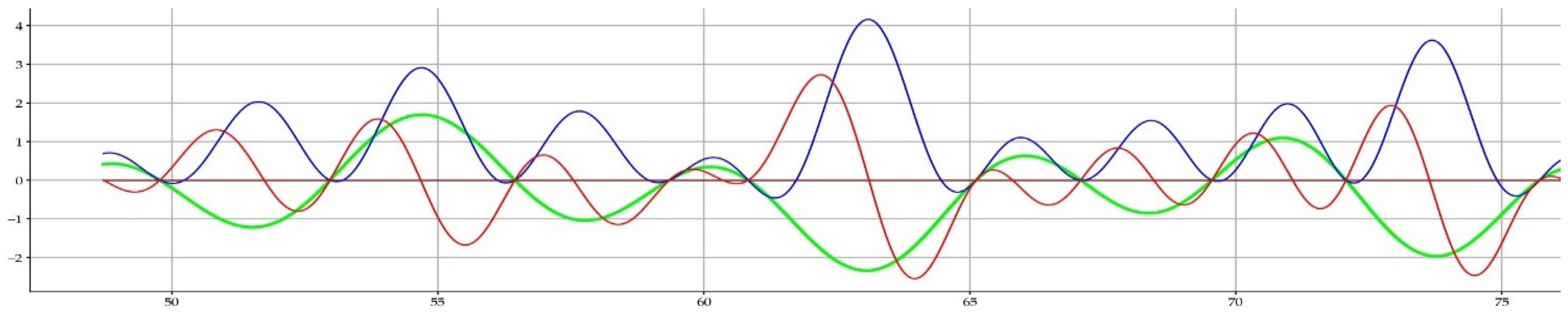
• On the infinite field, the zeros of the $\zeta$ function correspond to the zeros of the real surface of $F$ on the plane of symmetry. The holomorphy is the smoothness property which mitigates and constrains the local variations of the $F$ function. The congruence appears on the anamorphic $\widetilde{ℂ}$ space: $\zeta$ and $F$ include undulations over unit and double periods over the unitary interval $I_n$ corresponding to the nth zero whose midpoint has the ordinate $2\pi \left(n-2+⅝\right)/W\left(\left(n-2+⅝\right)/e\right)$.
• On the finite field, the number of rational points on a smooth curve corresponds to the number of times that the curve meets, up to congruence, the crossings of the grid drawn on a sheet of checkered paper according to the scale of algebraic integers. The rigidity of the irreducible polynomial makes it possible to control the contours of the curve. However, the composition of the Taylor function $F\left(x,y\right)$ with the introduction of the congruence and the constraints of the irreducible polynomial $P\left(x,y\right)$ is more problematic to define and to conceive.

5. Conclusions

In summary, we review the skeleton of the reasoning which has been presented (Figure 16), by highlighting the most significant components. The logical raison d’être is rooted in the contribution of the $S$ function of the poles $p_h$ and zeros $z_n$ of the $F$ function resulting from the $ℱℰ$ of the $\zeta$ function:

$$S\left(s\right)=-𝒫\left(s\right)+\mathcal{Z}\left(s\right)=-{\displaystyle \sum }_{h=0,1}{\left(s-p_h\right)}^{-1}+{\displaystyle \sum }_{n\in \mathbb{N}}{\left(s-z_n\right)}^{-1}$$

Figure 16. Milestones of the article from both the analytical and numerical methods.

Apart from the subset $K$ of trivial zeros $z_k=-2k;k\in \mathbb{N}$, the $N$ non-trivial zeros $z_n$ of the $\zeta$ function belong to the CL $ℒ$ and potentially to the CS $\mathcal{S}\backslash ℒ$. It is necessary, in any calculations, to separate the two disjoint subsets $\mathcal{Z}$ and $ℨ$ of the $N=P+Q$ non-trivial zeros. It is unknown whether the number $Q$ of possible zeros in the CS, excluding the CL, is zero, finite, or infinite.

$$\begin{gathered} \forall z_m\in ℂ:\zeta \left(z_m\right)=0;\left(z_m=z_k\in K\right) \oplus \left(z_m=z_n\in \mathcal{Z}{\displaystyle \cup }ℨ\right) \\ \#\left\{z_n\right\}=\#\left\{Ker\left(\zeta \right)-K\right\}=N \\ \forall {𝓈}_p\in \mathcal{Z}\subset ℒ\subset \mathcal{S}\subset ℂ:\zeta \left({𝓈}_p\right)=0;\#\mathcal{Z}=P={\aleph }_0 \\ \forall s_q\in ℨ\subset \mathcal{S}\backslash ℒ\subset ℂ:\zeta \left(s_q\right)=0;\#ℨ=Q; Q\in \left\{0, 1,\dots , n,\dots ,\infty \right\} \end{gathered}$$

We make use of the fact that the non-trivial zeros of the $\zeta$ function, and those of the $F$ function, taken from the $ℱℰ$, are identical on $ℂ\backslash \left\{0,1\right\}$. It is more effective to focus on this $F$ function, due to its homogeneous form. The $ℱℰ$, in the CS, is written:

$$\begin{gathered} \forall s\in \mathcal{S}≔\left\{0\le x\le 1;s\ne 0;s\ne 1\right\};\widehat{s}=1-s: F\left(s\right)=\frac{\Gamma \left(s/2\right)}{{\pi }^{s/2}}\zeta \left(s\right)=F\left(\widehat{s}\right) \\ \forall s=x+iy\in \mathcal{S};0<x<1: \Gamma \left(s\right) \not\equiv 0;{ e}^s \not\equiv 0 \\ 0<x<1\Rightarrow Ker\left(F\right)\equiv Ker\left(\zeta \right);F\left(s\right)=0\iff \zeta \left(s\right)=0 \end{gathered}$$

The logarithmic derivative of the $F$ function is equal to the poles and zeros function $S$, inspired by Weierstraß’s factorization theorem.

$$\forall s\in ℂ; F\left(s\right)\ne 0: \frac{d\left(lnF\left(s\right)\right)}{ds}=\frac{F^{\prime }\left(s\right)}{F\left(s\right)}=S\left(s\right)=-𝒫\left(s\right)+\mathcal{Z}\left(s\right)=-{\displaystyle \sum }_{Poles}{\left(s-p_h\right)}^{-1}+{\displaystyle \sum }_{Zeros}{\left(s-z_n\right)}^{-1}$$

We also define the family of composite functions in powers of the rational fractions of this $S$ function:

$$\forall m\in \mathbb{N}, \forall s\in ℂ\backslash \left\{poles, Zeros\right\}:{ S}_m\left(s\right)=-{\displaystyle \sum }_{poles}{\left(s-p_h\right)}^{-m}+{\displaystyle \sum }_{Zeros}{\left(s-z_n\right)}^{-m}$$

The successive derivatives $F^{\left(n\right)}$ of $F$ appear as the product of the initial $F$ function and a factor $T_n$: $\forall n\in \mathbb{N},\forall s\in ℂ:F^{\left(n\right)}\left(s\right)=F\left(s\right)T_n\left(s\right)$. The general term $T_n$, of order $n$, is a linear combination of various terms $S_m$:

$$T_n\left(s\right)={\displaystyle \sum }_{p=1,q=2,r=3}^n\left({\lambda }_{p,q,r}^{{\alpha }_p,{\beta }_q,{\gamma }_r}{S}_p^{{\alpha }_p}{S}_q^{{\beta }_q}{S}_r^{{\gamma }_r}\right);\lambda \in \mathbb{Z};r>q>p; n={p\alpha }_p+{q\beta }_q+{r\gamma }_r$$

For $x=½$, $F^{\left(n\right)}$ has both real and imaginary components, which cancel each other out alternately.

$$\forall n\in \mathbb{N},\forall 𝓈\in ℒ,\forall p 𝓈\ne {𝓈}_p :F^{\left(2n\right)}(𝓈)=a_{2n}+i\times 0\in ℝ; F^{\left(2n+1\right)}(𝓈)=0+{ib}_{2n+1}\in iℝ$$

As the $F$ function is holomorphic, its Taylor series makes it possible to calculate the value $F\left(s\right)$ at a point $Z=s$ of the CS $\mathcal{S}$ in the vicinity of a point $H=𝓈$ of the CL $ℒ$, provided that $Z$ and $H$ are close ($\left|\right|Z-H\left|\right|<\epsilon$). This is the direct numerical method. The Taylor expansion of the $F$ function, of a point $s$ in the CS from a point $𝓈$ on the CL is:

$$\forall s=x+{iy}_1\in \mathcal{S}, \forall 𝓈=\text{½}+{iy}_2\in ℒ; \forall p 𝓈\ne {𝓈}_p: F\left(s\right)=F(𝓈)\left(1+{{\displaystyle \sum }}_{n=1}^{\infty }\frac{{\left(\Delta s\right)}^n}{n!}{T}_n(𝓈)\right)$$

If the points $Z$ and $H$ have the same y-coordinate, the expression is simplified:

$$\begin{gathered} F\left(s\right)=F(𝓈)\left(A+iB\right); A={{\displaystyle \sum }}_{n=0}^{\infty }\frac{\dot{x}{}^{2n}}{\left(2n\right)!}{a}_{2n};B={{\displaystyle \sum }}_{n=0}^{\infty }\frac{{\dot{x}}^{2n+1}}{\left(2n+1\right)!}{b}_{2n+1};F(𝓈),A, B,{ a}_{2n},{ b}_{2n+1}\in ℝ \\ F\left(s\right)=F(𝓈)e^{i\theta }\left(1+{a\dot{x}}^2+{i b\dot{x}}^3\right);i\theta ={\dot{x}S}_1=\dot{x}{F}^{\prime }(𝓈)/F(𝓈);\dot{x}=x-\text{½};F(𝓈),\theta ,a>0, b\in ℝ \\ \dot{x}\ne 0; F(𝓈)\ne 0;\left|1+{a\dot{x}}^2+{i b\dot{x}}^3\right|>1\Rightarrow \left|F\left(s\right)\right|>\left|F(𝓈)\right|>0 \end{gathered}$$

However, we must still resolve the particular teratological case where $s=s_q\in \mathcal{S}$ would be in line with a zero $𝓈={𝓈}_p\in ℒ$ on the CL. The same reasoning applies, except that Taylor’s formula is:

$$\begin{gathered} s_q=x+{iy}_q; 𝓈={𝓈}_p=\text{½}+{iy}_p;y_q=y_p;\dot{x}=s_q-{𝓈}_p=x-\text{½};\zeta \left({𝓈}_p\right)=0\Rightarrow F\left({𝓈}_p\right)=0 \\ F\left(s_q\right)=G\left({𝓈}_p\right)\left(e^{i\theta }\left(1-{\dot{x}}^{2}a+{i\dot{x}}^3 b\right)-1\right) \\ G\left({𝓈}_p\right)=\Gamma \left(\text{½}{𝓈}_p\right)/{\pi }^{\text{½}{𝓈}_p}\ne 0;e^{i\theta }\left(1-{\dot{x}}^{2}a+{i\dot{x}}^3 b\right)\ne 1\Rightarrow F\left(s_q\right)\ne 0 \end{gathered}$$

Independently of the $\zeta$ function, this reasoning can be generalized to any meromorphic function, since the argumentation is based on the continuity and differentiability of a holomorphic function and on the decomposition of Weierstraß’s canonical form.

In this article, we elevate the status of the $F$ function, adapted to examine the geometry and the behavior of the $\zeta$ function, both for infinite and finite fields. We reevaluate its strength as an analysis tool compared to that of the $\zeta$ function, because of its balanced geometric shape. Its holomorphic qualities, around the line $x=½$ make it possible to more easily apprehend the symmetry of the $\zeta$ function and to estimate more precisely the values of the $F$ function in the CS.

For the RH, it remains to find a common base to weld together concepts on finite sets and infinite sets. The Jacobi–Weierstraß elliptical functions already constitute a common framework in order to reconcile the paths of both types of sets and to draw a unique perspective.

As a final conclusion, we have analytically and numerically illustrated the RH by the power series of the entire function $F$, in a form resulting from the expression of Hadamard’s product formula. The series expansion of the function $F$ allows the calculation of the values of the function $F$ in the CS, from the values of the function $F$ on the CL, by the Taylor formula of the holomorphic function. This function does not cancel out in the CS\CL. We have exploited a well-known mathematical property of analytical functions, which is not sufficiently utilized in practical applications of the behavior of functions:

• A function of class $C^{\infty }$ has an important property of regularity, but it is a local property.
• An analytical function is more rigid than a function of class $C^{\infty }$. The knowledge of an analytical function in the neighborhood of a point makes it possible to deliver information beyond the neighborhood of this point, in particular for a meromorphic function with isolated zeros and an analytical expansion, making use of Weierstraß’s results.

The function $F$ (like the function $\zeta$), which is meromorphic (at the same time, of class $C^{\infty }$ and analytical) and which integrates this stiffness property, thus allowed us to decipher and exploit its behavior in the narrow ribbon of the CS, starting from its median line, in order to deduce information on the behavior of the $\zeta$ function and its zeros.

References

- Riemann, B. Über die Anzahl der Primzahlen unter Einer Gegebenen Größe; Monatsberichte der Königlichen Preußische Akademie der Wissenschaften: Berlin, Germany, 1859; pp. 671–680. [Google Scholar]
- Hadamard, J. Sur les Zéros de la Fonction ζ(s) de Riemann. Comptes Rendus L’académie Sci. 1896, 122, 1470–1473. [Google Scholar]
- De la Vallée Poussin, C.-J. Recherches analytiques sur la théorie des nombres premiers. Ann. Soc. Sci. 1896, 20–21B, 183–256, 281–352, 363–397, 351–368. [Google Scholar]
- Titchmarsh, E.C. The Theory of the Riemann Zeta-Function, 1st ed.; Oxford University Press: Oxford, UK, 1951; p. 346. [Google Scholar]
- Gram, J.-P. Note sur les zéros de la fonction ζ(s) de Riemann. Acta Math 1903, 27, 289–304. [Google Scholar] [CrossRef]
- Landau, E. Über die Nullstellen der Zeta-funktion. Math. Ann. 1912, 71, 548–564. [Google Scholar] [CrossRef]
- Hardy, G.H. Sur les zéros de la fonction ζ(s) de Riemann. Comptes Rendus L’académie Sci. 1914, 158, 1012–1014. [Google Scholar]
- Littlewood, J.E. On the zeros of the Riemann zeta-function. Proc. Camb. Phil. Soc. 1924, 22, 295–318. [Google Scholar] [CrossRef]
- Levinson, N. More than one third of zeros of Riemann’s zeta-function are on σ = ½. Adv. Math. 1974, 13, 383–436. [Google Scholar] [CrossRef] [Green Version]
- Conrey, J.B. More than 2/5 of the zeros of the Riemann zeta function are on the critical line. J. Reine Angew. Math. 1989, 399, 1–26. [Google Scholar]
- Hardy, G.H.; Littlewood, J.E. The zeros of Riemann’s zeta function on the critical line. Math. Z. 1921, 10, 283–317. [Google Scholar] [CrossRef] [Green Version]
- Atkinson, F.V. The mean value of the zeta-function on the critical line. Proc. London Math. Soc. 1941, 47, 174–200. [Google Scholar]
- Odlyzko, A. Tables of Zeros of the Riemann Zeta Function. 2002. Available online: http://www.dtc.umn.edu/~odlyzko/zeta_tables/index.html (accessed on 20 October 2021).
- Python: A Programming Language. Available online: https://www.python.org/ (accessed on 20 October 2021).
- The SciPy Ecosystem: Sci. Computing Tools for Python. Available online: https://www.scipy.org/ (accessed on 20 October 2021).
- Matplotlib: A Comprehensive Python Plotting Library. Available online: https://matplotlib.org/ (accessed on 20 October 2021).
- Mpmath: A BSD Licensed Python Library for Real and Complex Floating-Point Arithmetic with Arbitrary Precision. Available online: http://mpmath.org (accessed on 20 October 2021).
- SageMath: A Computer Algebra System with Features Covering Many Aspects of Mathematics. Available online: https://wiki2.org/en/SageMath (accessed on 20 October 2021).
- Weierstraß, K. Zur Theorie der Eindeutigen Analytischen Funktionen; Mathematische Abhandlungen der Königlichen Akademie der Wissenschaften: Berlin, Germany, 1876; pp. 11–60. [Google Scholar]
- Artin, E. Quadratische Körper im Gebiete der höheren Kongruenzen I, II. Math. Z. 1924, 19, 153–246. [Google Scholar] [CrossRef]
- Hasse, H. Theorie der relativ-zyklischen algebraischen Funktionenkörper, insbesondere bei endlichen Konstantenkörper. J. Reine Angew. Math. 1934, 172, 37–54. [Google Scholar]
- Hasse, H. Über die Riemannsche Vermutung in Funktionenkörpern. In Proceedings of the Congrès International des Mathématiciens, Oslo, Norway, 13–18 July 1936; pp. 183–206. [Google Scholar]
- Weil, A. Foundations of Algebraic Geometry; American Mathematical Society: Providence, RI, USA, 1946. [Google Scholar]
- Deligne, P. La conjecture de Weil, I. Inst. Hautes Etudes Sci. Publ. Math. 1974, 43, 273–307. [Google Scholar] [CrossRef]
- Deligne, P. La conjecture de Weil, II. Inst. Hautes Etudes Sci. Publ. Math. 1980, 52, 137–252. [Google Scholar] [CrossRef]
- Riguidel, M. Morphogenesis of the Zeta Function in the Critical Strip by Computational Approach. Mathematics 2018, 6, 285. [Google Scholar] [CrossRef] [Green Version]
- Riguidel, M. Numerical Calculations to Grasp a Mathematical Issue Such as the Riemann Hypothesis. Information 2020, 11, 237. [Google Scholar] [CrossRef]
- Riguidel, M. The Two-Layer Hierarchical Distribution Model of Zeros of Riemann’s Zeta Function along the Critical Line. Information 2021, 12, 22. [Google Scholar] [CrossRef]
- Jacobi, C.G.J. Fundamenta Nova Theoriae Functionum Ellipticarum; Univ. Regiom.: Königsberg, Prussia, 1829; (In Latin). Reprinted by Cambridge University Press: Cambridge, UK, 2012. [Google Scholar]
- Tricomi, F.G. Sulle funzioni ipergeometriche confluenti. Ann. Mat. Pura Appl. 1947, 26, 141–175. [Google Scholar] [CrossRef]
- Tricomi, F.G. Funzioni Ipergeometriche Confluenti; Edizioni Cremonese; Consiglio Nazionale Delle Ricerche Monografie Matematiche: Rome, Italy, 1954; ISBN 978-88-7083-449-9. (In Italian) [Google Scholar]
- Temme, N.M. A Set of Algorithms for the Incomplete Gamma Functions. In Probability in the Engineering and Informational Sciences; Cambridge University Press: Cambridge, UK, 1994; Volume 8, pp. 291–307. [Google Scholar]
- Kummer, E.E. De integralibus quibusdam definitis et seriebus infinitis. J. Für Die Reine Und Angew. Math. 1837, 17, 228–242. (In Italian) [Google Scholar] [CrossRef] [Green Version]
- Serre, J.-P. Sur le nombre des points rationnels d’une courbe algébrique sur un corps fini. C. R. Acad. Sci. Paris 1983, 296, 397–402. [Google Scholar]
- Katz, N.M.; Messing, W. Some consequences of the Riemann hypothesis for varieties over finite fields. Invent. Math. 1974, 23, 73–77. [Google Scholar] [CrossRef]
Publisher’s Note: MDPI stays neutral with regard to jurisdictional claims in published maps and institutional affiliations. |
© 2021 by the author. Licensee MDPI, Basel, Switzerland. This article is an open access article distributed under the terms and conditions of the Creative Commons Attribution (CC BY) license (https://creativecommons.org/licenses/by/4.0/).