Time-Optimal Gathering under Limited Visibility with One-Axis Agreement

Pavan Poudel; Gokarna Sharma

doi:10.3390/info12110448

and

Department of Computer Science, Kent State University, Kent, OH 44240, USA

^*

Author to whom correspondence should be addressed.

^†

A preliminary version of this article has been published in SSS’17 conference.

Information2021, 12(11), 448;https://doi.org/10.3390/info12110448

This article belongs to the Special Issue Distributed Systems and Mobile Computing

Version Notes

Order Reprints

Abstract

We consider the distributed setting of N autonomous mobile robots that operate in Look-Compute-Move (LCM) cycles following the well-celebrated classic oblivious robots model. We study the fundamental problem of gathering N autonomous robots on a plane, which requires all robots to meet at a single point (or to position within a small area) that is not known beforehand. We consider limited visibility under which robots are only able to see other robots up to a constant Euclidean distance and focus on the time complexity of gathering by robots under limited visibility. There exists an

O (D_{G})

time algorithm for this problem in the fully synchronous setting, assuming that the robots agree on one coordinate axis (say north), where

D_{G}

is the diameter of the visibility graph of the initial configuration. In this article, we provide the first

O (D_{E})

time algorithm for this problem in the asynchronous setting under the same assumption of robots’ agreement with one coordinate axis, where

D_{E}

is the Euclidean distance between farthest-pair of robots in the initial configuration. The runtime of our algorithm is a significant improvement since for any initial configuration of

N \geq 1

robots,

D_{E} \leq D_{G}

, and there exist initial configurations for which

D_{G}

can be quadratic on

D_{E}

, i.e.,

D_{G} = Θ (D_{E}^{2})

. Moreover, our algorithm is asymptotically time-optimal since the trivial time lower bound for this problem is

Ω (D_{E})

.

Keywords:

distributed algorithms; mobile robots; classic oblivious robot model; gathering; time complexity; visibility; connectivity

1. Introduction

In the classic model of distributed computation by mobile robots, also known as the

O B L O T

model, each robot is modeled as a point in the plane [1,2]. The robots are autonomous (no external control), anonymous (no unique identifiers), indistinguishable (no external identifiers), disoriented (no agreement on local coordinate systems and units of distance measures), oblivious (no memory of past computation), and silent (no direct communication and actions are coordinated via only vision and mobility). They execute the same algorithm. Each robot proceeds in Look-Compute-Move (LCM) cycles: when a robot becomes active, it first obtains a snapshot of its surroundings (Look), then computes a destination based on the snapshot (Compute), and then finally moves towards the destination (Move) [2].

We consider the gathering problem in the

O B L O T

model, where starting from any arbitrary (yet connected) initial configuration, all robots are required to meet at a single point (or to position within a small area) that is not known beforehand. Relaxing the requirement to meet at a single point by positioning them within a small area is performed to circumvent the impossibility result of gathering to a point in the asynchronous setting, even for two robots [3]. In fact, the algorithm we designed in this article positions all robots either at a single point not known beforehand or within a unit line segment not known beforehand depending on different conditions. Gathering is one of the most fundamental tasks and a central benchmark problem in distributed mobile robotics [4]. Early studies on gathering in the

O B L O T

model solved it under unlimited visibility, where each robot is assumed to observe (the locations of) all other robots [5], and all the robots are connected to each other. The viewing range defines the maximum possible distance up to which a robot can observe other robots, and the connectivity range defines the maximum possible distance between any two nodes to be connected (i.e., to have an edge between them). Flocchini et al. [6] provided the first algorithm for gathering in the

O B L O T

model under limited visibility, where each robot can observe (the locations of) other robots within a fixed unit distance (viewing range), and each robot is connected to all other robots within that fixed unit distance (connectivity range), i.e., the viewing and connectivity ranges are the same. Subsequently, several algorithms were studied for this problem under different constraints [2,7,8,9,10]. These studies proved the correctness of the algorithms but provided no runtime analysis (except a proof of finite time termination).

The runtime analysis for gathering has been studied relatively recently [11,12,13,14,15]. Degener et al. [11] provided the first algorithm for this problem with runtime

O (N^{2})

in expectation in the fully synchronous setting, where N is the total number of robots. Degener et al. [12] provided an

O (N^{2})

-time algorithm for this problem in a fully synchronous setting. They also showed that, for some initial configurations, their algorithm is essentially tight by providing a matching lower bound of

Ω (N^{2})

. Kempkes et al. [13] provided an

O (O P T log O P T)

-time algorithm for this problem under a slightly different continuous time setting, where

O P T

is the runtime of an optimal algorithm. All the above algorithms assume that both the viewing and connectivity ranges are of (fixed) radius 1. Recently, Cord-Landwehr et al. [14] provided an

O (N)

-time algorithm for this problem for robots positioned on a grid in a fully synchronous setting. In this algorithm, it is assumed that robots have the viewing range of (distance) 20, i.e., each robot can observe other robots within a fixed distance of 20, but the connectivity range is one, i.e., two robots are connected if and only if they are vertical or horizontal neighbors on the grid. Moreover, each robot is assumed to possess memory for remembering a constant number of previous cycles. Recently, Fischer et al. [15] provided an

O (N^{2})

-time algorithm for gathering on a grid in the fully synchronous setting, if the memory is not available, by using the improved viewing range of 7.

The intriguing open question is whether a time-optimal algorithm can be designed for gathering under limited visibility and if possible, under what conditions. We define time optimality as follows: Let G be the visibility graph of an arbitrary initial configuration I of

N \geq 1

robots in a plane. The robots in the system act as nodes of G. There is an edge between any two nodes in G if the distance between these two nodes is at most the connectivity range. Note that, according to the definitions above, the viewing and connectivity ranges may or may not be the same. If each robot is connected to all robots within its viewing range, then the viewing range also serves as the connectivity range; otherwise, the connectivity range is different than the viewing range. In order to solve the gathering problem, G must be connected [2]; G is connected if the robots (or nodes of G) cannot be separated into two subsets such that no robot of the one subset is connected to any robot of the other subset (and vice versa). For example, the authors in [14] used the viewing range 20, but the robots in horizontal or vertical distance of one are connected. Let

D_{G}

be the diameter of G, which is the greatest distance between any pair of nodes in G following the edges of G. Let

D_{E}

be the diameter of the initial configuration I, which is the greatest Euclidean distance between any pair of robots in I. Notice that for any I,

D_{E} \leq D_{G}

, and for some configurations the gap between

D_{G}

and

D_{E}

can be as much as quadratic on

D_{E}

, i.e.,

D_{G} = Θ (D_{E}^{2})

. Figure 1 illustrates these ideas. Therefore, an

O (D_{E})

-time algorithm would be time-optimal for gathering starting from any initial connected configuration, since

Ω (D_{E})

is the trivial time lower bound for robots to meet at a single point (or to position within a small area) starting from any arbitrary initial configuration. Hence, the open question specifically is whether an

O (D_{E})

-time algorithm can be designed for gathering for classic oblivious robots under limited visibility.

Figure 1. An illustration of two initial configuration dependent parameters,

D_{E}

(the Euclidean diameter) and

D_{G}

(the visibility graph diameter), and the relation between them: (a) the diameter

D_{E}

for an initial arbitrary configuration, (b) the visibility graph G with diameter

D_{G}

for the configuration of the left, and (c) an initial configuration showing the quadratic difference between

D_{E}

and

D_{G}

with

D_{G} = Θ (D_{E}^{2})

.

Recently, Izumi et al. [4] made progress towards addressing this open question. Specifically, they presented an

O (D_{G})

-time algorithm for gathering on the plane in a fully synchronous setting under limited visibility with the condition that robots agree on one coordinate axis. They used viewing range of one with an assumption that the visibility graph G remains connected even if the edges with the corresponding distance of greater than

1 - \frac{1}{\sqrt{2}}

are removed from it. The assumption on the visibility graph G in Izumi et al. [4] essentially means that the connectivity range is of radius

1 - \frac{1}{\sqrt{2}}

(different and in fact smaller than the viewing range of one).

There is still a large gap between the

O (D_{G})

time bound of Izumi et al. [4] and the asymptotically optimal

O (D_{E})

time bound, since

D_{G}

can be quadratic on

D_{E}

(Figure 1). This work closes this gap under the same one axis agreement with a slightly modified viewing range of

\sqrt{10}

and the square connectivity range (if we do not explicitly write “square”, then the viewing and connectivity ranges are circular ) of

\sqrt{2}

compared to the viewing range of one and the (circular) connectivity range of

1 - \frac{1}{\sqrt{2}}

in [4] (if we consider the viewing range of one similar to [4], we need the square connectivity range of

1 - \frac{\sqrt{2}}{\sqrt{10}}

, and our algorithm again achieves

O (D_{E})

runtime). Notice that the square connectivity range of distance c means that a robot is connected to all other robots inside or on the boundary of the (axis-aligned) square area with the (diagonal) distance from the robot to each corner of the square c. Notice also that the square connectivity range of

\sqrt{2}

for a robot is equivalent to the

L_{\infty}

-distance of 1 around the robot. Therefore, if we have both the viewing and connectivity ranges of c, then the area they enclose differs if the connectivity range is “square”; otherwise, they enclose the same area. Moreover, in contrast to Izumi et al. [4], which works in the fully synchronous setting, our algorithm works in the asynchronous setting. The algorithm presented by Izumi et al. [4] follows the movements of robots in one direction (either north or east) along

D_{G}

in such a way that in each round, starting from the southmost and westmost robots, each robot moves towards the farthest neighbor within its connectivity range. In our algorithm, robots do not follow

D_{G}

; instead, they gather at a point (or within a small area) that is not known beforehand in

O (D_{E})

rounds. Particularly, in our algorithm, all the robots gather at a single point not known beforehand under both axis agreements and inside a horizontal line segment of length one that is not known beforehand under one axis agreement. A preliminary version of this article has been published in SSS’17 conference [16], and this article extends that version by including many details and proofs that were missing in that version.

Contributions. We focus, in this article, on optimizing runtime for gathering under limited visibility. We consider autonomous, anonymous, indistinguishable, oblivious, and silent point robots (also called swarms) as in the classic

O B L O T

model [2]. Robots agree on the unit of distance measure. The viewing range is

\sqrt{10}

—a robot can see all other robots within the fixed radius of at most distance

\sqrt{10}

. The square connectivity range is

\sqrt{2}

—a robot is connected to all other robots inside or on the boundary of the (axis-aligned)

2 \times 2

-sized square area for which its center is the position of the robot. In a LCM cycle, a robot can move to any position inside or on the square area, including its four corners. The challenge here is that robot movements must not harm swarm connectivity. As in Izumi et al. [4], we assume that robots agree on one coordinate axis (say north), but they may not agree on the other coordinate axis. Moreover, we assume that the robot setting is asynchronous—there is no notion of common time, and robots perform their LCM cycles arbitrarily. Furthermore, we assume that the robot moves are rigid—a robot in motion in each cycle cannot be stopped (by an adversary) before it reaches its destination at that cycle. Additionally, all previous algorithms assume that when two or more robots move to the same location, they are merged and act as a single robot. In this article, we do not have that assumption; in other words, even if robots are located at the same position and activated at different time, the gathering progress is achieved through the (individual) moves of those robots.

In this article, we prove the following result which, to our best knowledge, is the first algorithm for gathering that is asymptotically time-optimal for classic oblivious robots under limited visibility since the trivial time lower bound for gathering under limited visibility starting from any initial configuration of

N \geq 1

robots is

Ω (D_{E})

.

Theorem 1.

For any initial connected configuration of

N \geq 1

robots with the viewing range of

\sqrt{10}

and the square connectivity range of

\sqrt{2}

on a plane, gathering can be solved in

O (D_{E})

time in the asynchronous setting, when robots agree on one coordinate axis.

Notice that, the visibility graph G must be connected, since gathering may not be solvable under limited visibility if G is not connected [2,6]. Our selection of the viewing and (square) connectivity ranges and the assumption of one-axis agreement play an important role in proving Theorem 1. For both viewing and (circular or square) connectivity ranges of one, we conjecture that there is no

O (D_{E})

-time algorithm for gathering of classic oblivious robots in the asynchronous setting, even when robots agree on both coordinate axes. This is because a robot cannot move more than distance one in each LCM cycle to preserve connectivity, and only the end robots can move in each cycle. Therefore, if the robots are connected as shown in Figure 1,

O (D_{G})

time is required to gather them since only end robots can move and the rest cannot. For the viewing and (circular or square) connectivity ranges of constant

> 1

, we conjecture that there is no

O (D_{E})

-time algorithm for gathering of classic oblivious robots if the robots do not agree on any coordinate axis. This is because the robots’ movements become arbitrary as there is no agreement on the coordinate axes. Thus, robots can only gather if they move following the diameter

D_{G}

, which only provides an

O (D_{G})

-time algorithm.

Technique. Let L be the topmost horizontal line so that all the robots of any initial configuration I are either on the positions of line L or south from L. Let

L^{'}

be the line parallel to L at distance one south of L. The main idea behind the algorithm is to make robots of I in the north of

L^{'}

move to the positions of

L^{'}

or south of

L^{'}

in

O (1)

epochs, even under the asynchronous setting, where an epoch is the time interval for all N robots to execute their LCM cycle at least once (the formal definition of epoch is in Section 2). To accomplish this, we classify the moves of robots into three categories: diagonal hops, horizontal hops, and vertical hops. We will show that if all the robots in the north of

L^{'}

make diagonal or vertical hops, they reach

L^{'}

or south of

L^{'}

in one epoch. However, if some of those robots make a horizontal hop, then in two epochs, they reach positions of

L^{'}

or south of

L^{'}

through the subsequent vertical or diagonal hop. We also show that, if some robots in the north of

L^{'}

do not move in the first epoch, then they reach positions of

L^{'}

or south of

L^{'}

through the vertical or diagonal hop by the next two epochs.

Similarly, let

L_{b}

be the bottommost horizontal line (parallel to L) so that the robots of I are either on

L_{b}

or north of

L_{b}

. The main idea is to show that the robots on

L_{b}

do not move south of

L_{b}

forever. Specifically, we show that robots on

L_{b}

wait for all the robots in the north of

L_{b}

so that they meet at distance (at most) D south of

L_{b}

where D is proportional to the horizontal diameter of the initial configuration I. This is achieved by asking robots not to make any diagonal, horizontal, or vertical hops if they see at least a robot in the north at vertical distance 1 (or more) from their positions (i.e., on or outside the connectivity range of the corresponding robot).

Other Related Work. The classic oblivious robots model or the

O B L O T

model has been considered heavily in order to solve a diverse set of problems, such as scattering, gathering, convergence, circle formation, flocking, etc., in distributed mobile robotics. A comprehensive description of the state-of-the-art research on distributed computing by mobile robots can be found in these excellent books [2,17]. Much work on the classic model on these problems does not provide runtime analysis, for example, see papers on gathering in a non-predefined point [5,6,7,18,19]. Pagli et al. [20] considered gathering classic robots to a small area by avoiding collisions between robots. However, they also do not provide runtime analysis. Kirkpatrick et al. [19] studied gathering as a point convergence problem where starting from an arbitrary initial configuration, robots move in such a manner that they reach inside a circle of radius that is at most

ϵ

,

ϵ > 0

. They proposed an algorithm to solve the problem in the k-asynchronous model (i.e., the degree of asynchrony is bounded to k); however, they showed that point convergence is unsolvable in the fully asynchronous model. In this article, we present an algorithm with runtime analysis to solve the gathering problem in the fully asynchronous model by assuming robots agree on one coordinate axis. Bhagat et al. [21] studied the limited visibility model for robots and presented different geometric pattern formation problems under limited visibility.

Gathering on a predefined point has been studied in several papers [22,23,24]. These papers studied gathering in the context of robots with an extent (i.e., fat robots). Applying these algorithms to the classic model solves gathering in

O (D)

time (provided that gathering point is known to robots), where D is the largest distance from any robot to the predefined gathering point. However, the runtime bound is provided only for the grid, and the gathering point is known to robots a priori. Recently, Braun et al. [25] studied the gathering problem in a three-dimensional Euclidean space under limited visibility and presented

O (n^{2})

-time and

O (D_{E} \cdot n^{\frac{3}{2}})

-time algorithms in the fully synchronous and continuous time models, respectively.

The question of gathering on graphs instead of gathering in the plane was studied in [26,27,28]. Di Stefano and Navarra [27] assumed unlimited visibility and an asynchronous setting and proved the optimal bounds on the number of robot movements for special graph topologies such as trees and rings. D’Angelo et al. [28] showed that gathering can be solved in grids without multiplicity detection. Di Stefano and Navarra [26] extended the results of [28] to infinite grids and bounded the total number of robot movements.

Gathering is solved by circumventing the impossibility of gathering at a single point in some recent papers. The relaxation is on the gathering requirement: Gathering occurs within a small area instead of at a point. A prominent paper that solves gathering in a small area is written by Cord-Landwehr et al. [14] in which, starting from any arbitrary configuration on a grid, robots gathered within a

2 \times 2

-sized grid area. Cord-Landwehr et al. [29] provided an

O (N)

-time algorithm for the robot convergence problem (converging toward a single not predefined point) [30].

Izumi et al. [31] considered the robot scattering problem (opposite of gathering) in the semi-synchronous setting and provided an expected

O (min {N, D^{2} + log N})

-time algorithm; here, D is the diameter of the initial configuration.

All the previous algorithms, including Izumi et al. [4], work in the fully synchronous setting, except for [11] which works in the one-by-one activation setting (also known as sequential activation). Our algorithm works in the asynchronous setting. Furthermore, all previous algorithms assume that when two or more robots move to the same location, they are merged as only one robot. Our algorithm does not merge robots; in other words, even if robots located at the same position are activated at different times, the gathering progress is achieved through the (individual) moves of those robots.

Roadmap. In Section 2, we detail the model and touch on some preliminaries. For the sake of simplicity in discussion, we first provide an

O (D_{E})

-time algorithm for robots on a grid agreeing on both the coordinate axes in Section 3. We then provide an

O (D_{E})

-algorithm for robots on a plane agreeing on both the coordinate axes in Section 4. In Section 5, we discuss how the algorithms of Section 3 and Section 4 can be modified to solve gathering when robots agree on only one axis. Finally, we provide concluding remarks in Section 6 with a brief discussion.

2. Model and Preliminaries

Robots. We consider a distributed system of N robots (agents) from a set

Q = {r_{0}, r_{1}, \dots, r_{N - 1}}

. Each robot is a (dimensionless) point that can move in an infinite two-dimensional real space

R^{2}

. Throughout this article, we will use a point to refer to a robot as well as its position. We denote by

dist (r_{i}, r_{j})

the distance between two robots

r_{i}, r_{j} \in Q

. Each robot

r_{i}

works under limited visibility and viewing range of each robot is

\sqrt{10}

, i.e., a robot

r_{i}

can see and be visible to another robot

r_{j}

if and only if

dist (r_{i}, r_{j}) \leq \sqrt{10}

. For some cases, e.g., for grid, the viewing range smaller than

\sqrt{10}

is sufficient. We describe what exactly is the viewing range when we describe algorithms in Section 3 and Section 5. The connectivity range of each robot is

\sqrt{2}

following square connectivity, i.e., two robots have an edge between them on G if one robot is inside the (axis-aligned)

2 \times 2

-sized square area formed by the other robot being at its center. The robots agree on the unit of distance measure, i.e., the viewing and connectivity ranges of

\sqrt{10}

and

\sqrt{2}

are the same for each robot

r_{i} \in Q

. The robots also agree on one coordinate axis, north (the assumption of robots agreeing on east is analogous). For the sake of simplicity in discussion, the algorithms in Section 3 and Section 4 assume that robots agree on both coordinate axes. The assumption on both axis agreement is lifted in Section 5.

Look-Compute-Move. Each robot

r_{i}

is either active or inactive. When a robot

r_{i}

becomes active, it performs the “Look-Compute-Move” cycle as follows:

Look: For each robot $r_{j}$ that is within the viewing range of $r_{i}$ , $r_{i}$ can observe the position of $r_{j}$ on the plane. Robot $r_{i}$ also knows its own position;
Compute: In any cycle, robot $r_{i}$ may perform an arbitrary computation using only the positions observed during the “look” portion of that cycle. This includes determination of a (possibly) new position for $r_{i}$ for the start of next cycle;
Move: At the end of the cycle, robot $r_{i}$ moves to its new position.

Robot Activation. In the fully synchronous setting (

FSYNC

), every robot is active in every LCM cycle. In the semi-synchronous setting (

SSYNC

), at least one robot is active, and over an infinite number of LCM cycles, every robot is often infinitely active. In the asynchronous setting (

ASYNC

), there is no common notion of time, and no assumption is made on the number and frequency of LCM cycles in which a robot can be active. The only guarantee is that every robot is active infinitely often. Complying with the

ASYNC

setting, we assume that a robot “wakes up” and performs its Look phase at an instant of time. We also assume that during the Move phase, it moves in a straight line and stops only after reaching its destination point; in other words, the moves are rigid [2].

Runtime. For the

FSYNC

setting, time is measured in rounds. Since a robot in the

SSYNC

and

ASYNC

settings could stay inactive for an indeterminate interval of time, we bound a robot’s inactivity and use the standard notion of epoch to measure runtime. An epoch is the smallest interval of time within which each robot is guaranteed to execute its LCM cycle at least once. Therefore, for the

FSYNC

setting, a round is an epoch. We will use the term “time” generally to mean rounds for the

FSYNC

setting and epochs for the

SSYNC

and

ASYNC

settings.

Square Area. Let

r_{i} \in Q

be a robot positioned at coordinate

(x_{i}, y_{i})

. Let

L_{i}, L_{i}^{'}

, respectively, be the horizontal and vertical lines passing through

r_{i}

. Since

r_{i}

knows north,

r_{i}

can easily compute

L_{i}, L_{i}^{'}

. The square area for

r_{i}

, denoted as

S Q (r_{i})

, is an area of the plane enclosed by four lines

L_{i, t}, L_{i, b}, L_{i, l}, L_{i, r}

with

L_{i, t}, L_{i, b}

being parallel to

L_{i}

(perpendicular to

L_{i}^{'}

) and passes through coordinates

(x_{i}, y_{i} + 1)

and

(x_{i}, y_{i} - 1)

, respectively, and

L_{i, l}, L_{i, r}

is perpendicular to

L_{i}

(parallel to

L_{i}^{'}

) and passes through coordinates

(x_{i} - 1, y_{i})

and

(x_{i} + 1, y_{i})

, respectively. Notice that

S Q (r_{i})

is axis-aligned, and both the height and width of it is two. We denote by

p_{t l}, p_{b l}, p_{b r}, p_{t r}

the intersection points of lines

L_{i, t}

and

L_{i, l}

,

L_{i, b}

and

L_{i, l}

,

L_{i, b}

and

L_{i, r}

, and

L_{i, t}

and

L_{i, r}

, respectively. We can divide

S Q (r_{i})

to four quadrant squares

S Q_{1} (r_{i}), S Q_{2} (r_{i}), S Q_{3} (r_{i})

, and

S Q_{4} (r_{i})

with both heights and widths as one. Let

S Q_{1} (r_{i})

and

S Q_{2} (r_{i})

be at the north of

L_{i}

and

S Q_{3} (r_{i})

and

S Q_{4} (r_{i})

be at the south of

L_{i}

. Moreover, let

S Q_{1} (r_{i})

and

S Q_{3} (r_{i})

be at west of

L_{i}^{'}

and

S Q_{2} (r_{i})

and

S Q_{4} (r_{i})

be at east of

L_{i}^{'}

. We say that the positions of

L_{i}

in

S Q (r_{i})

belong to

S Q_{3} (r_{i})

and

S Q_{4} (r_{i})

. Figure 2a illustrates these ideas.

Figure 2. An illustration of (a) Square Area and (b) Unit Area.

Unit Area. Let

r_{j}, r_{k}

, respectively, be the topmost and leftmost robots among the robots in

S Q (r_{i})

. In some situations, both

r_{j}

and

r_{k}

may be the same robot, and this definition is still valid. Let

L_{T}

be the horizontal line passing through

r_{j}

and

L_{L}

be the vertical line passing through

r_{k}

. Let

L_{B}

be the horizontal line parallel to

L_{T}

, and it is at distance one south of

L_{T}

. Similarly, let

L_{R}

be the vertical line parallel to

L_{L}

and at a distance of one east of

L_{L}

. The unit area for

r_{i}

, denoted as

S Q_{u n i t} (r_{i})

, is an area of the plane inside

S Q (r_{i})

enclosed by lines

L_{L}, L_{T}, L_{R}

, and

L_{B}

. Note that

S Q_{u n i t} (r_{i})

is an (axis-aligned) unit square of both height and width one. We denote by

p_{T L}, p_{B L}, p_{B R}

, and

p_{T R}

the intersection points of lines

L_{T}

and

L_{L}

,

L_{B}

and

L_{L}

,

L_{B}

and

L_{R}

, and

L_{T}

and

L_{R}

, respectively. Figure 2b illustrates the idea of unit area computation.

Visibility Graph and Gathering Configuration. We define the visibility graph of any initial configuration I and gathering configurations as follows.

Definition 1

(Initial Visibility Graph). The visibility graph

G (I) = (Q, E)

of any arbitrary initial configuration I of robots is the graph such that, for any two distinct robots

r_{i}

and

r_{j}

,

(r_{i}, r_{j}) \in E

where

r_{j}

is positioned on or inside

S Q (r_{i})

(or vice-versa).

S Q (*)

provides connectivity for robots with square connectivity range

\sqrt{2}

. The gathering problem may not be solvable under limited visibility if the initial visibility graph

G (I)

is not connected [2,6]. Therefore, we assume that

G (I)

is connected at time

t = 0

. Moreover, any algorithm for gathering must maintain the connectivity of

G (I)

during its execution until a gathering configuration is reached. For the sake of clarity, we denote by

G_{t} (I)

the visibility graph

G (I)

for any time

t \geq 0

.

Definition 2

(Ideal Gathering Configuration). An ideal gathering configuration is one where all robots are at a single point that is not known beforehand.

Definition 3

(Relaxed Gathering Configuration). A relaxed gathering configuration is one where all robots are on a horizontal segment of length 1 unit that is not known beforehand.

The relaxed gathering configuration (Definition 3) is inspired from the recent work of Cord-Landwehr et al. [14], where the authors modified the ideal gathering configuration (Definition 2) to solve gathering on a grid by locating all robots within a

2 \times 2

-sized square area that is not known beforehand. Additionally, Definition 3 helps us to circumvent the impossibility results relative to gathering to a point in the

ASYNC

setting [3], even when

N = 2

, by gathering the robots in a unit horizontal line segment. As an example, consider two robots

r_{i}, r_{j}

at distance 1 apart on a horizontal line working under an

ASYNC

setting. Let

r_{i}

and

r_{j}

activate at the same time and

r_{i}

moves to the position of

r_{j}

and

r_{j}

moves to the position of

r_{i}

as both of them move in the horizontal line. This scenario may repeat infinitely since

r_{i}

and

r_{j}

do not have common agreement on east or west under one-axis agreement on north. By using our square connectivity range

\sqrt{2}

, the viewing range

\sqrt{10}

and one-axis agreement, even when

N = 2

, the robots can reach a horizontal segment of length one unit. The viewing range helps each robot

r_{i}

to see whether there is a robot outside

S Q (r_{i})

and decide whether Definition 3 is reached.

Under both axis agreement, our algorithm provides an ideal gathering configuration (Definition 2). Under one-axis agreement, our algorithm provides a relaxed gathering configuration (Definition 3). Since we focus on runtime, we do not explicitly characterize the configurations that do not achieve Definition 2 under one-axis agreement, but we simply prove that all the configurations (at least) attain Definition 3 in

O (D_{E})

time.

3. $O (D_{E})$ Time Algorithm for the Grid

In this section, we define the grid model that is a restriction imposed on the Euclidean plane. The motivation behind designing an algorithm for this model is that it is simple to understand and easy to analyze. We design and analyze an algorithm without the grid restriction in Section 4. In the grid model, a robot moves on a two-dimensional grid and changes its position to one of its eight horizontal, vertical, or diagonal neighboring grid points. Throughout this section, we assume that robots agree on both coordinate axes, and each robot has the viewing range of two. Moreover, each robot has the square connectivity range of

\sqrt{2}

. We say gathering is performed when the robot configuration satisfies Definition 2.

3.1. The Algorithm

The pseudocode of the algorithm is given in Algorithm 1. Depending on the positions of other robots within its viewing range,

r_{i}

distinguishes diagonal, horizontal, and vertical hops, which we discuss separately below. A robot

r_{i}

hops on one of its neighboring grid points based on the diagonal, horizontal, or vertical pattern that matches the snapshot it takes in the Look phase. Notice that since robots agree on north,

r_{i}

never hops on any of the three neighboring grid points relative to north from its position, i.e.,

r_{i}

hops only to one of its five neighboring grid points on the same horizontal line

L_{i}

or south of

L_{i}

. We will show that this allows achieving a gathering progress in every epoch. Since robot moves are not instantaneous due to the

ASYNC

setting, a robot

r_{i}

also does not move if it observes at least one robot in the north of

L_{i}

inside or on

S Q (r_{i})

. This is crucial for guaranteeing that robots do not move south forever. Robot

r_{i}

terminates when it sees no other robot inside or on

S Q (r_{i})

other than its position.

Diagonal Hops. A diagonal hop takes a robot

r_{i}

to one of the two diagonal neighboring grid points in the south (i.e., either

p_{b r}

or

p_{b l}

). Let

L_{i}

be a horizontal line that passes from the current position of a robot

r_{i}

. Robot

r_{i}

makes a diagonal hop when it sees no robot in

S Q (r_{i})

at the north of

L_{i}

(including the positions of

L_{i}

) and either (i)

r_{i}

sees no other robot in

S Q_{3} (r_{i})

(except at its position) and sees at least one robot on

L_{i, r}

at the south of

L_{i}

or (ii)

r_{i}

sees no other robot in

S Q_{4} (r_{i})

(except at its position) and sees at least one robot on

L_{i, l}

at the south of

L_{i}

. In case (i),

r_{i}

hops on grid point

p_{b r}

, whereas in case (ii), it hops on grid point

p_{b l}

.

In this hop, the robot moves diagonally at a distance of

\sqrt{2}

. Figure 3a,b illustrate diagonal hops.

Figure 3. An illustration of moves made by a robot: (a,b) diagonal hops, (c) horizontal hop, and (d,e) vertical hops. The blue shaded area along the grid lines represents that there is no robot in that area. The outer diamond represents the set of grid points within the viewing range of

r_{i}

in grid (i.e., 2).

Algorithm 1: The algorithm for gathering on a grid (under both axis agreement)
	`/*` `In every LCM cycle, each robot $r_{i}$ does the following when it`
	activates: `*/`
	`/` `Look: /`
1	$(x_{i}, y_{i}) \leftarrow$ current position of robot $r_{i}$ in the grid graph G;
2	$C (r_{i}) \leftarrow$ snapshot of the positions of other robots within the viewing range of $r_{i}$ ;
	`/` `Compute: /`
3	$S Q (r_{i}) \leftarrow$ square area for robot $r_{i}$ ;
4	$L_{i}, L_{i}^{'} \leftarrow$ horizontal and vertical lines passing through $r_{i}$ , respectively;
5	$L_{i, t}, L_{i, b} \leftarrow$ horizontal lines parallel to $L_{i}$ and passing through $(x_{i}, y_{i} + 1)$ and
	$(x_{i}, y_{i} - 1)$ , respectively;
6	$L_{i, r}, L_{i, l} \leftarrow$ vertical lines parallel to $L_{i}^{'}$ and passing through $(x_{i} + 1, y_{i})$ and
	$(x_{i} - 1, y_{i})$ , respectively;
7	$d_{i} \leftarrow$ destination point for $r_{i}$ to move;
8	If $r_{i}$ sees no other robot in any of the neighboring grid points on $S Q (r_{i})$ then
9	$r_{i}$ terminates;
10	Else if $r_{i}$ sees at least a robot in $S Q (r_{i})$ in North of $L_{i}$ then
11	$r_{i}$ keeps waiting; $d_{i} \leftarrow (x_{i}, y_{i})$ ; `//` `do nothing`
	`/` `Check the following two conditions for a diagonal hop. /`
12	Else if $r_{i}$ sees no robot in $S Q (r_{i})$ on or West of $L_{i}^{'}$ (except at its position), and sees
	at least a robot on $L_{i, r}$ that is part of $S Q (r_{i})$ in South of $L_{i}$ then `//Figure 3a`
13	$d_{i} \leftarrow (x_{i} + 1, y_{i} - 1)$ ;
14	Else if $r_{i}$ sees no robot in $S Q (r_{i})$ on or East of $L_{i}^{'}$ (except at its position), and sees
	at least a robot on $L_{i, l}$ that is part of $S Q (r_{i})$ in South of $L_{i}$ then `//Figure 3b`
15	$d_{i} \leftarrow (x_{i} - 1, y_{i} - 1)$ ;
	`/` `Check the following condition for a horizontal hop. /`
16	Else if $r_{i}$ sees at least a robot on $(x_{i} + 1, y_{i})$ and sees no other robot in $S Q (r_{i})$ ,
	except on $L_{i}$ in the East then `//` `Figure 3c`
17	$d_{i} \leftarrow (x_{i} + 1, y_{i})$ ;
18	Else`//` `Check either of the following two conditions for a vertical`
	`hop.`
19	If $r_{i}$ sees no robot in $S Q (r_{i})$ in North of $L_{i}$ and sees at least a robot $r_{j}$ on $L_{i}^{'}$ in
	South in $S Q (r_{i})$ then`//` `Figure 3d`
20	$d_{i} \leftarrow (x_{i}, y_{i} - 1);$
21	Else if $r_{i}$ sees no robot in $S Q (r_{i})$ in North of $L_{i}$ and sees at least one robot each
	on two lines $L_{i, l}$ and $L_{i, r}$ on or South of $L_{i}$ in $S Q (r_{i})$ then `//Figure 3e`
22	$d_{i} \leftarrow (x_{i}, y_{i} - 1)$ ;
	`/` `Move: /`
23	$r_{i}$ moves to $d_{i}$ ;
	`/`Note:*`Each robot reaches a grid point after the completion of a`
	`cycle. But a robot may not necessarily see other robot(s) (which`
	`is/are moving) only at grid points since the robots may perform`
	`their LCM cycles at arbitrary times due to the $ASYNC$ setting.`
	`*/`

Horizontal Hops. A horizontal hop takes

r_{i}

to its neighboring grid point on

L_{i}

in the east. When a robot

r_{i}

sees at least one robot

r_{j}

at its horizontal neighboring grid point (and possibly others on

L_{i}

between

r_{i}

and

r_{j}

) and no other robot in

S Q (r_{i})

,

r_{i}

makes a horizontal hop to the neighboring grid point in the east. Figure 3c illustrates the horizontal hop.

Vertical Hops. A vertical hop always takes

r_{i}

to its neighboring grid point vertically south from it. Robot

r_{i}

makes a vertical hop if either (i) it sees a robot

r_{j}

on

L_{i}^{'}

at the south of

L_{i}

and no other robot in

S Q (r_{i})

at the north of

L_{i}

or (ii) it sees at least one robot each on

L_{i, l}

and

L_{i, r}

or south of

L_{i}

and no other robot in

S Q (r_{i})

at the north of

L_{i}

. Figure 3d illustrates case (i) and Figure 3e illustrates case (ii).

3.2. Analysis of the Algorithm

We first prove the correctness of the algorithm in the sense that the visibility graph

G_{t} (I)

remains connected during execution. We then prove the progress of the algorithm such that after a finite number of epochs, any connected initial configuration converges to an ideal gathering configuration (Definition 2). Let I be any arbitrary initial configuration of robots in

Q

on a grid such that

G_{0} (I)

is connected. Let

S E R (I)

be the axis-aligned smallest enclosing rectangle for the robots in I. Let

D_{Y}

and

D_{X}

, respectively, be the height and width of

S E R (I)

. Let

L_{D_{Y}}, L_{D_{Y} - 1}, \dots, L_{0}

be the horizontal line segments of

S E R (I)

at every 1 unit vertical distance, with

L_{D_{Y}}

being the topmost horizontal line segment and

L_{0}

being the bottommost horizontal line segment. Similarly, let

L_{D_{X}}^{'}, L_{D_{X} - 1}^{'}, \dots, L_{0}^{'}

be the vertical line segments of

S E R (I)

at every one unit horizontal distance, with

L_{D_{X}}^{'}

being the rightmost vertical line segment and

L_{0}^{'}

being the leftmost vertical line segment. Let

L_{S}

be the line parallel to

L_{0}

at distance

\frac{D_{X}}{2}

south of

L_{0}

. Figure 4 illustrates these definitions.

Figure 4. An illustration of an axis-aligned smallest enclosing rectangle

S E R (I)

and the triangular area south of it.

Lemma 1.

Given any initial configuration I such that the visibility graph

G_{0} (I)

is connected, the graph

G_{t} (I)

at any time

t > 0

remains connected.

Proof.

For a robot

r_{i}

, since

G_{0} (I)

is connected, there are robots in at least two out of its eight neighboring grid points, unless

r_{i}

is a leaf node in

G_{0} (I)

in which case there may be a robot in only one out of its eight neighboring grid points. We will show that no matter the moves of

r_{i}

and the robots in its eight neighboring grid points, in the new configuration,

r_{i}

has robots in at least two out of its eight neighboring grid points (unless it is a leaf node in

G_{0} (I)

in which case there will be a robot in one of eight neighboring grid points). This immediately proves this lemma from our definition of connectivity.

Notice that the movements of

r_{i}

are either diagonal, horizontal, or vertical, and

r_{i}

never moves to its three neighboring grid points on

S Q (r_{i})

in the north of

L_{i}

. Furthermore,

r_{i}

does not move when it sees at least one robot

r_{j}

at the north of

L_{i}

or inside

S Q (r_{i})

.

A diagonal hop for

r_{i}

is possible when

r_{i}

sees other robot(s)

r_{j}

only on one of its two diagonal neighboring grid points on

S Q_{3} (r_{i})

or

S Q_{4} (r_{i})

, and

r_{i}

moves to the position of

r_{j}

(since

r_{j}

does not move as

r_{j}

sees

r_{i}

at the north of

L_{j}

until

r_{i}

reaches the position of

r_{j}

). Robot

r_{i}

also makes a diagonal hop when it sees other robot(s)

r_{j}

on either

L_{i, l}

only or

L_{i, r}

only that is part of

S Q (r_{i})

in the south of

L_{i}

. Since

r_{j}

is at the south of

L_{i}

, it must be in transit to the neighboring diagonal grid point of

r_{i}

and

r_{i}

, and

r_{j}

meet together when both of them reach that grid point. If one reaches that grid point before, it waits for the other since there will be at least one robot at the north of the horizontal line for the robot on that grid point until

r_{i}

and

r_{j}

meet.

A horizontal hop for

r_{i}

is possible only when

r_{i}

sees

r_{j}

in the east at the horizontal neighboring grid point (and no other robot inside or on

S Q (r_{i})

except on

L_{i}

in the east). After the movement,

r_{i}

either reaches the position of

r_{j}

(if

r_{j}

does not move) or

r_{i}

and

r_{j}

will be at the two vertical neighboring grid points (if

r_{j}

moves). That is, for

r_{j}

to move,

r_{j}

has to see at least one other robot in addition to

r_{i}

on

L_{i}

or at the south. The connectivity is maintained since

r_{i}

is the endpoint robot (i.e., it has only one neighboring robot), and if

r_{j}

is also the endpoint robot, then there is no third robot in the system; otherwise,

r_{j}

must see a robot

r_{k} \neq r_{i}

in one of its five neighboring grid points on

L_{i}

or south of

L_{i}

.

A vertical hop for

r_{i}

is possible when it sees at least one other robot

r_{j}

on the neighboring grid point that is vertically south of it (and possibly others between

r_{i}

and

r_{j}

), but no robot is observed on or inside

S Q (r_{i})

in the north of

L_{i}

. In this case,

r_{i}

reaches the position of

r_{j}

since

r_{j}

cannot move until there is

r_{i}

in the north.

r_{i}

performs a vertical hop also when it sees at least one robot each on the two vertical lines

L_{i, l}

and

L_{i, r}

on or south of

L_{i}

in

S Q (r_{i})

and no robot in

S Q (r_{i})

in the north of

L_{i}

. Suppose

r_{i}

sees two robots

r_{j}

and

r_{k}

in

S Q (r_{i})

on or south of

L_{i}

such that

r_{j} \in L_{i, l}

and

r_{k} \in L_{i, r}

. After the movement, in this case, the distance between

r_{i}

and one of

r_{j}, r_{k}

is at most

\sqrt{2}

as they will be (at most) at the diagonal neighboring grid points from each other. The lemma is described as follows. □

Lemma 2.

Given any initial configuration I, if all the robots are not at one or two neighboring grid positions on the same horizontal line, the robots on the line segment

L_{D_{Y}}

of

S E R (I)

move to the line segment

L_{D_{Y} - 1}

in at most two epochs.

Proof.

Since

L_{D_{Y}}

is the topmost horizontal line segment, there is no robot in the north of

L_{D_{Y}}

. Moreover, since robots agree on north, the robots at the grid points of

L_{D_{Y}}

never move north of

L_{D_{Y}}

. Therefore, if all the robots at the grid points of

L_{D_{Y}}

make diagonal or vertical hops when they become active, then they will reach the positions of

L_{D_{Y} - 1}

; hence, in at most one epoch, all robots on

L_{D_{Y}}

will be at

L_{D_{Y} - 1}

, even in the

ASYNC

setting. Note that in an epoch, each robot completes its LCM cycle at least once. This means that, in this case, each activated robot at

L_{D_{Y}}

completes its LCM cycle after moving to the position of

L_{D_{Y} - 1}

. Therefore, a robot

r_{i}

on

L_{D_{Y}}

remains at a grid point on

L_{D_{Y}}

if and only if it makes a horizontal move in that epoch. We will show that

r_{i}

either terminates or moves to a position on

L_{D_{Y} - 1}

in the next epoch.

Let

r_{j}

be the robot at the horizontal neighboring grid point that

r_{i}

sees on

L_{D_{Y}}

when it makes a horizontal hop. We have it that

r_{i}

must not have seen any robot on its other seven neighboring grid points or inside of

S Q (r_{i})

(except between

r_{i}

and

r_{j}

on the same horizontal line). When

r_{i}

moves to the position of

r_{j}

, either

r_{j}

is still on

L_{D_{Y}}

or has moved to

L_{D_{Y} - 1}

in the neighboring grid point that is vertically south of

r_{j}

. If

r_{j}

has not moved south, either the execution is still in the first epoch or

r_{j}

does not see any other robot except on or between the positions of

r_{i}

and

r_{j}

in the same horizontal line. If

r_{j}

is still in the first epoch, then

r_{i}

reaches the position of

r_{j}

, and either this horizontal moving scenario repeats with execution still being in the first epoch or

r_{j}

moves south. If

r_{j}

does not see any other robot except on or between the positions of

r_{i}

and

r_{j}

in the same horizontal line,

r_{i}

(and all other robots on

L_{i}

up to

r_{j}

) reaches the position of

r_{j}

, and all of them terminate by achieving the gathering configuration. If

r_{j}

has moved to

L_{D_{Y} - 1}

in the first epoch,

r_{i}

moves to the position of

r_{j}

on

L_{D_{Y} - 1}

when it becomes active next time since

r_{j}

is in the neighboring grid point of

S Q (r_{i})

that is vertically south of it. Therefore, in at most two epochs, all the robots on

L_{D_{Y}}

move to the positions of

L_{D_{Y} - 1}

. □

The following observation is immediate for vertical hops since a vertical hop by a robot takes it to its neighboring grid point vertically south of it. For a horizontal/diagonal hop, this is also true since a robot performing a horizontal/diagonal hop never finds its neighboring robot outside

L_{D_{X}}^{'}

and

L_{0}^{'}

.

Observation 1.

No robot of

S E R (I)

moves to the positions outside of lines

L_{0}^{'}

and

L_{D_{X}}^{'}

during the execution.

Lemma 3.

No robot of

S E R (I)

reaches the south of horizontal line

L_{S}

(Figure 4) during the execution.

Proof.

Let

X : = {r_{0}, \dots, r_{X}}

be the robots on

L_{0}

in the increasing order of their x-coordinates (some of the grid points on

L_{0}

may be empty, and it does not impact our analysis). If all robots

r_{0}, \dots, r_{X}

on set

X

have robots on or inside

S Q (*)

at the north of

L_{0}

, they do not move until those robots at the north of

L_{0}

are moved to

L_{0}

. Therefore, we first assume that only

r_{0}

and

r_{X}

have robots at the north of

L_{0}

inside or on

S Q (r_{0})

and

S Q (r_{X})

, respectively, and

{r_{1}, \dots, r_{X - 1}}

have no such robots at the north of

L_{0}

inside or on their respective

S Q (*)

. Robots

r_{2}, \dots, r_{X - 2}

can move to their neighboring grid points that are vertically south of them in one epoch. This is because they do not see any robot at the north of the horizontal line passing through their positions.

In the second epoch,

r_{2}

and

r_{X - 2}

see

r_{1}

and

r_{X - 1}

, respectively, in the north on their respective

S Q (*)

, and only the robots

r_{3}, \dots, r_{X - 3}

can move to the next line in the south from their current horizontal line. This implies that each robot

r_{i}, 1 \leq i \leq \frac{X}{2}

waits for

r_{i - 1}

since it sees

r_{i - 1}

on the neighboring grid point in the north from their position, and this is also the case for the robots from

r_{\frac{X}{2} + 1}

(from

r_{\frac{X}{2} + 2}

in the even

D_{X}

case) to

r_{X - 1}

. The scenario repeats until the middle robot of

L_{0}

reaches at most

\frac{D_{X}}{2} - 1

distance south from

L_{0}

, if

D_{X}

is an odd number). If

D_{X}

is an even number, two robots

r_{\frac{X}{2}}

and

r_{\frac{X}{2} + 1}

of

L_{0}

reach at most

\frac{D_{X}}{2} - 2

distance south from

L_{0}

.

Now consider the case where either

r_{0}

or

r_{X}

has no robot on the neighboring grid point that is vertically north from it in addition to

r_{1}, \dots, r_{X - 1}

. Notice that at least one of

r_{0}

or

r_{X}

must have a robot at the north to maintain the connectivity of

G_{t} (I)

. Let

r_{0}

be that robot (the case of

r_{X}

is analogous). If

r_{0}

moves first, it moves to the position of

r_{1}

in

L_{0}

performing a horizontal hop. If

r_{1}

moves first,

r_{0}

reaches

r_{1}

at the horizontal line immediately below

L_{0}

performing a diagonal hop. By repeating this, the robots

r_{0}, \dots, r_{\frac{X}{2} - 1}

may reach the position of

r_{\frac{X}{2}}

(the middle robot) at distance

D_{\frac{X}{2}}

south of

L_{0}

(i.e.,

L_{S}

). For the remaining robots

r_{\frac{X}{2}}, \dots, r_{X}

, each robot

r_{X - i}, 1 \leq i \leq \frac{X}{2}

sees

r_{X - i + 1}

in the north on respective

S Q (*)

; thus, the middle robot can reach at most

D_{\frac{X}{2}}

south of

L_{0}

. Therefore, this process again ends up at line

L_{S}

in the worst-case.

During the execution, the robots at the north of

L_{0}

in

S E R (I)

may visit the robots south of

L_{0}

. In that case, the robots at the south of

L_{0}

do not move until they see at least one robot at the north of its position inside

S Q (*)

. If a robot does not see any robots at the north of its position, then it either performs a diagonal hop which never takes it to the south of

L_{S}

or it performs a vertical hop. If it performs a vertical hop, it will perform a horizontal hop in the next epoch, and this never takes it south of

L_{S}

. Therefore, according to the moves of the robots of

L_{0}

, it is easy to see that all the robots in

Q

are within the triangular area (as depicted in Figure 4). □

Lemma 4.

The viewings of two and the square connectivity range of

\sqrt{2}

are sufficient for gathering relative to a grid point (that is not known beforehand) on a grid under both axis agreements.

Proof.

If a robot

r_{i}

sees robots only at the south (vertically below or diagonal), it can simply move towards the south, and when

r_{i}

sees no robot in the south and no robot on horizontal neighboring grid points, it can simply terminate. This is because if there is another robot within its viewing range,

r_{i}

must see it in one of its eight neighboring grid points in order to satisfy connectivity for

G_{t} (I), t > 0,

(Lemma 1) since

G_{0} (t)

satisfies this condition. If

r_{i}

sees a robot

r_{j}

in either of its horizontal neighboring grid points, then

r_{i}

moves to the position of

r_{j}

if

r_{j}

is at its east, and

r_{j}

simply waits for

r_{i}

as it does not perform a horizontal hop to the west or moves vertically south. Even in this case,

r_{i}

sees

r_{j}

. Therefore, if

r_{i}

sees no robot in

S Q (r_{i})

, it can terminate. According to the definition of the connectivity range, the viewing range of two is enough for

r_{i}

to maintain connectivity with any of the eight neighboring grid points. □

The analysis of this section proves the following main result.

Theorem 2.

Given any connected configuration of

N \geq 1

robots with the viewing range of two and the square connectivity range of

\sqrt{2}

on a grid, the robots can gather to a point in

O (D_{E})

epochs in the

ASYNC

setting under both axis agreement.

Proof.

We have from Lemma 1 that

G_{t} (I)

remains connected during the execution. We have from Lemma 2 that all the robots at the topmost horizontal line

L_{D_{Y}}

of

S E R (I)

move to

L_{D_{Y} - 1}

in at most two epochs. Thus, after at most two epochs, Lemma 2 applies again to the robots of

L_{D_{Y} - 1}

, which takes all the robots on

L_{D_{Y} - 1}

to

L_{D_{Y} - 2}

or south in next two epochs. This process continues and all the robots in

S E R (I)

move to line

L_{0}

or south of it in at most

2 \cdot D_{Y}

epochs. These robots will be at one grid point in at most the next

D_{X}

epochs. This is because for every one unit of vertical hop of the robots at the south of

L_{0}

, the width of the positions of robots decreases by two. The width of the positions of robots at

L_{0}

is at most

D_{X}

. Thus, the width of the positions of robots becomes zero at distance

\leq \frac{D_{X}}{2}

south of

L_{0}

. Again, from Lemma 2, it takes at most two epochs to move all the robots one unit south; hence, to move all the robots at

\frac{D_{X}}{2}

distance south of

L_{0}

, it takes at most

D_{X}

epochs. Therefore, the robots can gather in

O (D_{X} + D_{Y})

epochs. We have that

max {D_{X}, D_{Y}} \leq D_{E} \leq \sqrt{2} \cdot max {D_{X}, D_{Y}}

for

S E R (I)

of any initial configuration I. Therefore,

D_{X} + D_{Y} \leq 2 \cdot max {D_{X}, D_{Y}}

; hence,

O (D_{X} + D_{Y}) = O (2 \cdot max {D_{X}, D_{Y}}) = O (D_{E})

. The algorithm terminates (Lemma 4) since if a robot

r_{i}

sees no robot in

S Q (r_{i})

other than its current position, then all the robots of

Q

must be gathered in the current position of

r_{i}

(due to the connectivity guarantee of Lemma 1). □

4. $O (D_{E})$ Time Algorithm for the Euclidean Plane

We discuss here how to solve gathering in a Euclidean plane by removing the restrictions on robot moves imposed on a grid. The viewing range is of

\sqrt{10}

, and the square connectivity range is of

\sqrt{2}

(both measured in Euclidean distance). The robots agree on both coordinate axes.

We say gathering is performed when the robot configuration satisfies the ideal gathering configuration (Definition 2).

4.1. The Algorithm

The pseudocode of the algorithm is provided in Algorithm 2. Depending on the positions of other robots in its viewing range, a robot

r_{i}

can decide to hop on the positions of one of its neighboring quadrants

S Q_{3} (r_{i})

or

S Q_{4} (r_{i})

; we do not allow

r_{i}

to move to the positions north of

L_{i}

. In contrast to grid where robots always move in either unit distances (horizontal and vertical hops) or distance

\sqrt{2}

(diagonal hops), in the Euclidean plane, a robot may move with varying distance of at most one for horizontal and vertical hops and varying distance of at most

\sqrt{2}

for diagonal hops. The main difference (with the grid) is on how robots match patterns to perform diagonal, horizontal, and vertical hops. In contrast to relatively simple matching patterns of robots on a grid, the matching patterns of robots for the Euclidean plane are complex.

4.1.1. Overview of the Patterns

The idea is to resemble the patterns for the Euclidean plane to the respective patterns for the grid. For this purpose, we ask each robot

r_{i}

to compute unit area

S Q_{u n i t} (r_{i})

as defined in Section 2.

S Q_{u n i t} (r_{i})

helps

r_{i}

to decide whether to make a diagonal, horizontal, or vertical hop. If

r_{i}

sees itself or at least one robot in

S Q_{u n i t}

,

(r_{i})

is connected to a robot at the north of

L_{T}

, and it does not move. This guarantees that robots do not move south forever. If the robots in

S Q_{u n i t} (r_{i})

are not connected to any other robot outside of

S Q_{u n i t} (r_{i})

at the west of

L_{R}

(or similarly at the east of

L_{L}

), then

r_{i}

makes a horizontal hop to the east (or similarly to west). If

r_{i}

satisfies the conditions for a horizontal hop, except that there is a robot on point

p_{B R}

(or similarly on

p_{B L}

), and the robots in

S Q_{u n i t} (r_{i})

are in a single diagonal line, then it makes a diagonal hop to

p_{B R}

(or similarly to

p_{B L}

). If the robots in

S Q_{u n i t} (r_{i})

are not connected to any other robot outside of

S Q_{u n i t} (r_{i})

at the north of

L_{B}

but (at least) a robot in

S Q_{u n i t} (r_{i})

is connected to a robot on or south of

L_{B}

and

r_{i}

does not satisfy a condition for a diagonal hop, then

r_{i}

makes a vertical hop. Moreover, if

r_{i}

sees at least one robot on each of its two sides (east and west) at horizontal distance ≥ 2, then it makes a vertical hop. The termination is guaranteed by asking

r_{i}

to check, in every LCM cycle, whether all robots in its viewing range are positioned in

S Q_{u n i t} (r_{i})

(that is,

r_{i}

sees no robot outside

S Q_{u n i t} (r_{i})

). When that is the case,

r_{i}

and the remaining robots in

S Q_{u n i t} (r_{i})

run a special procedure in order to reach a single point (Definition 2) and terminate their computation. Reaching a single point is facilitated for robots by both axis agreement.

Algorithm 2: The algorithm for gathering in the Euclidean plane
	`/*` In every LCM cycle, each robot $r_{i}$ does the following when it become
	activated: `*/`
	`/` Look: `/`
1	$(x_{i}, y_{i}) \leftarrow$ current position of robot $r_{i}$ in the plane;
2	$C (r_{i}) \leftarrow$ snapshot of the positions of other robots within the viewing range of $r_{i}$ ;
	`/` Compute: `/`
3	$S Q (r_{i}) \leftarrow$ square area for robot $r_{i}$ ;
4	$S Q_{u n i t} (r_{i}) \leftarrow$ unit area for $r_{i}$ ;
5	$L_{i}, L_{i}^{'} \leftarrow$ horizontal and vertical lines passing through $r_{i}$ , respectively;
6	$L_{i, t}, L_{i, b}, L_{i, r}, L_{i, l} \leftarrow$ top, bottom, right and left boundary lines of $S Q (r_{i})$ , respectively;
7	$L_{T}, L_{B}, L_{R}, L_{L} \leftarrow$ top, bottom, right and left boundary lines of $S Q_{u n i t} (r_{i})$ , respectively;
8	$d_{i} \leftarrow$ destination point for $r_{i}$ to move;
9	If $r_{i}$ sees no robot outside $S Q_{u n i t} (r_{i})$ then
10	execute the termination procedure;
11	If $r_{i}$ sees a robot $r_{j}$ in $S Q_{u n i t} (r_{i})$ that is connected to other robot in North of $L_{i, t}$ (of $S Q (r_{i})$ )
	then
12	$r_{i}$ does not move; $d_{i} \leftarrow (x_{i}, y_{i})$ ;
	`/` `Conditions for horizontal hops /`
13	Else if there is no robot on $L_{B}$ in the segment of $S Q_{u n i t} (r_{i})$ ∧ no robot in $S Q_{u n i t} (r_{i})$ is
	connected to any other robot in West of $L_{R}$ except the robots in $S Q_{u n i t} (r_{i})$ then
14	set the destination point $d_{i}$ as a point at horizontal distance $1 - L_{i j}$ in East (where $L_{i j}$ is
	the horizontal distance from $r_{i}$ to the leftmost robot $r_{j}$ in $S Q_{u n i t} (r_{i})$ );
	`/` Note:*`If $r_{i}$ be the leftmost robot in $S Q_{u n i t} (r_{i})$ , then it moves`
	`distance 1 horizontally in East. And, if the conditions satisfy`
	`symmetrically, then $r_{i}$ sets as destination point to the position on`
	`$L_{L}$ in West. */`
	`/` `Conditions for diagonal hops /`
15	Else if $r_{i}$ sees at least a robot on the diagonal point $p_{B R}$ ∧ all the robots in $S Q_{u n i t} (r_{i})$ are in
	the diagonal line that passes through $S Q_{4} (r_{i})$ ∧ no robot in $S Q_{u n i t} (r_{i})$ is connected to any
	other robot in the West of $L_{R}$ , except the robots in $S Q_{u n i t} (r_{i})$ then
16	set $d_{i}$ as the diagonal point $p_{B R}$ at distance $\sqrt{2} - L_{i j}$ (where $L_{i j}$ is the distance from $r_{i}$ to
	$r_{j}$ , the topmost and leftmost robot in $S Q_{u n i t} (r_{i})$ );
	`/`Note:*`Here, $p_{B R}$ is the intersection point of $L_{B}$ and $L_{R}$ and $S Q_{4} (r_{i})$`
	is the unit square quadrant of $S Q (r_{i})$ in the South-West region. If $r_{i}$
	be the topmost (leftmost) robot in $S Q_{u n i t} (r_{i})$ , then it moves distance
	$\sqrt{2}$ diagonally to $p_{B R}$ . Moreover, if the above conditions satisfy
	symmetrically, then $r_{i}$ sets as destination point $p_{B L}$ (the
	intersection point of $L_{B}$ and $L_{L}$ ). `*/`
17	Else`//` `Conditions for vertical hops`
18	$S P_{u n i t} (r_{i}) \leftarrow$ unit area in West of $L_{i, l}$ and South of $L_{B}$ ;
19	If $r_{i}$ sees a robot at the intersection point of lines $L_{i}^{'}$ and $L_{B}$ ∨ $r_{i}$ sees at least one robot
	each in both sides (East and West) at horizontal distance $\geq 2$ ∨ ( $r_{i}$ sees a robot on $L_{B}$ of
	$S Q_{u n i t} (r_{i})$ , no robot in $S Q_{u n i t} (r_{i})$ is connected to other robot in North of $L_{B}$ and West of
	$L_{L}$ ) ∨ ( $r_{i}$ sees at least one robot in $S Q_{u n i t} (r_{i})$ that is connected to other robot in South of
	$L_{B}$ in West of $L_{R}$ and no robot in $S Q_{u n i t} (r_{i})$ is connected to other robot in North of $L_{B}$
	and West of $L_{L}$ ) ∨ ( $r_{i}$ sees at least a robot in $S P_{u n i t} (r_{i})$ and at least a robot in $S Q_{u n i t} (r_{i})$
	is connected to a robot in North of $L_{B}$ and West of $L_{L}$ ) then
20	set $d_{i}$ as the point vertically South at distance $1 - L_{i j}$ on $L_{B}$ of $S Q_{u n i t} (r_{i})$ (where $L_{i j}$
	is the vertical distance from $r_{i}$ to $L_{T}$ );
	`/` Note:* `If $r_{i}$ be the topmost robot in $S Q_{u n i t} (r_{i})$ then it moves`
	`distance 1 vertically South. */`
	`/` `Move: /`
21	$r_{i}$ moves to $d_{i}$ ;

4.1.2. Detailed Description of the Patterns

We provide details of the patterns below. Robot

r_{i}

terminates when it sees no other robot in

S Q (r_{i})

, except on its current position.

Horizontal Hops. Robot

r_{i}

makes a horizontal hop in the following conditions:

This case is similar to the grid. If $r_{i}$ sees a robot $r_{j}$ at its east at distance one on line $L_{i}$ and there is no robot in $S Q (r_{i})$ , except the current position of $r_{i}$ and possibly on $L_{i}$ from $r_{i}$ up to $r_{j}$ , $r_{i}$ hops to the position of $r_{j}$ (distance 1).
Robot $r_{i}$ hops horizontally east on $L_{i}$ distance $1 - L_{i k}$ ( $L_{i k}$ is the distance between $r_{i}$ and $r_{k}$ , the leftmost robot in $S Q (r_{i})$ ) if all the following conditions are satisfied (Figure 5a illustrates this case for a horizontal hop):

Figure 5. An illustration of a horizontal hop (a) and diagonal hops (b,c).

-
No robot in $S Q_{u n i t} (r_{i})$ is connected to any other robot at the north of $L_{T}$ .
-
No robot in $S Q_{u n i t} (r_{i})$ is connected to any other robot at the west of $L_{R}$ , except for the robots in $S Q_{u n i t} (r_{i})$ .
-
There is no robot on $L_{B}$ of $S Q_{u n i t} (r_{i})$ .

Since we ask the robots to always move east in a horizontal hop, we do not have a symmetric case for horizontal hops under both axis agreements.

Diagonal Hops. Robot

r_{i}

makes a diagonal hop in either of the following conditions:

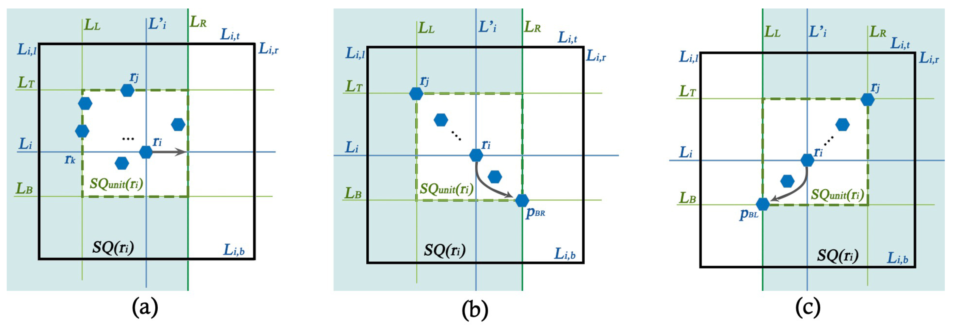
This case is similar to grid. If $r_{i}$ sees no other robot in $S Q (r_{i})$ except at least one robot $r_{j}$ in $S Q_{4} (r_{i})$ on the diagonal corner point $p_{b r}$ , $r_{i}$ hops to $p_{b r}$ . Robot $r_{i}$ moves at a distance of exactly $\sqrt{2}$ if it performs this hop.
Robot $r_{i}$ hops diagonally at a distance of $\sqrt{2} - L_{i j}$ (where $L_{i j}$ is the distance between $r_{i}$ and $r_{j}$ , the topmost which is also the leftmost robot of $S Q_{u n i t} (r_{i})$ at point $p_{T L}$ ) to a point in $S Q_{4} (r_{i})$ , if the following conditions are satisfied:
-
No robot in $S Q_{u n i t} (r_{i})$ is connected to any other robot at the north of $L_{T}$ .
-
No robot in $S Q_{u n i t} (r_{i})$ is connected to any other robot at the west of $L_{R}$ , except the robots in $S Q_{u n i t} (r_{i})$ .
-
All robots in $S Q_{u n i t} (r_{i})$ are in the diagonal line that passes through $S Q_{4} (r_{i})$ .
-
There is at least one robot on the diagonal point $p_{B R}$ of $S Q_{u n i t} (r_{i})$ .
Figure 5b illustrates this hop for $r_{i}$ . The symmetric diagonal case moves $r_{i}$ to point $p_{B L}$ which is illustrated in Figure 5c.

Vertical Hops. If no robot in

S Q_{u n i t} (r_{i})

of a robot

r_{i}

is connected to any other robot at the north of

L_{i, t}

(of

S Q (r_{i})

),

r_{i}

makes a vertical hop of distance

1 - L_{i m}

(where

L_{i m}

is the vertical distance from

r_{i}

to line

L_{T}

) in either of the following conditions:

Robot $r_{i}$ sees at least one robot at the intersection point of $L_{i}^{'}$ and $L_{B}$ .
Robot $r_{i}$ sees at least one robot each at both the east and west at horizontal distance $\geq 2$ . Figure 6b illustrates this case.

Figure 6. An illustration of vertical hops. (a) $r_{i}$ sees at least one robot on $L_{B}$ of $S Q_{u n i t} (r_{i})$ . (b) $r_{i}$ sees at least one robot each in both sides east and west at horizontal distance $\geq 2$ . (c) $r_{i}$ does not see any robot at horizontal distance $\geq 2$ in both sides east and west, but at least one in the west of $L_{L}$ (or East of $L_{R}$ ) and is connected to other robot in the south of $L_{B}$ and west of $L_{i, l}$ (or East of $L_{i, r}$ ).
Robot $r_{i}$ sees at least one robot on $L_{B}$ of $S Q_{u n i t} (r_{i})$ , no robot in $S Q_{u n i t} (r_{i})$ is connected to any other robot at the north of $L_{B}$ and west of $L_{L}$ , and the conditions for a diagonal hop are not satisfied for $r_{i}$ . Figure 6a illustrates this case.
Robot $r_{i}$ sees at least one robot in $S Q_{u n i t} (r_{i})$ that is connected to a robot at the south of $L_{B}$ on or west of $L_{R}$ , and no robot in $S Q_{u n i t} (r_{i})$ is connected to any other robot at the north of $L_{B}$ and west of $L_{L}$ . Figure 6a also illustrates this case.
Let $S P_{u n i t} (r_{i})$ be a unit area at the west of $L_{i, l}$ and south of $L_{B}$ with $L_{B}$ being the topmost horizontal line $L_{T}$ of $S P_{u n i t} (r_{i})$ and $L_{i, l}$ being the rightmost vertical line $L_{R}$ of $S P_{u n i t} (r_{i})$ . Robot $r_{i}$ sees that at least one robot in $S Q_{u n i t} (r_{i})$ is connected to a robot at the north of $L_{B}$ and west of $L_{L}$ , $r_{i}$ sees at least one robot in $S P_{u n i t} (r_{i})$ , and the conditions for a horizontal hop are not satisfied. Figure 6c illustrates this case.

Remark 1.

Robot

r_{i}

also makes a vertical hop if the symmetric situations in the last three conditions are satisfied. The above rules infer that the robots move only under certain situations. Robots do not move in all the remaining situations. This process repeats until all robots of

Q

are inside an (axis-aligned)

1 \times 1

-sized square area so that the special procedure for termination, as described in the next paragraph, can be applied.

4.1.3. The Termination Procedure

We will show in the analysis that the diagonal, horizontal, and vertical hops described above position all robots in

Q

in an axis-aligned

1 \times 1

-sized square area, say

S A

. We now discuss how the robots reach a point and terminate. Let

r_{l}

,

r_{b}

, and

r_{r}

be the leftmost, bottommost, and rightmost robots in

S A

. We have that the unit area

S Q_{u n i t} (r_{i})

of each robot

r_{i}

that is in

S A

overlaps. Therefore, if all the robots in

S A

are in a single diagonal line, then

r_{b}

does not move, and all other robots in

S A

make a diagonal hop with their destination as the current position of

r_{b}

. Otherwise, the robots first perform a horizontal hop, as the destination points the positions on the right vertical line

L_{R}

of

S A

. The robots on

L_{R}

do not move until all the robots in

S A

(the same for all robots) are positioned on

L_{R}

. After that, the robots (now on

L_{R}

) perform a vertical hop to the destination, which is the position of the bottom most robot on

L_{R}

, which does not move. Now, since all the robots reach the same position, they terminate in the next epoch.

We have the following immediate observation after all the robots in

Q

are positioned in an axis-aligned

1 \times 1

-sized square area

S A

.

Observation 2.

The robots within an axis-aligned

1 \times 1

-sized square area

S A

are positioned at a single point in at most two epochs.

4.2. Analysis of the Algorithm

We first prove correctness and then progress to providing a guarantee of the algorithm. We use

S E R (I)

and other definitions as in Section 3 except

L_{S}

. Here, we define

L_{S}

as a horizontal line parallel to

L_{0}

at distance

D_{X}

south of

L_{0}

. Figure 7 illustrates these definitions for the algorithm in the Euclidean plane.

Figure 7. Illustration of

S E R (I)

and the triangular area south of it in the Euclidean plane.

Based on the movement of robots in horizontal, diagonal, and vertical hops, the following observation is immediately made. This is because the robots never make a horizontal hop to the west, and the robots making the horizontal hops never reach east of

L_{D_{X}}^{'}

. In the diagonal hops, robots move to the diagonal position that is closer to the other neighboring robots. Since all the robots are inside

L_{0}^{'}

and

L_{D_{X}}^{'}

initially, there is no neighboring robot outside of those lines; hence, the diagonal hops will also be inside

L_{0}^{'}

and

L_{D_{X}}^{'}

. In the vertical hops, robots always move vertically south. Since no robot has reached outside of

L_{0}^{'}

and

L_{D_{X}}^{'}

with the horizontal as well as diagonal hops, this is true with the vertical hop as well.

Observation 3.

No robot of

S E R (I)

moves outside of lines

L_{0}^{'}

and

L_{D_{X}}^{'}

during the execution.

Lemma 5.

Given that

G_{0} (I)

is connected, the visibility graph

G_{t} (I)

at any time

t > 0

remains connected.

Proof.

We extend the proof of Lemma 1. Similarly to the grid, a robot

r_{i}

either does not move or performs either a diagonal, horizontal, or a vertical hop. Note also that

r_{i}

never moves to any position at the north of

L_{i}

. Furthermore,

r_{i}

does not move when it sees at least one robot

r_{j}

on line

L_{i, t}

or at the north of

L_{i, t}

.

First of all, if the robots move as in the grid case, Lemma 1 provides the connectivity proof for

G_{t} (I), t > 0

, starting from connected

G_{0} (I)

. Therefore, we focus only on the cases that are particularly relevant to the Euclidean plane.

A diagonal hop for

r_{i}

is possible only when the robots in

S Q_{u n i t} (r_{i})

are in the diagonal line that passes through

S Q_{4} (r_{i})

and are not connected to any other robot at the west of

L_{R}

besides the robots in

S Q_{u n i t} (r_{i})

(the analogous case of

S Q_{3} (r_{i})

can be handled similarly). Moreover, there is at least one robot at point

p_{B R}

. Robot

r_{i}

then moves to

p_{B R}

. This preserves connectivity for

G_{t} (I)

since the robot at

p_{B R}

must be connected to at least one robot at the east of

L_{R}

if all the robots of

Q

are not inside

S Q_{u n i t} (r_{i})

. Due to the

ASYNC

setting, the robot

r_{j}

at

p_{B R}

may perform its Look phase while

r_{i}

is in transit to

p_{B R}

. Let

t^{'}

be the time at which

r_{j}

performs its Look. Let

r_{i}

be at point p at distance

\sqrt{2} - x

from

p_{B R}

at time t. Let

S Q^{p} (r_{i})

be

S Q (r_{i})

for

r_{i}

when it is at position p. Even in this case,

r_{j}

does not move in a position outside of

S Q^{p} (r_{i})

regardless of whether it performs a horizontal, vertical, or a diagonal hop, preserving connectivity.

A horizontal hop for

r_{i}

is possible only when the robots in

S Q_{u n i t} (r_{i})

are not connected to any other robot at the west of

L_{R}

similarly to the diagonal hop case with only the difference being that there is no robot on

p_{B R}

so that even when all the robots in

S Q_{u n i t} (r_{i})

are in a diagonal line,

r_{i}

cannot perform a diagonal hop. Even in this case, connectivity is preserved since, if the robots move at most the permitted distance, they would have moved in the grid case.

Similarly, in the vertical hop of robot

r_{i}

, if it sees no robot at the north in

S Q (r_{i})

, it moves vertically south on

L_{i}^{'}

with a distance of exactly one. If

r_{i}

sees at least one robot

r_{j}

at the north in

S Q (r_{i})

and satisfies the conditions for vertical hopping, it hops

1 - L_{i j}

(where

L_{i j}

is the vertical distance between

r_{i}

and

r_{j}

) distance south to a position on

L_{B}

(of

S Q_{u n i t} (r_{i})

). In both cases, by the end of first epoch, each robot moves at most a distance of one toward the south, and the robots remain connected because

r_{i}

reaches at most

\sqrt{2}

distance away from the neighbor robot in

S Q (r_{i})

(if the neighbor robot does not move in this epoch) and remains connected. Moreover, the robots connected to

r_{i}

at the south of

L_{B}

do not move as they find

r_{i}

at the north and the connectivity with them remains unaffected. Thus,

G_{t} (I), t > 0

remains connected with a vertical hop. Figure 8 illustrates the movement of robots and how the connectivity is preserved. Note here that regardless of the grid case where robots are positioned on the grid points, in the Euclidean plane, robots can be positioned anywhere in the plane. The shaded regions in Figure 8 represent the arbitrary positions of robots within the equivalent grid areas in the Euclidean plane. □

Figure 8. An illustration of movements of robots in the Euclidean plane below

L_{0}

. The horizontal and vertical lines are separated by 1 unit distance away, and the robots are positioned arbitrarily in the shaded regions (i.e., they do not need to be necessarily always on the horizontal or vertical lines as in the grid case). At every one unit south of

L_{0}

, the width of the positions of robots decreases by 1 unit; hence, all the robots reach inside a unit square at most

D_{X}

unit south of

L_{0}

. (i) All the robots reached South of

L_{0}

. (ii–xi) Movements of robots in the South of

L_{0}

in each round. (xii) Robots gathered inside a unit square area in the South of

L_{0}

.

Lemma 6.

All the robots in at the north of

L_{D_{Y} - 1}

in

S E R (I)

move to the positions on

L_{D_{Y} - 1}

or south of

L_{D_{Y} - 1}

in at most three epochs.

Proof.

Since

L_{D_{Y}}

is the topmost horizontal line segment of

S E R (I)

, there is no robot at the north of

L_{D_{Y}}

. Moreover, since robots agree on north, they never move to the north of the horizontal line they are currently positioned. Consider the robots in the corridor area

C A

of

S E R (I)

formed by horizontal lines

L_{D_{Y}}

and

L_{D_{Y} - 1}

, excluding the positions of

L_{D_{Y} - 1}

. Note that in the grid case, the robots were either on

L_{D_{Y}}

or on

L_{D_{Y} - 1}

, and we proved in Lemma 2 that the robots on

L_{D_{Y}}

reach

L_{D_{Y} - 1}

or the south in at most two epochs.

Consider

S Q_{u n i t} (r_{i})

of any robot

r_{i}

in

C A

. We will show that all the robots in

S Q_{u n i t} (r_{i})

that are in

C A

reach

L_{D_{Y} - 1}

or below in at most two epochs. Since these robots do not see any robot on or north of

L_{D_{Y}}

, they perform at least one kind of hop (vertical, horizontal, or diagonal) in the first epoch except the robots positioned between

L_{1}^{'}

and

L_{2}^{'}

in the west and

L_{D_{X} - 2}^{'}

and

L_{D_{X} - 1}^{'}

in the east in CA (Figure 8). The robots between

L_{1}^{'}

and

L_{2}^{'}

and

L_{D_{X} - 2}^{'}

and

L_{D_{X} - 1}^{'}

may not satisfy any conditions for movement in the first epoch. If all the robots in

S Q_{u n i t} (r_{i})

in

C A

perform either a diagonal or a vertical hop, they reach

L_{D_{Y} - 1}

or south in one epoch because, with both the diagonal and vertical hops, robots in

S Q_{u n i t} (r_{i})

reach

L_{B}

or below

L_{B}

and

L_{B}

is either

L_{D_{Y} - 1}

or below. If some robots perform a horizontal hop in the first epoch, we show that it performs either a vertical or a diagonal hop in the second epoch.

A robot makes a horizontal hop if it sees no other robot at the west of

L_{R}

, except the robots in

S Q_{u n i t} (r_{i})

, and there is no robot on

L_{B}

of

S Q_{u n i t} (r_{i})

. By the end of the first epoch, all the robots in

S Q_{u n i t} (r_{i})

reach the positions on or east of

L_{R}

if all of them make a horizontal hop. In this case, the robots in CA between

L_{1}^{'}

and

L_{2}^{'}

do not move in the first epoch. If some robots performed horizontal hops and the rest performed vertical/diagonal hops, we only need to guarantee that the robots that performed a horizontal hop on the first epoch reached

L_{B}

or south of it in the second epoch performing a vertical or a diagonal hop. Consider a robot

r_{i}

that satisfies the conditions for a horizontal hop in the first epoch. We have it that there is no robot on

L_{B}

, and the robots in

S Q_{u n i t} (r_{i})

are connected to no other robot besides the robots in

S Q_{u n i t} (r_{i})

at the west of

L_{R}

. Let

S Q_{u n i t}^{E} (r_{i})

be a square area adjacent to

S Q_{u n i t} (r_{i})

at the east between lines

L_{T}

and

L_{B}

. Let

L_{B}^{'}

and

L_{R}^{'}

be the bottom horizontal and right vertical lines of

S Q_{u n i t}^{E} (r_{i})

. If the robots in

S Q_{u n i t}^{E} (r_{i})

are not on

L_{B}^{'}

and not connected to any other robot below

L_{B}^{'}

at the west of

L_{R}^{'}

, they do not move until all the robots in

S Q_{u n i t} (r_{i})

reach

L_{R}

or east of

L_{R}

in

S Q_{u n i t}^{E} (r_{i})

. If there are robots on

L_{B}^{'}

, let x be the robot on

L_{B}^{'}

that is the closest from

L_{R}

. Let

L_{V}

be a line parallel to

L_{R}

at some unit distance west of x. All the robots in

S Q_{u n i t} (r_{i})

at the west of

L_{V}

perform one horizontal move each in the first epoch. The robots on

L_{V}

or east in

S Q_{u n i t} (r_{i})

perform a vertical hop as there are robots on

L_{B}^{'}

. The robots of

S Q_{u n i t} (r_{i})

that performed a horizontal hop on the first epoch now observe robots on

L_{B}

in the second epoch and make a vertical move. Moreover, the robots in

S Q_{u n i t}^{E} (r_{i})

, which were waiting for the robots in

S Q_{u n i t} (r_{i})

to perform a horizontal hop in the first epoch, now see robots at their respective

L_{B}

and, hence, perform either a vertical or a diagonal hop to

L_{B}

. This means that the robots in

C A

between

L_{0}^{'}

and

L_{2}^{'}

also move to

L_{D_{Y} - 1}

or south in two epochs. Arguing similarly, if the robots in

C A

between

L_{D_{X} - 2}^{'}

and

L_{D_{X} - 1}^{'}

do not move in the first epoch, they also see a robot on their respective

L_{B}

in the second epoch since the robots at the west of

L_{D_{X} - 2}^{'}

have already moved south in the first epoch. Thus, these robots also move south in the second epoch. In the same manner the remaining robots between

L_{D_{X} - 1}^{'}

and

L_{D_{X}}^{'}

in

C A

move to

L_{D_{Y} - 1}

or move south in the third epoch as they can observe at least one robot on their respective

L_{B}

. Therefore, in three epochs, all the robots in

C A

reach

L_{D_{Y} - 1}

or south. The Lemma is described follows. □

Lemma 7.

No robots of

S E R (I)

reaches south of

L_{S}

during the execution.

Proof.

We extend the proof of Lemma 3. Let

X : = {r_{0}, \dots, r_{X}}

be the set of robots in the increasing order of their x-coordinates in the corridor area

C A

between

L_{1}

and

L_{0}

of

S E R (I)

. If the robots on set

X

see other robots at distance

\geq 1

north from their positions, they do not move and wait until they do not see any robot at the north at a distance

\geq 1

. Therefore, similarly to Lemma 3, the robots in

C A

that do not see any robot in the north at distance

\geq 1

proceed to move south. This will take those robots to the next corridor

C A^{'}

adjacent to

C A

in the south. Suppose at some time

t > 0

, all the robots reach

C A

between

L_{0}

and

L_{1}

. Some robots might see no robots at the north at the distance

\geq 1

before time t, and they can perform their moves earlier, which does not affect our argument. Now, the robots in

C A

that are in a unit square area (i.e., between

L_{0}^{'}

and

L_{1}^{'}

) in the east perform horizontal moves, and the robots in the next unit square area (i.e., between

L_{1}^{'}

and

L_{2}^{'}

) do not move in the first epoch. Similarly, the robots in

C A

that are in two unit square areas in the west (i.e., between

L_{D_{X} - 2}^{'}

and

L_{D_{X}}^{'}

) do not move in the first epoch. The remaining robots in

C A

between

L_{2}^{'}

and

L_{D_{X} - 2}^{'}

move south. In the next epoch, the robots in

C A

between

L_{1}^{'}

and

L_{2}^{'}

(including the robots that moved horizontally to this area in the previous epoch) move south. The robots in

C A

between

L_{D_{X} - 2}^{'}

and

L_{D_{X} - 1}^{'}

also move south in the this epoch whereas the robots in

C A

between

L_{D_{X} - 1}^{'}

and

L_{D_{X}}^{'}

still do not move; they move in the third epoch. The robots in

C A^{'}

between

L_{2}

and

L_{4}

and

L_{D_{X - 4}}

and

L_{D_{X - 2}}

do not move first, and the other robots move south.

Following this, we can observe that as the robots move to the next corridor (of size one) in the south of

L_{0}

, the width of the positions of robots decreases by one. This is because, at every corridor, the robots in the east most unit square area perform horizontal moves. Therefore, all the robots in

X

will be within a single unit square area in the corridor at distance

D_{X}

south of

L_{0}

(at most). When all the robots are within a unit square area, they follow the termination procedure and do not move further south.

Figure 8 illustrates how the robots move south of

L_{0}

. The figure also shows how the robot chains merge to eventually reach a unit square during execution so that the termination procedure can be executed. □

The following observation is also immediate.

Observation 4.

For every one unit vertical hop of the robots in

Q

in the south of

L_{0}

, the width of the positions of robots decreases by (at least) one.

Lemma 8.

The viewing range of

\sqrt{10}

is sufficient for gathering to a point (that is not known beforehand) on a plane under both axis agreements.

Proof.

Let r be a robot in

Q

.

S Q_{u n i t} (r)

is computed based on the position of other robots in

S Q (r)

, which may lie anywhere within

S Q (r)

. For r to decide whether it is connected to other robots outside

S Q_{u n i t} (r)

, it has to see other robots in both the horizontal and vertical distance of at most one outside

S Q_{u n i t} (r)

. Therefore, the maximum distance between r and some other robot

r^{'}

in

S Q_{u n i t} (r)

(or

S Q (r)

) is

\sqrt{2}

and

r^{'}

may be connected to a robot at a distance of at most

\sqrt{2}

away from

r^{'}

. Therefore, r needs to see at most a distance of

\sqrt{2} + \sqrt{2} = 2 \sqrt{2} = \sqrt{8}

to find out whether there is a robot outside

S Q_{u n i t} (r)

or not. When r sees that no robot in

S Q_{u n i t} (r)

is connected outside of

S Q_{u n i t} (r)

, it can execute the termination procedure.

Now, for the vertical hops, there is one condition that requires r to see at least one robot each at horizontal distance

\geq 2

at both the east and west, within the corridor of

L_{T}

and

L_{B}

. To guarantee whether there is a robot at horizontal distance

\geq 2

or not, r needs to see up to a horizontal distance of

< 3

and vertical distance of

< 1

. This is because if there is any robot at horizontal distance

> 2

, it must be connected to a robot at horizontal distance

< 2

. Therefore, r needs to see at most distance

\sqrt{3^{2} + 1^{2}} = \sqrt{10}

. Figure 9 (left) illustrates this requirement. □

Figure 9. An illustration of the viewing range of

\sqrt{10}

.

The analysis of this section proves the following main result.

Theorem 3.

Given any connected configuration of

N \geq 1

robots with the viewing range of

\sqrt{10}

and the square connectivity range of

\sqrt{2}

on a plane, the robots can gather to a point in

O (D_{E})

epochs in the

ASYNC

setting under both axis agreements.

Proof.

We have from Lemma 5 that, given a connected

G_{0} (I)

,

G_{t} (I), t > 0,

remains connected during the execution of the algorithm. We have from Lemma 6 that all the robots at the topmost horizontal line

L_{D_{Y}}

of

S E R (I)

move to

L_{D_{Y} - 1}

or south of

L_{D_{Y} - 1}

in at most two epochs. In other words,

L_{D_{Y} - 1}

becomes

L_{D_{Y}}

in at most two epochs and Lemma 6 applies again to

L_{D_{Y} - 1}

. Therefore, all the robots in

S E R (I)

move to line

L_{0}

or south of it in at most

2 \cdot D_{Y}

epochs. After that, we have it that, from Lemma 7, these robots will be inside an axis-aligned unit area in at most next

2 \cdot D_{X}

epochs, arguing similarly with respect to Lemma 6. After all the robots of

Q

reach the insides of an unit square area, we have from Observation 2 that they reach a single point in at most the next two epochs. Therefore, the robots gather to a single point in

2 \cdot D_{Y} + 2 \cdot D_{X} + 2 = O (D_{X} + D_{Y}) = O (D_{E})

epochs. The algorithm terminates (Lemma 8). □

5. Gathering under One-Axis Agreement

We discuss modifying the above algorithms when the robots agree on only one axis.

5.1. Grid

We first discuss changes in the model of Section 3. We say gathering is performed when the robot configuration satisfies the relaxed gathering configuration (Definition 3). We also relax the viewing range from 2 to 3.

We now discuss changes in Algorithm 1 (Section 3). The change is only on Rules 1 (termination) and 3 (horizontal hop). Regarding Rule 3, instead of

r_{i}

moving only to the east (Figure 3 (middle)),

r_{i}

can also move to the west as well if it sees no robots on or inside

S Q (r_{i})

, except for the situation where there is exactly one robot

r_{j}

on the neighboring grid point on

L_{i}

in the west. Regarding Rule 1,

r_{i}

terminates if it sees all the robots at at most one unit apart in a horizontal line (i.e., all the robots are positioned in two horizontal neighboring grid points).

Lemma 9.

The viewing range of three is sufficient for gathering on a grid with guaranteed termination under a one-axis agreement.

Proof.

Notice that a robot

r_{i}

terminates if it sees all the robots in

Q

are at most two neighboring grid points (one is current position of

r_{i}

and the other is either the left horizontal grid point only or the right horizontal neighboring grid point only). For

r_{i}

to make a decision that the robots are not at any third grid point, it has to see all the neighboring grid points of its two horizontal neighboring grid points as well. The distance from

r_{i}

to either of its horizontal neighboring grid point is one, and the distance of the neighboring grid points of

r_{i}

’s horizontal neighboring grid points is at most

\sqrt{2}

. Therefore,

r_{i}

needs the viewing range of

(1 + \sqrt{2}) < 3

. The connectivity range remains

\sqrt{2}

. □

Having the viewing range of three, the analysis of the algorithm in Section 3 applies directly to the modified algorithm for the grid under the one axis agreement. Therefore, we summarize the main result in the following theorem.

Theorem 4.

Given any connected configuration of

N \geq 1

robots with the viewing range of three and the square connectivity range of

\sqrt{2}

on a grid, the robots can gather in a unit length horizontal line segment (that is not known beforehand) in

O (D_{E})

epochs in the

ASYNC

setting under a one-axis agreement.

5.2. Euclidean Plane

We first discuss changes in the model of Section 4. We say gathering is performed when the configuration satisfies the relaxed gathering configuration (Definition 3). The viewing and square connectivity ranges remain the same as in Section 4.

We now discuss changes in the algorithm. The change is on horizontal and vertical hops and on termination. Instead of computing

S Q_{u n i t} (r_{i})

using

L_{L}

and

L_{T}

as reference lines,

S Q_{u n i t} (r_{i})

also needs to be computed by using

L_{R}

and

L_{T}

as references. When

r_{i}

sees no other robot on one side (say west) at a distance of >1 but does on the other side (east), it takes the topmost robot

r_{j}

and leftmost robot

r_{k}

in

S Q (r_{i})

in order to compute

S Q_{u n i t} (r_{i})

; for the symmetric case, it takes the topmost and rightmost robots in

S Q (r_{i})

as a reference. This allows the robots to make horizontal hops in both directions (not necessarily only east under both axis agreement). Therefore,

r_{i}

hops to the west of

L_{i}

if the conditions for horizontal hop defined in Section 4 are satisfied symmetrically. Regarding vertical hopping, the following changes are made in the last three conditions:

–: Robot $r_{i}$ sees at least one other robot each on both sides of $L_{i}^{'}$ on $L_{B}$ or south of $L_{B}$ , which is connected to at least one robot of $S Q_{u n i t} (r_{i})$ .
–: Robot $r_{i}$ sees at least one other robot on $L_{B}$ or south of $L_{B}$ (which is connected $S Q_{u n i t} (r_{i})$ ) at one side of $L_{i}^{'}$ (say east) and at least one other robot at horizontal distance ≥2 on the other side (west) (and vice-versa).
–: Robot $r_{i}$ sees other robot(s) on $L_{B}$ (or connected to other robot(s) at the south of $L_{B}$ ) only at one side of $L_{i}^{'}$ , say east, then finds the leftmost robot $r_{l}$ on $L_{B}$ of $S Q_{u n i t} (r_{i})$ (or south of $L_{B}$ that is connected to $S Q_{u n i t} (r_{i})$ ) and sees that no robot in $S Q_{u n i t} (r_{i})$ is connected to another robot at its left (i.e., west) at a horizontal distance of ≥1 from $r_{l}$ (and vice-versa).

Regarding termination,

r_{i}

terminates if all the robots it sees within its viewing range (including itself) are within a horizontal line segment of length 1. We will show in the analysis that, with these changes, the algorithm positions the robots in

Q

inside an axis-aligned

1 \times 1

-sized square area

S A

in

O (D_{E})

epochs.

We now discuss how the robots in

S A

reached a relaxed gathering configuration (Definition 3). Let

r_{b}

be the bottommost robot in

S A

(if more than one, pick one arbitrarily). Let

L_{B}

be the horizontal line passing through

r_{b}

. The robots on

L_{B}

(including

r_{b}

) do not move. The other robots move vertically to the positions of

L_{B}

. The viewing range allows the robots to decide whether there are robots outside

S A

or not.

Proof of Theorem 1:

It is easy to see from the analysis of Section 4 that robots in

Q

reach inside an axis-aligned unit square area in

O (D_{E})

epochs. The only change on the analysis is on horizontal hops, which does not increase the number of epochs for the robots in

Q

to reach the inside of the unit area. Finally, it takes at most one additional epoch for all the robots that are in the unit square area to reach

L_{B}

. The robots that are not on

L_{B}

move vertically to

L_{B}

, and the robots on

L_{B}

do not move. Therefore, the robots reach a relaxed gathering configuration (Definition 3) in

O (D_{E})

epochs. □

6. Concluding Remarks

We have presented, to the best of our knowledge, the first time-optimal

O (D_{E})

-epoch algorithm for gathering

N \geq 1

classic oblivious robots in a plane in the

ASYNC

setting under limited visibility, improving significantly on the previous

O (D_{G})

-round algorithm of [4] that works in the

FSYNC

setting. Our result assumes the viewing range of

\sqrt{10}

, the square connectivity range of

\sqrt{2}

, and the agreement on one axis. This is in contrast to the viewing range of one and the (circular) connectivity range of

1 - \frac{1}{\sqrt{2}}

in [4] under the same one axis agreement. For future work, it will be interesting to relax our assumption of rigid moves to accommodate non-rigid moves. It will also be interesting to reduce the gap between the connectivity and viewing ranges without affecting time complexity.

Author Contributions

Conceptualization, G.S.; methodology, P.P. and G.S.; formal analysis, P.P. and G.S.; investigation, P.P. and G.S.; resources, G.S.; writing—original draft preparation, P.P.; writing—review and editing, G.S.; supervision, G.S.; project administration, G.S. All authors have read and agreed to the published version of the manuscript.

Funding

This research received no external funding.

Acknowledgments

The authors thank Costas Busch for introducing this problem.

Conflicts of Interest

The authors declare no conflict of interest.

References

Suzuki, I.; Yamashita, M. Distributed Anonymous Mobile Robots: Formation of Geometric Patterns. SIAM J. Comput. 1999, 28, 1347–1363. [Google Scholar] [CrossRef] [Green Version]
Flocchini, P.; Prencipe, G.; Santoro, N. Distributed Computing by Oblivious Mobile Robots. Synth. Lect. Distrib. Comput. Theory 2012, 3, 1–185. [Google Scholar] [CrossRef]
Prencipe, G. Impossibility of Gathering by a Set of Autonomous Mobile Robots. Theor. Comput. Sci. 2007, 384, 222–231. [Google Scholar] [CrossRef] [Green Version]
Izumi, T.; Kawabata, Y.; Kitamura, N. Toward Time-Optimal Gathering for Limited Visibility Model. 2015. Available online: https://sites.google.com/site/micromacfrance/abstract-tasuke (accessed on 18 October 2021).
Cieliebak, M.; Flocchini, P.; Prencipe, G.; Santoro, N. Solving the Robots Gathering Problem. In Proceedings of the 30th International Colloquium on Automata, Languages, and Programming, Eindhoven, The Netherlands, 30 June–4 July 2003; pp. 1181–1196. [Google Scholar]
Flocchini, P.; Prencipe, G.; Santoro, N.; Widmayer, P. Gathering of Asynchronous Robots with Limited Visibility. Theor. Comput. Sci. 2005, 337, 147–168. [Google Scholar] [CrossRef] [Green Version]
Prencipe, G. Autonomous Mobile Robots: A Distributed Computing Perspective. In Proceedings of the 9th International Symposium on Algorithms and Experiments for Sensor Systems, Wireless Networks and Distributed Robotics, Sophia Antipolis, France, 5–6 September 2013; pp. 6–21. [Google Scholar]
Souissi, S.; Défago, X.; Yamashita, M. Gathering Asynchronous Mobile Robots with Inaccurate Compasses. In Proceedings of the 10th on Principles of Distributed Systems, Bordeaux, France, 12–15 December 2006; pp. 333–349. [Google Scholar] [CrossRef]
Cieliebak, M.; Flocchini, P.; Prencipe, G.; Santoro, N. Distributed Computing by Mobile Robots: Gathering. SIAM J. Comput. 2012, 41, 829–879. [Google Scholar] [CrossRef] [Green Version]
Agathangelou, C.; Georgiou, C.; Mavronicolas, M. A Distributed Algorithm for Gathering Many Fat Mobile Robots in the Plane. In Proceedings of the 2013 ACM Symposium on Principles of Distributed Computing, Montréal, QC, Canada, 22–24 July 2013; pp. 250–259. [Google Scholar]
Degener, B.; Kempkes, B.; Meyer auf der Heide, F. A Local O(n2) Gathering Algorithm. In Proceedings of the Twenty-Second Annual ACM Symposium on Parallelism in Algorithms and Architectures, Thira, Greece, 13–15 June 2010; pp. 217–223. [Google Scholar]
Degener, B.; Kempkes, B.; Langner, T.; Meyer auf der Heide, F.; Pietrzyk, P.; Wattenhofer, R. A Tight Runtime Bound for Synchronous Gathering of Autonomous Robots with Limited Visibility. In Proceedings of the Twenty-Third Annual ACM Symposium on Parallelism in Algorithms and Architectures, San Jose, CA, USA, 4–6 June 2011; pp. 139–148. [Google Scholar]
Kempkes, B.; Kling, P.; Meyer auf der Heide, F. Optimal and Competitive Runtime Bounds for Continuous, Local Gathering of Mobile Robots. In Proceedings of the Twenty-Fourth Annual ACM Symposium on Parallelism in Algorithms and Architectures, Pittsburgh, PA, USA, 25–27 June 2012; pp. 18–26. [Google Scholar]
Cord-Landwehr, A.; Fischer, M.; Jung, D.; Meyer auf der Heide, F. Asymptotically Optimal Gathering on a Grid. In Proceedings of the 28th ACM Symposium on Parallelism in Algorithms and Architectures, Pacific Grove, CA, USA, 11–13 July 2016; pp. 301–312. [Google Scholar] [CrossRef] [Green Version]
Castenow, J.; Fischer, M.; Harbig, J.; Jung, D.; Meyer auf der Heide, F. Gathering Anonymous, Oblivious Robots on a Grid. Theor. Comput. Sci. 2020, 815, 289–309. [Google Scholar] [CrossRef]
Poudel, P.; Sharma, G. Universally Optimal Gathering Under Limited Visibility; Lecture Notes in Computer Science; Springer: Berlin/Heidelberg, Germany, 2017; Volume 10616, pp. 323–340. [Google Scholar] [CrossRef]
Distributed Computing by Mobile Entities, Current Research in Moving and Computing; Lecture Notes in Computer Science; Flocchini, P.; Prencipe, G.; Santoro, N. (Eds.) Springer: Berlin/Heidelberg, Germany, 2019; Volume 11340. [Google Scholar] [CrossRef]
Ando, H.; Suzuki, I.; Yamashita, M. Formation and Agreement Problems for Synchronous Mobile Robots with Limited Visibility. In Proceedings of the Tenth International Symposium on Intelligent Control, Monterey, CA, USA, 27–29 August 1995; pp. 453–460. [Google Scholar] [CrossRef]
Kirkpatrick, D.; Kostitsyna, I.; Navarra, A.; Prencipe, G.; Santoro, N. Separating Bounded and Unbounded Asynchrony for Autonomous Robots: Point Convergence with Limited Visibility. In Proceedings of the 2021 ACM Symposium on Principles of Distributed Computing; ACM: New York, NY, USA, 2021; pp. 9–19. [Google Scholar] [CrossRef]
Pagli, L.; Prencipe, G.; Viglietta, G. Getting Close Without Touching: Near-gathering for Autonomous Mobile Robots. Distrib. Comput. 2015, 28, 333–349. [Google Scholar] [CrossRef] [Green Version]
Bhagat, S.; Mukhopadhyaya, K.; Mukhopadhyaya, S. Computation Under Restricted Visibility. In Distributed Computing by Mobile Entities: Current Research in Moving and Computing; Springer International Publishing: Cham, Switzerland, 2019; pp. 134–183. [Google Scholar] [CrossRef]
Sharma, G.; Busch, C.; Mukhopadhyay, S.; Malveaux, C. Tight Analysis of a Collisionless Robot Gathering Algorithm. ACM Trans. Auton. Adapt. Syst. 2017, 12, 3:1–3:20. [Google Scholar] [CrossRef]
Lukovszki, T.; auf der Heide, F.M. Fast Collisionless Pattern Formation by Anonymous, Position-Aware Robots. In Proceedings of the 18th Principles of Distributed Systems, Cortina d’Ampezzo, Italy, 16–19 December 2014; pp. 248–262. [Google Scholar]
Cord-Landwehr, A.; Degener, B.; Fischer, M.; Hüllmann, M.; Kempkes, B.; Klaas, A.; Kling, P.; Kurras, S.; Märtens, M.; Meyer auf der Heide, F.; et al. Collisionless Gathering of Robots with an Extent. In Proceedings of the 37th Conference on Current Trends in Theory and Practice of Computer Science, Nový Smokovec, Slovakia, 22–28 January 2011; pp. 178–189. [Google Scholar]
Braun, M.; Castenow, J.; auf der Heide, F.M. Local Gathering of Mobile Robots in Three Dimensions. In SIROCCO; Lecture Notes in Computer Science; Springer: Berlin/Heidelberg, Germany, 2020; Volume 12156, pp. 63–79. [Google Scholar] [CrossRef]
Di Stefano, G.; Navarra, A. Optimal Gathering on Infinite Grids. In Proceedings of the 16th Symposium on Self-Stabilizing Systems, Paderborn, Germany, 28 September–1 October 2014; pp. 211–225. [Google Scholar]
Di Stefano, G.; Navarra, A. Optimal gathering of oblivious robots in anonymous graphs and its application on trees and rings. Distrib. Comput. 2017, 30, 75–86. [Google Scholar] [CrossRef]
D’Angelo, G.; Stefano, G.D.; Klasing, R.; Navarra, A. Gathering of Robots on Anonymous Grids without Multiplicity Detection. In Proceedings of the 19th International Colloquium on Structural Information and Communication Complexity, Reykjavik, Iceland, 30 June–2 July 2012; pp. 327–338. [Google Scholar] [CrossRef] [Green Version]
Cord-Landwehr, A.; Degener, B.; Fischer, M.; Hüllmann, M.; Kempkes, B.; Klaas, A.; Kling, P.; Kurras, S.; Märtens, M.; Meyer auf der Heide, F.; et al. A New Approach for Analyzing Convergence Algorithms for Mobile Robots. In Proceedings of the 38th International Colloquium on Automata, Languages, and Programming, Zurich, Switzerland, 4–8 July 2011; pp. 650–661. [Google Scholar] [CrossRef]
Cohen, R.; Peleg, D. Convergence Properties of the Gravitational Algorithm in Asynchronous Robot Systems. SIAM J. Comput. 2005, 34, 1516–1528. [Google Scholar] [CrossRef]
Izumi, T.; Potop-Butucaru, M.G.; Tixeuil, S. Connectivity-preserving Scattering of Mobile Robots with Limited Visibility. In Proceedings of the 12th Symposium on Self-Stabilizing Systems, New York, NY, USA, 20–22 September 2010; pp. 319–331. [Google Scholar]

Figure 1. An illustration of two initial configuration dependent parameters,

D_{E}

(the Euclidean diameter) and

D_{G}

(the visibility graph diameter), and the relation between them: (a) the diameter

D_{E}

for an initial arbitrary configuration, (b) the visibility graph G with diameter

D_{G}

for the configuration of the left, and (c) an initial configuration showing the quadratic difference between

D_{E}

and

D_{G}

with

D_{G} = Θ (D_{E}^{2})

.

Figure 2. An illustration of (a) Square Area and (b) Unit Area.

Figure 3. An illustration of moves made by a robot: (a,b) diagonal hops, (c) horizontal hop, and (d,e) vertical hops. The blue shaded area along the grid lines represents that there is no robot in that area. The outer diamond represents the set of grid points within the viewing range of

r_{i}

in grid (i.e., 2).

Figure 4. An illustration of an axis-aligned smallest enclosing rectangle

S E R (I)

and the triangular area south of it.

Figure 5. An illustration of a horizontal hop (a) and diagonal hops (b,c).

Figure 6. An illustration of vertical hops. (a)

r_{i}

sees at least one robot on

L_{B}

of

S Q_{u n i t} (r_{i})

. (b)

r_{i}

sees at least one robot each in both sides east and west at horizontal distance

\geq 2

. (c)

r_{i}

does not see any robot at horizontal distance

\geq 2

in both sides east and west, but at least one in the west of

L_{L}

(or East of

L_{R}

) and is connected to other robot in the south of

L_{B}

and west of

L_{i, l}

(or East of

L_{i, r}

).

Figure 7. Illustration of

S E R (I)

and the triangular area south of it in the Euclidean plane.

Figure 8. An illustration of movements of robots in the Euclidean plane below

L_{0}

. The horizontal and vertical lines are separated by 1 unit distance away, and the robots are positioned arbitrarily in the shaded regions (i.e., they do not need to be necessarily always on the horizontal or vertical lines as in the grid case). At every one unit south of

L_{0}

, the width of the positions of robots decreases by 1 unit; hence, all the robots reach inside a unit square at most

D_{X}

unit south of

L_{0}

. (i) All the robots reached South of

L_{0}

. (ii–xi) Movements of robots in the South of

L_{0}

in each round. (xii) Robots gathered inside a unit square area in the South of

L_{0}

.

Figure 9. An illustration of the viewing range of

\sqrt{10}

.

Publisher’s Note: MDPI stays neutral with regard to jurisdictional claims in published maps and institutional affiliations.

© 2021 by the authors. Licensee MDPI, Basel, Switzerland. This article is an open access article distributed under the terms and conditions of the Creative Commons Attribution (CC BY) license (https://creativecommons.org/licenses/by/4.0/).

Time-Optimal Gathering under Limited Visibility with One-Axis Agreement^†

Abstract

1. Introduction

2. Model and Preliminaries

3. $O (D_{E})$ Time Algorithm for the Grid

3.1. The Algorithm

3.2. Analysis of the Algorithm

4. $O (D_{E})$ Time Algorithm for the Euclidean Plane

4.1. The Algorithm

4.1.1. Overview of the Patterns

4.1.2. Detailed Description of the Patterns

4.1.3. The Termination Procedure

4.2. Analysis of the Algorithm

5. Gathering under One-Axis Agreement

5.1. Grid

5.2. Euclidean Plane

6. Concluding Remarks

Author Contributions

Funding

Acknowledgments

Conflicts of Interest

References

Article Metrics

Citations

Article Access Statistics

Time-Optimal Gathering under Limited Visibility with One-Axis Agreement †

Abstract

1. Introduction

2. Model and Preliminaries

3. O ( D E ) Time Algorithm for the Grid

3.1. The Algorithm

3.2. Analysis of the Algorithm

4. O ( D E ) Time Algorithm for the Euclidean Plane

4.1. The Algorithm

4.1.1. Overview of the Patterns

4.1.2. Detailed Description of the Patterns

4.1.3. The Termination Procedure

4.2. Analysis of the Algorithm

5. Gathering under One-Axis Agreement

5.1. Grid

5.2. Euclidean Plane

6. Concluding Remarks

Author Contributions

Funding

Acknowledgments

Conflicts of Interest

References

Article Metrics

Citations

Article Access Statistics

Time-Optimal Gathering under Limited Visibility with One-Axis Agreement^†

3. $O (D_{E})$ Time Algorithm for the Grid

4. $O (D_{E})$ Time Algorithm for the Euclidean Plane