Article

Interannual Variability of Winter Sea Levels Induced by Local Wind Stress in the Northeast Asian Marginal Seas: 1993–2017

1
Research Institute of Oceanography, Seoul National University, Seoul 08826, Korea
2
School of Earth and Environmental Sciences, Seoul National University, Seoul 08826, Korea
3
Ocean Circulation & Climate Research Center, Korea Institute of Ocean Science & Technology, Busan 49111, Korea
4
Ocean Research Division, Korea Hydrographic and Oceanographic Agency, Busan 49111, Korea
*
Author to whom correspondence should be addressed.
J. Mar. Sci. Eng. 2020, 8(10), 774; https://doi.org/10.3390/jmse8100774
Submission received: 24 August 2020 / Revised: 29 September 2020 / Accepted: 30 September 2020 / Published: 2 October 2020
(This article belongs to the Section Physical Oceanography)

Abstract

:
The interannual variability of winter sea levels averaged over the northeast Asian marginal seas, consisting of the Yellow Sea, East China Sea, and the East Sea (ES), was investigated. The spatial-mean sea level in winter observed using satellite altimetry shows significant interannual variations with a long-term rising trend of 3.88 mm   y 1 during 1993–2017, with relatively high (Period H) and low (Period L) sea level anomalies. These anomalies correlate with the patterns of the East Asian winter monsoon at interannual timescales. The atmospheric pressure difference between the Sea of Okhotsk (SO) and ES around the Soya Strait is large during Period H. Ekman transport increases due to enhanced southeastward wind stress and results in a horizontal mass convergence that yields positive sea level anomalies during Period H. In contrast, the wind-induced transport is enhanced in the southern ES rather than in the southern SO resulting in horizontal mass divergence and negative anomalies in the spatial-mean winter sea level during Period L. Our results highlight the important roles of local wind forcing and Ekman dynamics in inducing interannual winter sea level variability in the region indicating the high predictive ability of atmospheric pressure anomalies around the Soya Strait.

1. Introduction

In addition to global sea level variability, mean sea level variability in a marginal sea, which directly affects surrounding countries and many lives, is controlled by diverse processes. Based on previous mean sea level results in the Mediterranean Sea, these processes are horizontal volume exchanges, evaporation, precipitation, thermosteric and halosteric effects of sea water properties, dynamic height variations associated with ocean circulation, surface wind stress and air pressure, ocean tides, and river discharge [1,2]. Our understanding of the processes that control regional sea level variability is far from complete despite the increasing concern about rising global sea levels. This is particularly the case for the northeast Asian marginal seas (NEAMS), which consist of the Yellow Sea (YS), East China Sea (ECS), and East Sea (ES or the Sea of Japan), excluding the Sea of Okhotsk (SO). Circulation in the NEAMS is characterized by an inlet–outlet system, for example, inflow across the ECS shelf in the southwest boundary, inflow to ES through the Korea Strait (KS), and outflow through the Tsugaru Strait (TS) and Soya Strait (SS) at the northeast boundary (Figure 1a). Seawater volume in the ES is more than ten times larger than those in the YS and ECS (YECS) as the ES is markedly deeper (mean water depth: 1700 m) than the YS and ECS (mean water depth: 44 and 77 m, respectively), and the sea level in the semi-enclosed deep and shallow seas may be significantly affected by the limit imposed by the shallow and narrow straits (KS, TS, and SS) on horizontal volume exchange [3,4,5,6,7] (Figure 1b).
The Pacific Decadal Oscillation (PDO) is one of the leading patterns of variability found in the open Pacific Ocean and may affect the sea level variability in the NEAMS, for example, via remote forcing. It is reported that both PDO and the transport of the Tsushima Current, a branch of the Kuroshio, are out of phase with the Kuroshio transport (Figure 1a), thereby, partly affecting the YECS (and potentially ES) sea level variability in the NEAMS [8,9]. The decadal sea level fluctuations in the YECS is known to be closely related to the North Pacific Gyre Oscillation (NPGO) rather than the PDO [10] and the bidecadal sea level variability around Japan is suggested to be associated with the meridional shift of the westerlies [11]. However, it is not clear whether long-term sea level rise in the YECS and other parts of the NEAMS is primarily due to thermal expansion of warming or non-steric mass change [12,13,14]. The major driver of sea level variability in the region is not clear because of the diverse local processes affecting it at specific time scales as a whole or in certain parts of the NEAMS [15,16,17,18,19]. For example, nonseasonal sea level oscillation in the ES is partly associated with interannual path variabilities of the East Korea Warm Current and the Tsushima Current [15]; non-isostatic mean sea level response to high-frequency atmospheric pressure variability in the ES [16]; interannual sea level variations due to intrinsic circulation variability in the ES [17]; weekly/semi-weekly and decadal YECS sea level variations due to atmospheric disturbances, Yangtze River discharge, and Kuroshio [18,19]; and quasi-biennial fluctuations of sea level affected by the monsoonal wind in the ES [20] have been investigated so far.
Among the process studies on sea level variability in the NEAMS, several works commonly suggested local sea surface wind forcing as one of the most important drivers [8,10,11,20]. In particular, the water exchanges between the NEAMS and the Pacific Ocean are forced by atmospheric disturbances and accompanying changes in sea surface wind stress. The sea level, averaged over the NEAMS in response to wind-driven volume convergence due to inflow to and outflow from the region, is constrained by bathymetric features such as a shallow ECS shelf and narrow and shallow KS, TS, and SS, since the sea level within the NEAMS can be rather homogeneous because of rapidly propagating barotropic waves [4,5,6]. The seawater volume transported into the ES through the KS is strongly correlated with atmospheric pressure, surface wind stress on straits, and sea level differences between the Pacific Ocean and the ES for periods longer than 100 days [21]. It is linked to zonal wind stresses in the southwestern ES [21], thereby supporting the important role of wind stress in influencing sea level changes in the region, which has been previously reported [22,23,24,25].
Although previous studies have extensively focused on the processes controlling sea level variability at or within certain parts of the NEAMS as mentioned above [5,6,8,9,10,11,12,13,14,15,16,17,18,19,20,21,22,23,24,25,26,27], interannual variations of the NEAMS-mean sea level as a whole system have not been investigated so far except by Han et al. [26], who focused on the summer (August) period. Therefore, in this study, we attempt to address the processes that cause the interannual variability of the mean sea level of the NEAMS during winter (November and December; ND) in which the interannual spread is relatively large.

2. Data and Methods

We produced annual and monthly mean time series data of the sea levels averaged over the NEAMS (area surrounded by magenta dotted lines in Figure 1b) from 1993 to 2017 using daily absolute dynamic topography (ADT) provided by the Copernicus Marine Environment Monitoring Service (CMEMS, EU) [28]. In CMEMS, the daily absolute sea level data were gridded with a horizontal resolution of 0.25° from all satellite altimeter missions (Jason-3, Sentinel-3A, HY-2A, Saral/AltiKa, Cryosat-2, Jason-2, Jason-1, TOPEX/Poseidon, ENVISAT, GFO, and ERS1/2). In CMEMS, the ADT was computed as the sum of the sea level anomaly and the mean dynamic topography (MDT). The MDT used in this ADT product is the 1/8° resolution MDT from the Centre National d’Etudes Spatiales-Collect Localisation Satellites 2018 produced using altimetric mean sea surface data, (e.g., [29]), Gravity field and steady-state Ocean Circulation Explorer (GOCE) geoid model [30,31], and an extended dataset of in situ observations [32]. Even though there were some errors in the tidal correction (up to 15 cm) two decades ago, the basin averaged altimetry data are more reliable, allowing for confidence in them [33]. The errors were found particularly along the Chinese coast in the YECS when the Goddard/Grenoble Ocean Tide model 2000 (GOT2000) was used for tidal correction of the satellite altimetry data [34]. In the ES, there are negligible errors in tidal correction because of the weak (~5 cm) tides, while those for atmospheric correction are up to 10 cm for non-isostatic sea level responses to atmospheric pressure at a time scale of ~3 days [5,15,20]. The errors caused by departure from the inverted barometry in the ES, however, are minimized at the interannual time scale where the sea level response to atmospheric pressure is mostly isostatic [5,16,21].
Separately, annual mean and winter mean time-series of the sea level averaged over the NEAMS for 25 years from 1993 to 2017 were constructed from monthly observations at 21 selected tide gauge stations (black squares in Figure 1b) provided by the Permanent Service for Mean Sea Level (PSMSL) [35,36] after removing the inverted barometric effect [37]. The tide-gauge sea level data are from China (three stations: Kanmen, Lusi, and Dalian), Korea (nine stations: Incheon, Anheung, Mokpo, Jeju, Yeosu, Busan, Mukho, Sokcho, and Ulleung), and Japan (nine stations: Hakata, Izuhara II, Hamada II, Saigo, Wajima, Ogi, Awa Sima, Oshoro II, and Wakkanai). Although the sea level averaged over the NEAMS area depends on the selection of tide gauge stations, our sensitive tests indicate rather robust interannual variability of annual mean and winter mean sea levels regardless of the choice of tide gauge stations for a reasonable range. Tests were done with tens of different sets of tide gauge stations using six different numbers of stations, namely 15, 21, 33, 47, 65, and 86 out of all 86 tide gauge stations available in the region. The long-term trend of annual mean sea level was derived by averaging over 21 selected tide gauge stations by considering spatial distribution (as close to even distribution as possible) and was corrected for vertical ground displacements (available for few tide gauge stations only) along with those over 15, 33, and 47 stations (significantly lower sea level rising rates of 2.73 mm   y 1 and 1.87 mm   y 1 when 65 or 86 stations were selected, respectively, compared to those ranging from 3.28 mm   y 1 to 3.69 mm   y 1 ). These long-term trends were consistent with that derived from satellite altimetry. Time mean of the NEAMS-mean sea level differs by 7.48 m between tide gauge and satellite observations, which is reasonable considering the revised local reference, and this is consistent with the reported tidal datum level (approximately 7 m below mean sea level) [36]. This has allowed us to best fit the satellite altimetry-based mean sea level to the tide gauge-based mean sea level.
Daily mean surface atmospheric pressures and wind stress data obtained from the European Centre for Medium-Range Weather Forecasts (ECMWF) interim reanalysis (ERA-Interim) were used in this study to construct the monthly mean series of gridded wind stresses and atmospheric pressures from 1993 to 2017 with a horizontal resolution of 0.75° in the area covering the NEAMS (117–157° E, 24–55° N). The wind stress data provided by the ECMWF were estimated from zonal and meridional winds, air density, turbulent exchange coefficient, and without sea surface current [38]. Climatological mean temperature and salinity data from World Ocean Atlas 2018 were also used to estimate the thermal expansion coefficient as a function of temperature and salinity, and ultimately the range of the interannual variability in air–sea heat exchange via turbulent heat flux using the coefficient [39].
Satellite altimetry and ECMWF data were processed to remove the linear trend over the total period (25 years) and extract the winter (ND) mean values averaged over the NEAMS area or at each grid (Figure 2). Here, the winter was defined as December–January–February, January–February–March, December–January, January–February, and ND originally, and as ND ultimately since large interannual variations from the detrended NEAMS-mean sea level are particularly large (Figure 2d) and most of them correlated with wind forcing (shown below) during the two months. Then, composite analyses using anomalously high or low winter sea level data, correlation analyses, single and multiple linear regressions, and Ekman dynamics [40] that accounts for wind-driven upper ocean convergence and divergence were applied to address the dominant processes underlying the interannual variability of the winter NEAMS sea level. Known climate indices were used to compare the predictive ability of the winter NEAMS sea level.

3. Results

3.1. NEAMS-Mean Sea Level Variations

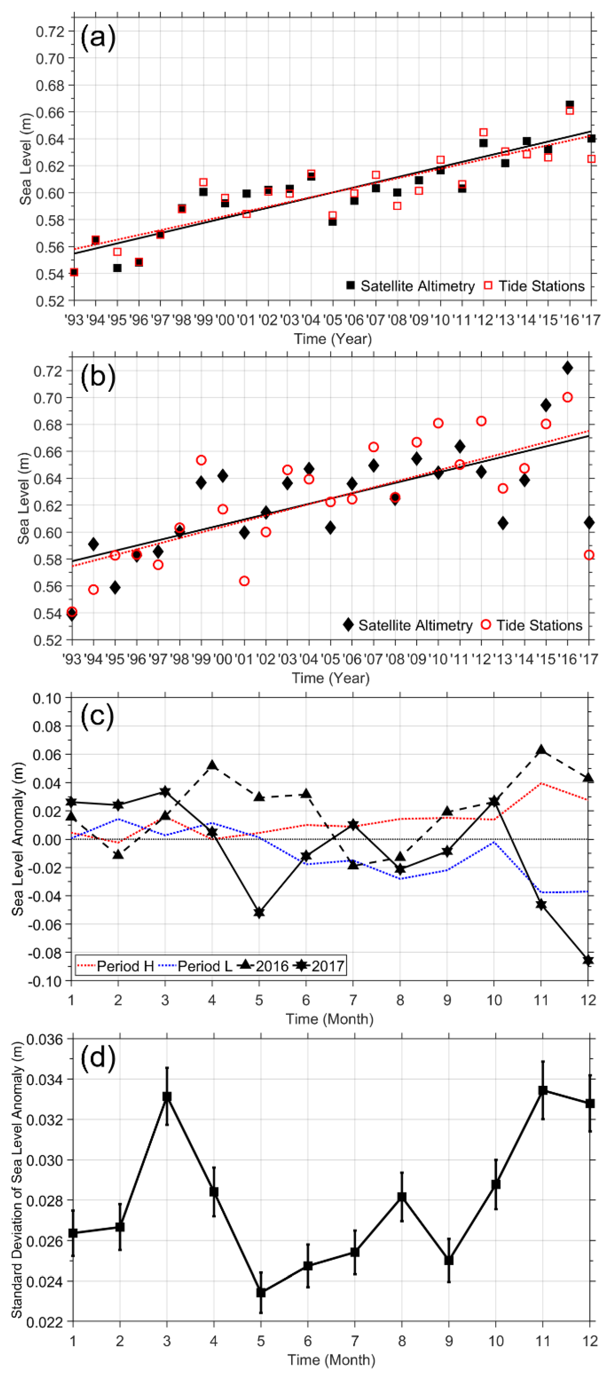
Annual mean sea level observation from satellite altimetry shows a consistent long-term trend and interannual variations in the NEAMS-mean sea level with those obtained from the tide gauge observations indicating a reasonable range of difference. The rate of long-term sea level rise over the period estimated from the ADT of satellite altimetry before being detrended is 3.78 mm   y 1 , which is consistent with those from the tide-gauge observations (3.69 mm   y 1 ). The winter (ND) mean sea level also shows comparable rising rates of satellite altimetry-derived sea level (3.89 mm   y 1 ) and tide-gauge observations (4.41 mm   y 1 ) though the relative magnitude is not consistent, for example, higher rate of annual vs. winter mean sea level rise for tide-gauge vs. satellite observations. A significantly large spread from the linear trend of satellite altimetry-derived annual mean and winter mean sea levels (black lines and symbols in Figure 2a,b) indicates strong interannual variability. For example, the winter mean sea level in the NEAMS, after being detrended, is 0.053 m higher in 2016 and 0.066 m lower in 2017 than the linear trend (corresponding to the black line in Figure 2b and x-axes in Figure 2c and Figure 3); such spreads are particularly large in ND (winter) compared to spreads in other months (Figure 2c,d). High interannual spread of NEAMS-mean sea level in the two months are statistically robust as consistently found from 25 different sets of monthly series of NEAMS-mean sea level for a period of 24 years (excluding one year among the total period of 25 years) with less deviation (vertical bars in Figure 2d). Such noticeable interannual variations of NEAMS-mean sea level in ND (winter), and in March but not in January and February (Figure 2d), motivates us to define and focus on the winter sea level variability.
The annual mean and winter mean sea level anomalies have standard deviations of 0.014 m and 0.028 m (or 1.4 cm and 2.8 cm) and are significantly correlated with each other (correlation coefficient: 0.53, p-value < 0.02), respectively. In contrast to winter (ND), non-winter sea level anomalies derived by averaging sea level over all months except the ND are not significantly correlated with the annual mean sea level (correlation coefficient: 0.21, p-value = 0.30), thereby, highlighting the strong relationship of interannual variability between annual and winter mean sea level anomalies compared to that between annual and non-winter mean sea level anomalies.

3.2. Local Winds During Periods of High vs. Low Sea Levels

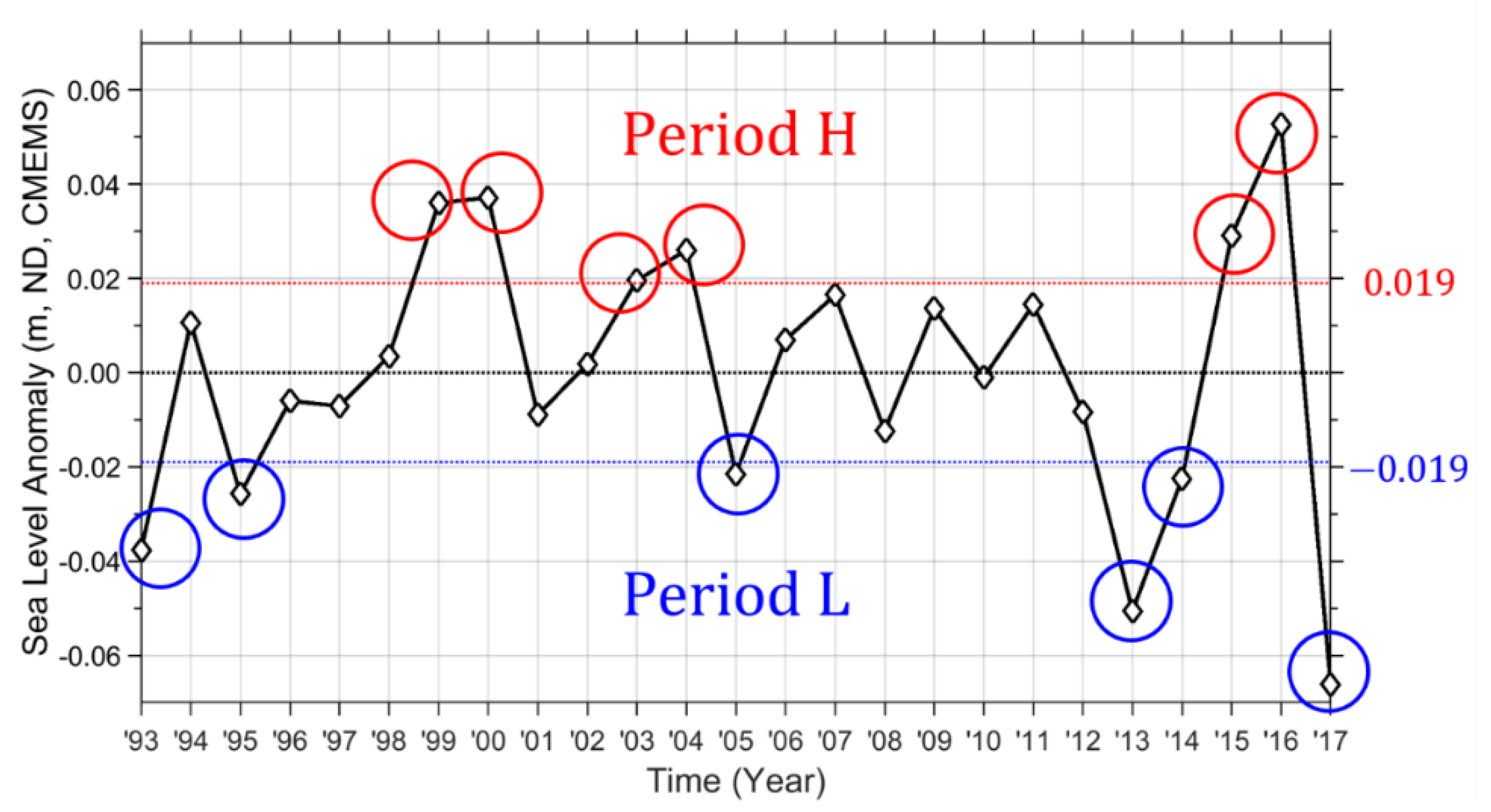
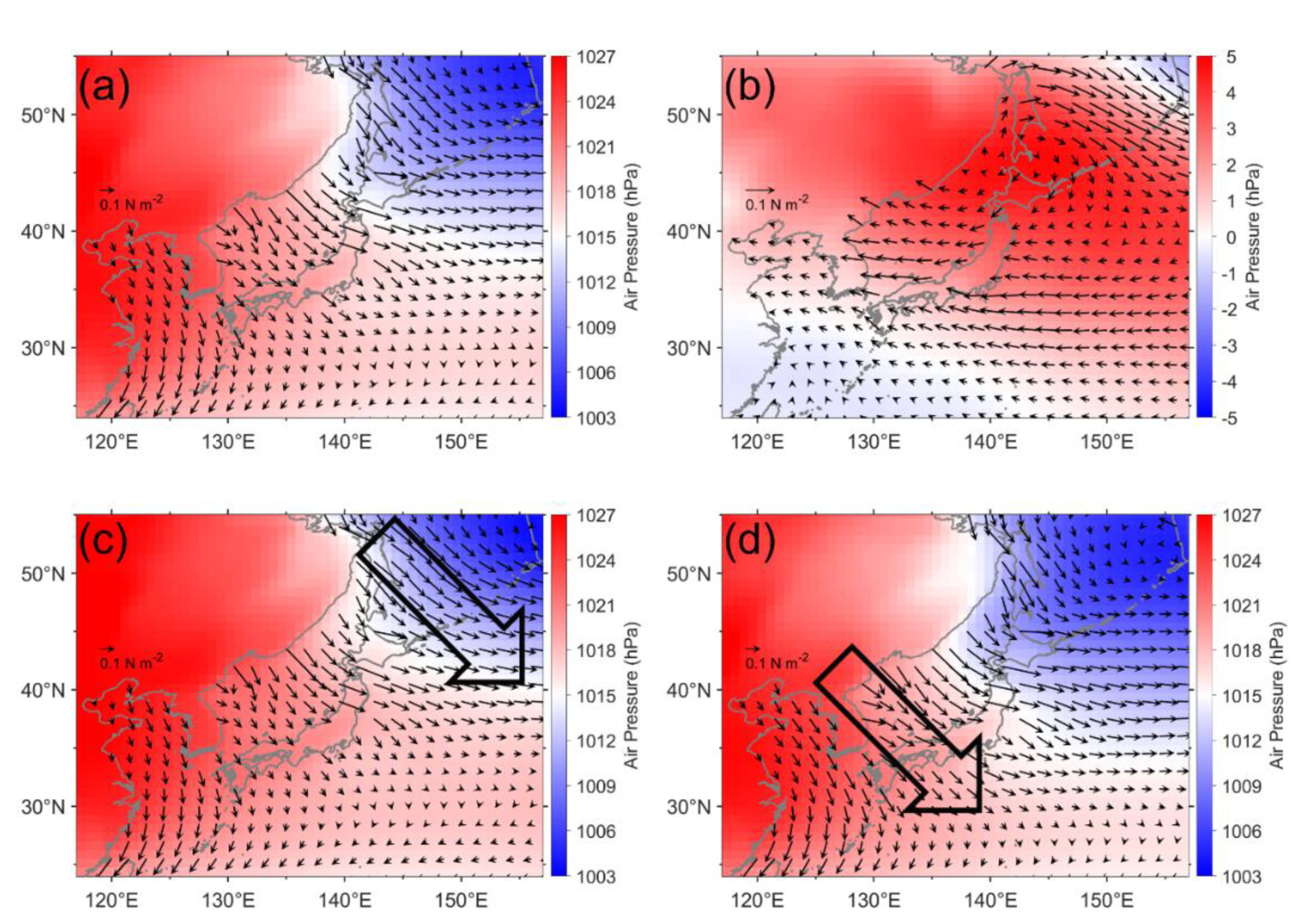
The interannual variations of the winter NEAMS sea level were analyzed to identify six years of relatively high (positive anomalies above +0.019 m) and low (negative anomalies below −0.019 m) sea levels in Period H (1999, 2000, 2003, 2004, 2015, and 2016) and Period L (1993, 1995, 2005, 2013, 2014, and 2017), respectively (Figure 3). Then, the atmospheric pressure fields and associated wind stresses during the two periods were compared to qualitatively account for the high and low winter sea levels in the NEAMS. In the NEAMS, which is influenced by the East Asian winter monsoon, a northwesterly wind prevails in the winter with an enhanced atmospheric pressure gradient between the Siberian High and the Aleutian Low (Figure 4a) as reported in previous studies [24]. During Period H, the Aleutian Low retreats northeastward, and the northwesterly monsoonal wind exerting southeastward wind stress at the sea surface is stronger in the southern SO than in the southern ES (Figure 4c). The Ekman dynamics suggest southwestward Ekman transport within the surface Ekman layer induced by the southeastward wind stress. This causes the obstruction of the outflow transport from the ES to the Pacific (and SO) through the TS and SS resulting in water pile-up or horizontal convergence within the NEAMS (Figure 1 and Figure 4c).
In contrast, during Period L, the Aleutian Low expands southwestward, and a northwesterly monsoonal wind exerting southeastward wind stress at the sea surface is stronger in the southern ES than in the southern SO (Figure 4d). The Ekman dynamics again suggest southwestward Ekman transport within the surface Ekman layer induced by the southeastward wind stress. In this case, the wind-driven Ekman transport would cause the obstruction of the inflow transport from the Pacific to the ECS shelf and from the YECS to the ES through the KS resulting in horizontal divergence within the NEAMS (Figure 1 and Figure 4d). Note that the outflow transport from the ES to the Pacific (and also SO) would not be obstructed in this case because the southeastward wind stress is much weaker in the southern SO during Period L than in Period H (Figure 4d).
Although a northwesterly wind prevails in the SO, ES, and YECS, the atmospheric pressure gradient between the Siberian High and Aleutian Low is noticeable during the winter monsoon. This was previously suggested by [41] and it is confirmed herein based on the mean fields over the total period (Figure 4a). Thus, significant interannual variations in the local atmospheric pressure disturbance and the wind field influence the interannual variability of the winter NEAMS sea level via Ekman dynamics. Westward and southeastward wind stress anomalies in the southern ES and SO, respectively, enhance the inflow transport to the ES and reduce the outflow transport to the Pacific more during Period H than during Period L (Figure 4b).

3.3. Wind-Induced Sea Level Anomalies

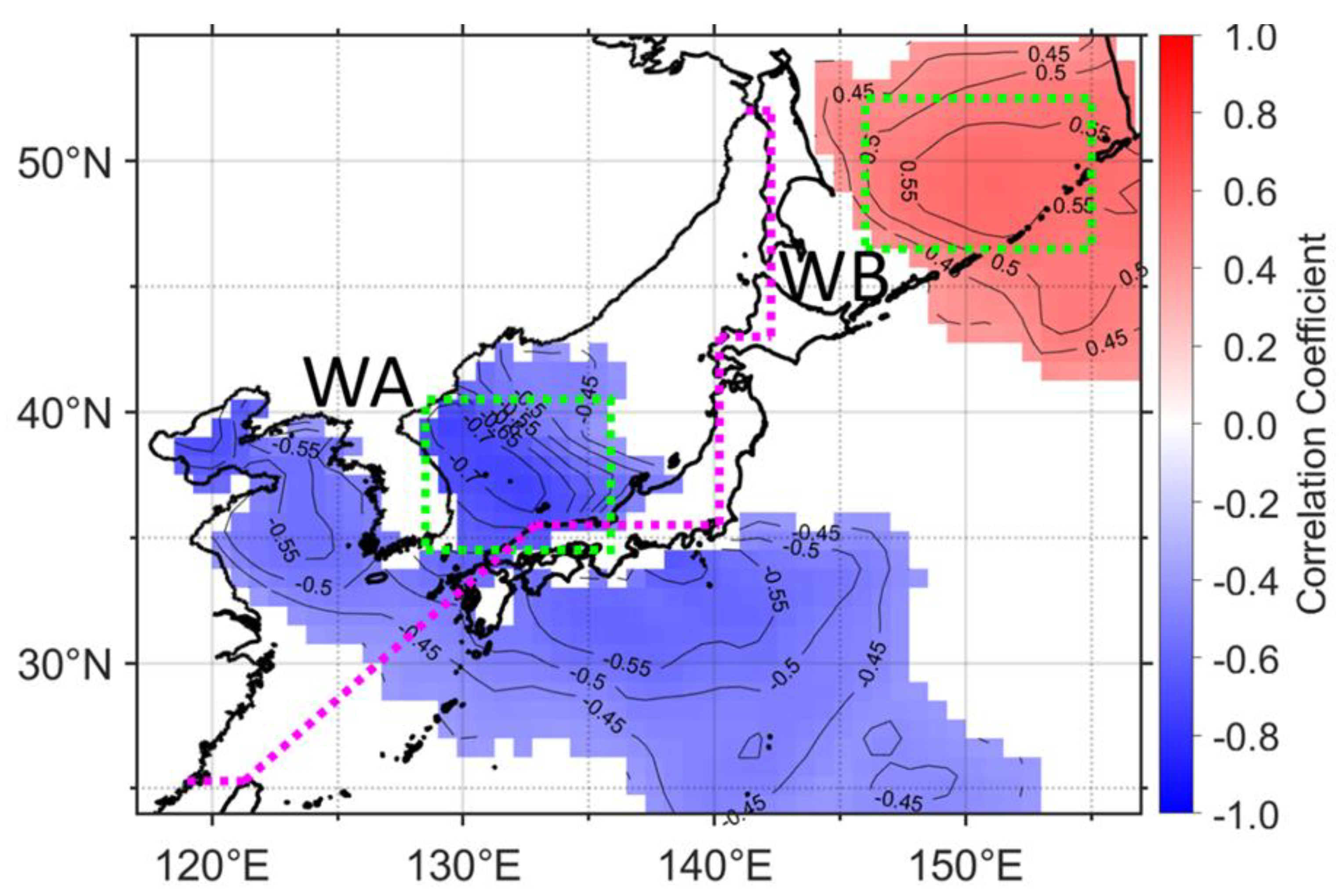
To quantitatively examine the effects of local wind on the winter NEAMS sea level variability, areas of strong interannual southeastward wind stress ( τ S E ) variability that correlate highly with sea level anomalies are identified as WA (128.5–135.9° E, 34.5–40.5° N) and WB (146.0–155.0° E, 46.5–52.5° N) within the ES and SO based on a correlation map between τ S E and sea level anomalies (Figure 5). The correlation map was computed using the 25-year-long time series of NEAMS sea level and those of τ S E at each grid of ECMWF. The correlation map of τ S E with the sea level anomaly indicates positive (negative) values at WB (WA) in the southern SO (ES) demonstrating that high NEAMS sea level occurs with increased (decreased) southeastward wind stress (Figure 5).
The τ S E averaged over the WB (WA) representing local wind forcing in the outflow (inflow) area higher (lower) compared to the 25-year mean by +0.047 N   m 2 (−0.018 N   m 2 ), for example, 0.100 minus 0.053 N   m 2 (0.036 minus 0.054 N   m 2 ) during Period H and lower (higher) by −0.040 N   m 2 (+0.031 N   m 2 ), for example, 0.013 minus 0.053 N   m 2 (0.085 minus 0.054 N   m 2 ) during Period L. Such changes in τ S E can be used to estimate changes in the southwestward Ekman transport per unit length within the surface Ekman layer ( V T E k m a n S W , m 2   s 1 ), as described below:
V T E k m a n S W = D E k m a n 0 u E k m a n S W d z = D E k m a n 0 1 f ρ τ S E z d z =   1 f ρ   { τ S E ( z = 0 ) τ S E ( z = D E k m a n ) }   =   τ S E f ρ .
Here, u E k m a n S W , D E k m a n , f = ( 2 Ω sin φ ) , Ω ≈ (7.2921 × 10 5   rad   s 1 ), φ , ρ , z , and τ S E denote the southwestward Ekman velocity ( m   s 1 ), Ekman depth (m), Coriolis parameter ( rad   s 1 ), rotation rate of the Earth ( rad   s 1 ), latitude, reference density of sea water (≈ 1025 kg   m 3 ), depth (m), and southeastward wind stress ( N   m 2 ), respectively. Then, NEAMS-mean sea level change S L C N E A M S (m) can be estimated as
S L C N E A M S = H C V T N E A M S L T A = ( V T W B V T W A ) L T A
where H C V T N E A M S , V T W A , V T W B , L , T , and A denote horizontal convergence/divergence (positive convergence) of net volume transport into/out of the NEAMS per unit horizontal length scale ( m 2   s 1 ) , horizontal Ekman transports in WA and WB per unit horizontal length scale ( m 2   s 1 ) , horizontal fetch distance scale (m), integration time scale (s), and NEAMS area ( m 2 ), respectively.
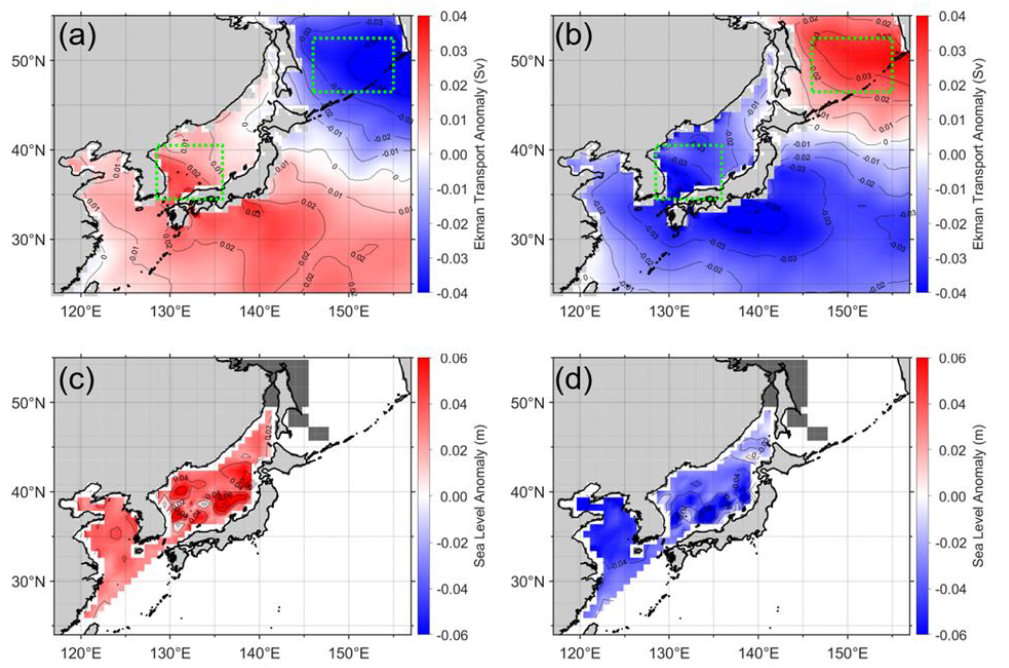
The resulting southwestward Ekman transport anomalies per unit length are +0.408 m 2   s 1 in the WB ( V T W B ) and −0.199 m 2   s 1 in WA ( V T W A ) during Period H (Table 1). They are −0.349 m 2   s 1 in the WB ( V T W B ) and +0.337 m 2   s 1 in WA ( V T W A ) during Period L (Table 1). During Period H, therefore, the horizontal water convergence within NEAMS due to decreased outflow and increased inflow transports reaches 0.607 m 2   s 1 ( H C V T N E A M S ), which corresponds to the order of magnitude (O, 0.01 Sv, 1 Sv = 10 6   m 3   s 1 ) over a horizontal distance of O ( 10 4 m). For example, for a given scale of the horizontal fetch distance of O ( 10 4 m), the volume transport inducing this horizontal convergence across the fetch scale would be 6070 m 3   s 1 (= 0.607 m 2   s 1 × 10 4 m). This volume transport into the NEAMS, integrated over a time scale of one month and divided by the area of the NEAMS, yields a sea level rise of ~1 cm (= 0.0088 m ≈ 0.01 m). Similarly, the horizontal water divergence within the NEAMS due to increased outflow and decreased inflow transports (0.349 m 2   s 1 and 0.337 m 2   s 1 , respectively) is estimated to be 0.686 m 2   s 1 ( H C V T N E A M S ). This corresponds to O (0.01 Sv) over the same horizontal fetch distance of O ( 10 4 m), lowering the NEAMS sea level by O (0.01 m) or ~1 cm in a month in Table 1. Likewise, using Equation (2), the sea level changes induced by wind-driven Ekman transport can be estimated to compare with the NEAMS sea level derived from the satellite altimetry. There is convergence or divergence of wind-driven horizontal transport in the NEAMS (Figure 6a,b) and it can explain the positive or negative NEMAS-mean sea level anomalies (Figure 6c,d).
A multiple linear regression of wind stress anomalies in the WA and WB on the NEAMS sea level anomaly was used to investigate its predictive ability with the following results:
S L A N E A M S = 0.564   τ W A + 0.142   τ W B
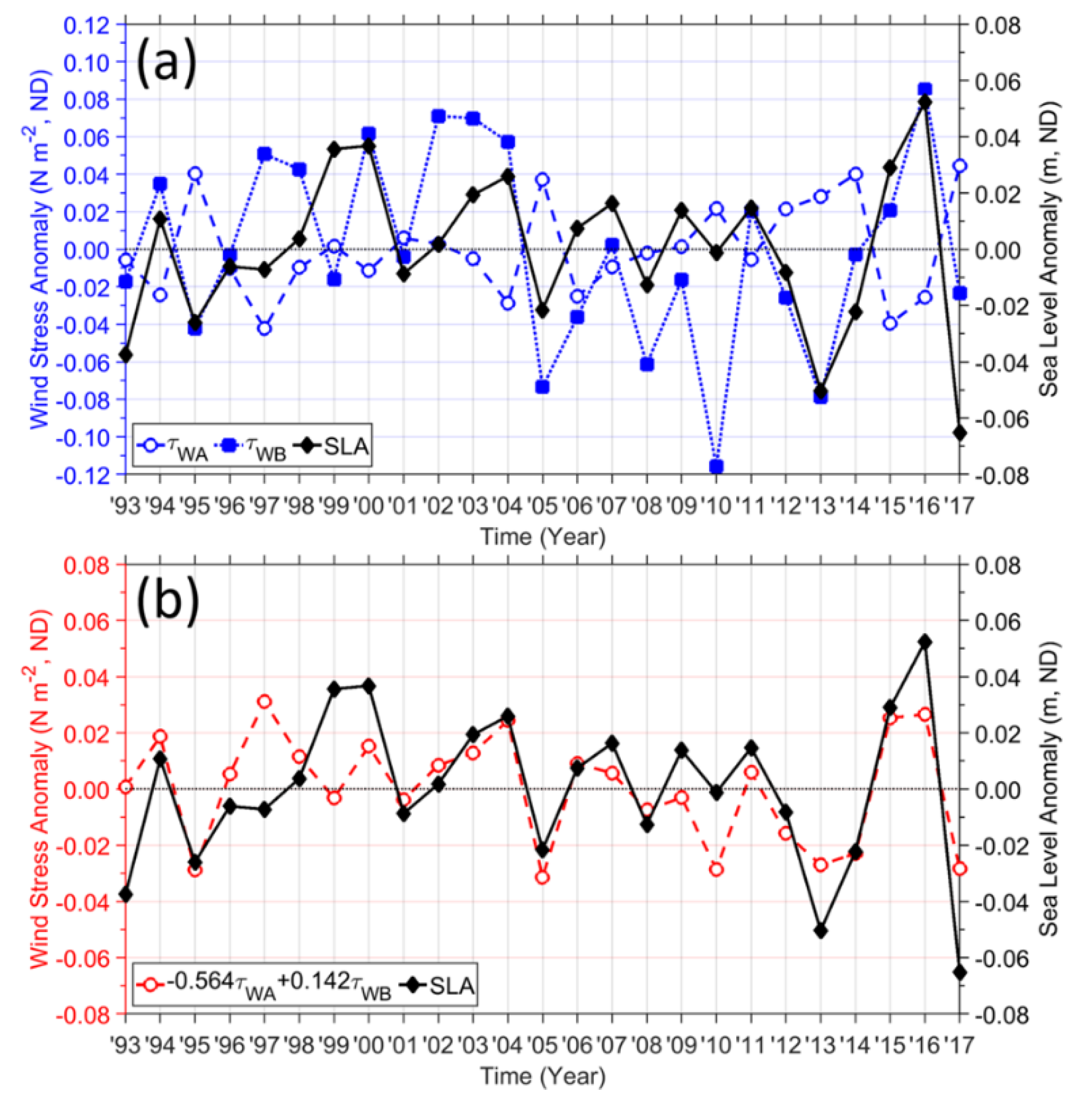
Here, τ W A and τ W B are the southeastward wind stress anomalies averaged over WA and WB, respectively. The results of this multiple linear regression analysis yield a significant correlation coefficient of 0.70 (p-value < 0.01), which is higher than those with τ W A or τ W B (−0.67 and 0.57, respectively), suggesting that the interannual S L A N E A M S variability can be reasonably estimated by τ W A and τ W B (Figure 7). The magnitude of the coefficient of τ W A (0.564) is approximately four times larger than that of τ W B (0.142), and the standard deviation of τ W B is double that of τ W A indicating doubled sensitivity of S L A N E A M S to τ W A compared to τ W B for normalized wind stress anomalies.

3.4. Atmospheric Pressure Disturbances and the Winter NEAMS Sea Level Index (WNSI)

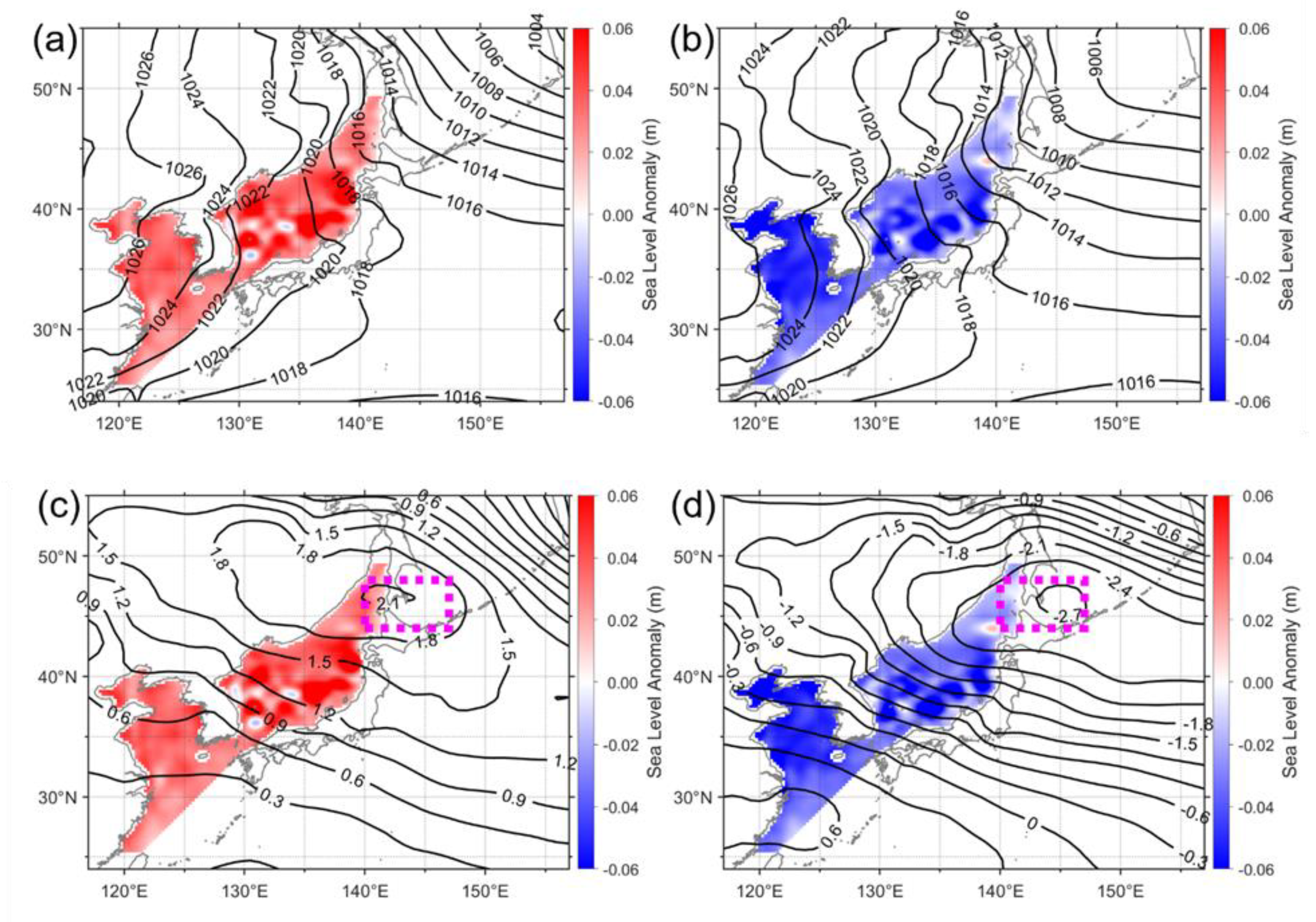
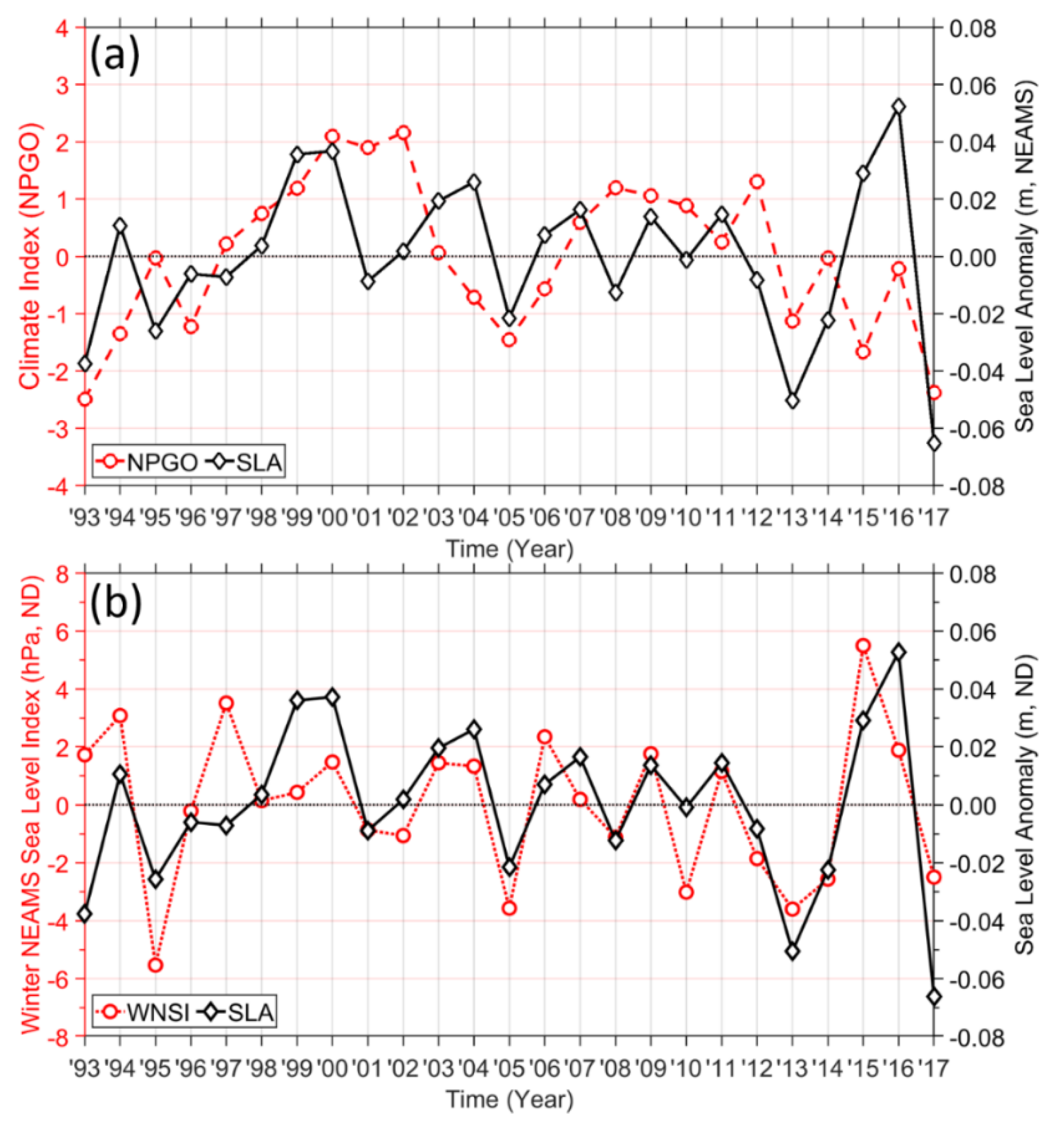
The interannual τ W A and τ W B variations are linked to atmospheric pressure disturbances such as the location of a strong atmospheric pressure gradient between the Siberian High and Aleutian Low (Figure 8). During Period H (Period L), a strong pressure gradient with an enhanced northwesterly wind is located northeast of the SS and in the southern SO (in the vicinity of the KS and the southern ES) (Figure 8a,b), yielding higher (lower) than normal atmospheric pressures around the SS (e.g., magenta dotted box in Figure 8c,d). The enhanced northwesterly wind or southeastward wind stress anomaly in the southern SO corresponds to horizontal convergence in the NEAMS and positive winter NEAMS-mean sea level anomaly. Thus, a new index called the winter NEAMS sea level index (WNSI) is defined herein as the atmospheric pressure anomaly in hPa averaged over the area around the SS (140.0–147.0° E, 44.0–48.0° N), where the local atmospheric pressure anomalies reach their maximum (Period H) and minimum (Period L) values. The reason for choosing atmospheric pressure anomalies in the area rather than spatial atmospheric pressure difference is that it is dynamically linked to the relative strength between northwesterly monsoonal winds in the southern ES and SO. The WNSI is significantly correlated with S L A N E A M S (correlation coefficient: 0.62, p-value < 0.01) (Figure 9b), demonstrating a similar predictability to that of wind stress anomalies ( τ W A and τ W B ) or a better predictability than that of other climate indices that represent remote forcing. These climate indices are the Pacific Decadal Oscillation (PDO), North Pacific Gyre Oscillation (NPGO), North Pacific Index (NPI), Oceanic Niño Index (ONI), Arctic Oscillation Index (AOI), East Asian Winter Monsoon Index (EAWMI), Siberian High Index (SHI), and Aleutian Low-Pressure Index (ALPI), and their correlations with S L A N E A M S are insignificant except for that of the NPGO (Figure 9a). The correlation coefficients of annual mean and winter (ND) mean indices are listed in Table 2. The correlation coefficient of the multiple linear regression results of winter NPGO and WNSI with the winter NEAMS-mean sea level anomaly is 0.78 (p-value < 0.01) indicating marginally (though not markedly) improved predictive skills by including the remote effect.

4. Discussion

The results of the interannual variability of the winter NEAMS sea level induced by local wind stress forcing linked to atmospheric pressure disturbances presented in this study are consistent with the results of previous studies in several aspects. The surface wind stress has been suggested as one of the most important contributors to sea level changes in marginal seas [22,23,24], and sea level changes induced by zonal wind stresses linked to meridional migration of the sub-polar front in the ES have been reported previously [26]. Basin-scale oscillations of the ES mean sea level forced by high-frequency (a few days to a few weeks) atmospheric pressure forcing and constrained by narrow and shallow straits (KS, TS, and SS) in relation to rapidly propagating barotropic waves have also been previously reported [5,16,21]. For low-frequency (e.g., periods longer than 100 days) forcing, the sea level change outside the ES constrains water exchange across the straits implying that the ES basin-scale oscillations can be extended outside the ES. This study confirms this possibility, revealing basin-scale oscillations across the NEAMS with the inclusion of a shallow YECS. The rapidly propagating barotropic waves homogenize the sea level across the NEAMS as well as the ES, particularly for low-frequency (including interannual) timescales. Note that significant roles of wind forcing on changing sea level in the ECS have also been reported previously [22,23,24,42,43].
Although this study demonstrates the critical role of the southeastward wind stress in the changing winter NEAMS sea level via horizontal water convergence and divergence, the thermosteric and halosteric effects of the properties of sea water transported into/out of the NEAMS on the sea level variability have not been considered. As the water carried by the inflow transport to the NEAMS across the ECS shelf and the KS is warmer and more saline than that carried by the outflow transport from the NEAMS across the TS and SS, the increased inflow transport would increase sea level more than the decreased outflow transport would for the same volume of convergence. Future studies need to address the thermosteric and halosteric effects of sea water properties along with wind-driven Ekman transport.
A better estimation of interannual winter NEAMS-mean sea level variability is obtained by using the local atmospheric pressure anomaly (WNSI, Figure 9b) or by multiple linear regressions of the local wind stress anomalies in WA and WB (Figure 7) rather than from the estimates made using climate indices (remote forcing) including the NPGO (Figure 9a). The local atmospheric pressure disturbance that is proxied well by the Ekman transport associated with wind stress anomalies is maximized in the area around the SS (magenta dotted box in Figure 8c,d). This reflects the importance of local wind-driven horizontal transport (Ekman transport) into or out of the NEAMS on low-frequency (interannual) sea level oscillations in lieu of atmospheric pressure loading in contrast to the critical role of non-isostatic sea level responses to atmospheric pressure in the ES for high-frequency sea level oscillations [5,7,16,21]. However, this does not mean that the winter NEAMS-mean sea level is always more affected by the local atmospheric forcing than remote forcing or entirely irrelevant to the large-scale pattern of variability in the open Pacific Ocean. In particular, the winter NEAMS-mean sea level is significantly correlated with the NPGO and multiple linear regression of WNSI and NPGO considering both local and remote forcing marginally better account for the interannual sea level variability than the case of WNSI only. Neither WNSI nor multiple linear regression of wind stress anomalies representing the local forcing agree well with the winter NEAMS-mean sea levels from 1997 to 1999, when conventional or eastern Pacific-type El Niño (1997–1998) and La Niña (1998–2000) events occurred, implying certain roles of remote forcing via atmospheric teleconnections in changing the NEAMS sea level during those years potentially relevant to decadal oscillations linked to the NPGO (Figure 7 and Figure 9). This is particularly true considering the footprint of the El Niño Southern Oscillation or regime shift on the YECS during a couple of (but not all) decades [44,45], thereby, suggesting the use of multiple linear regression analyses of local atmospheric pressure anomalies (WNSI) and climate indices (NPGO) for achieving better prediction.
Although the wind-induced Ekman transports within the semi-enclosed deep and shallow basins in the NEAMS play a key role in the interannual variability of winter mean sea level, another mechanism for this variability can be considered. A cooling process due to the 18% increase in sea surface wind speed (5.37 m   s 1 compared to 4.57 m   s 1 ) via increased heat loss from the NEAMS into the atmosphere may lower the thermosteric sea level during Period L compared to Period H. Using the winter mean turbulent (sensible plus latent) heat flux of ~300 W   m 2 reported for the region [46], 13% higher and 5% lower cooling effects are estimated due to sea surface wind speeds (5.37 m   s 1 compared to 4.82 m   s 1 and 4.57 m   s 1 compared to 4.82 m   s 1 , respectively), which are stronger during Period L and weaker during Period H compared to the mean for the total period. The resultant turbulent heat fluxes are 285 W   m 2 (= 300–(300 × 0.05)) during Period H and 339 W   m 2 (= 300 + (300 × 0.13)) during Period L. However, sea surface cooling corresponding to the stronger wind speed lowers the steric sea level by only O ( 10 3 m), which can be estimated based on the thermal expansion coefficient of 1.48 × 10 4 ° C 1 and density of 1025 kg m 3 corresponding to climatological mean temperature and salinity at the upper 250 m averaged over the NEAMS from 1995 to 2017 using Equation (4) below:
S L D C o o l i n g = ( | u A i r L | | u A i r H | 1 ) · α · T · T H F ρ C p .
Here,   S L D C o o l i n g , | u A i r H | , | u A i r L | , α , T H F , and C p denote sea level decreased by cooling due to the 18% increase in wind speed in Period L than in Period H (m), wind speeds ( m   s 1 ) during Periods H and L, respectively, thermal expansion coefficient ( ° C 1 ), amount of turbulent heat loss, and specific heat capacity ( J   kg 1   ° C 1 ) , respectively. Then, the scale of winter NEAMS-mean sea level lowered by enhanced cooling during Period L compared to that of Period H is −0.0051 m or −0.51 cm , which is one order of magnitude smaller than those induced by the anomalous Ekman transports O ( 10 2 m), in other words, ( 0.18 )   ×   ( 1.48   ×   10 4   ° C 1 )   ×   (   60   ( s )   ×   60   ( m )   ×   24   ( hr )   ×   30.5   ( d )   )   ×   ( 300   W   m 2 ) / { ( 1025   kg   m 3 )   ×   ( 3993   J   kg 1   ° C 1 ) } . The anomalous heat loss via ~54 W   m 2 (= 339–285   W   m 2 ) represents more turbulent heat flux corresponding to a positive anomaly in wind speed that may cool the surface water more in the region and yielding a sea level drop of ~0.0051 m at the most, in other words, less than 1 cm. Freshwater exchange between the atmosphere and ocean can affect the halosteric sea level, but it is even smaller by a factor of 10 than that of the thermosteric sea level in the region [12]. Therefore, we rule this possibility out as well from being the key mechanism for the interannual variability of winter NEAMS-mean sea level.

5. Conclusions

We presented the interannual variations of winter sea levels averaged over the NEAMS for a 25-year period from 1993 to 2017, which were successfully explained by horizontal water convergence and divergence due to monsoonal wind-induced Ekman transport. Composite analyses with two contrasting periods of high (Period H) and low (Period L) NEAMS sea level anomalies and correlation analyses with spatial patterns of southeastward wind anomalies and atmospheric pressure differences between the two marginal seas, ES and SO, around the SS were conducted. The results reveal that the winter NEAMS sea level rises (drops) with water convergence (divergence) with stronger southeastward wind stress in the southern SO (ES) than in the southern ES (SO) during Period H (Period L) (Figure 10). The Ekman dynamics suggest that the stronger southeastward wind stress in the southern SO induces decreased outflow transport from the ES to the Pacific Ocean and SO through the TS and SS. Furthermore, increased wind-driven inflow transport from the Pacific Ocean to the YECS via the shelf intrusion and to the ES through the KS along with the decreased outflow transport play a key role in raising the winter NEAMS-mean sea level during Period H. Our results highlight the important roles of local wind forcing and Ekman dynamics in changing the winter sea level variability in the NEAMS, thereby providing a better predictability with atmospheric pressure anomalies proxied via WNSI (correlation coefficient: 0.62 with p-value < 0.01), multiple regressions of wind stress anomalies, or both WNSI and NPGO together rather than by remote forcing only (climate indices).

Author Contributions

Conceptualization, M.H., S.N., and Y.-K.C.; methodology, M.H., S.N., Y.-K.C., and H.-W.K.; formal analysis, M.H.; investigation, M.H., S.N., Y.-K.C., and H.-W.K.; writing—original draft preparation, M.H.; writing—review and editing, M.H. and S.N.; visualization, M.H.; supervision, S.N. and Y.-K.C.; project administration, K.-Y.J. and E.L. All authors have read and agreed to the published version of the manuscript.

Funding

This work was funded by the Korea Hydrographic and Oceanographic Agency (KHOA) through the “Analysis and Prediction of Sea Level Change in Response to Climate Change around the Korean Peninsula” program. This research was a part of the project titled “Deep Water Circulation and Material Cycling in the East Sea (20160040)” and “Construction of Ocean Research Stations and their Applications in Studies”, funded by the Ministry of Oceans and Fisheries, Republic of Korea. H.-W.K. is supported by KIOST in-house project (PE99811).

Acknowledgments

We would like to thank the five reviewers for their constructive comments and suggestions, and Editage (http://www.editage.co.kr) for English language editing. Satellite altimetry data (SSALTO/DUACS altimeter products) produced and distributed by the CMEMS (http://www.marine.copernicus.eu), tide-gauge sea level data provided by the Permanent Service for Mean Sea Level (PSMSL; http://www.psmsl.org/data/obtaining), and surface air-pressure and wind stress data from the ECMWF interim reanalysis (http://www.ecmwf.int/) were used in this study.

Conflicts of Interest

The authors declare no conflict of interest.

References

  1. Mangiarotti, S.; Lyard, F. Surface pressure and wind stress effects on sea level change estimations from TOPEX/Poseidon satellite altimetry in the Mediterranean Sea. J. Atmos. Ocean. Technol. 2008, 25, 464–474. [Google Scholar] [CrossRef]
  2. Pinardi, N.; Bonaduce, A.; Navarra, A.; Dobricic, S.; Oddo, P. The mean sea level equation and its application to the Mediterranean Sea. J. Clim. 2014, 27, 442–447. [Google Scholar] [CrossRef]
  3. Park, K.-A.; Lee, E.-Y.; Chang, E.; Hong, S. Spatial and temporal variability of sea surface temperature and warming trends in the Yellow Sea. J. Mar. Syst. 2015, 143, 24–38. [Google Scholar] [CrossRef]
  4. Zhang, Z.-M.; Yang, G.-P.; Zhang, H.-H.; Shi, X.-Z.; Zou, Y.-W.; Zhang, J. Phthalic acid esters in the sea-surface microlayer, seawater and sediments of the East China Sea: Spatiotemporal variation and ecological risk assessment. Environ. Pollut. 2020, 259, 113802. [Google Scholar] [CrossRef] [PubMed]
  5. Lyu, S.J.; Kim, K.; Perkins, H.T. Atmospheric pressure-forced subinertial variations in the transport through the Korea Strait. Geophys. Res. Lett. 2002, 29, 1–8. [Google Scholar] [CrossRef]
  6. Park, J.-H.; Watts, D.R.; Wimbush, M.; Book, J.W.; Tracey, K.L.; Xu, Y. Rapid Variability in the Japan/East Sea: Basin Oscillations, Internal Tides, and Near-inertial Oscillations. Oceanography 2006, 19, 76–85. [Google Scholar] [CrossRef] [Green Version]
  7. Nam, S.; Park, J.-H.; Park, J.J. High-frequency variability: Basin-scale oscillations and internal waves/tides. In Oceanography of the East Sea (Japan Sea); Springer: Berlin/Heidelberg, Germany, 2016; pp. 127–148. [Google Scholar] [CrossRef]
  8. Gordon, A.L.; Giulivi, C.F. Pacific decadal oscillation and sea level in the Japan/East Sea. Deep Sea Res. Part I Oceanogr. Res. Pap. 2004, 51, 653–663. [Google Scholar] [CrossRef]
  9. Moon, J.-H.; Lee, J. Shifts in multi-decadal sea level trends in the East/Japan Sea over the past 60 years. Ocean Sci. J. 2016, 51, 87–96. [Google Scholar] [CrossRef]
  10. Moon, J.-H.; Song, Y.T. Decadal sea level variability in the East China Sea linked to the North Pacific Gyre Oscillation. Cont. Shelf Res. 2017, 143, 278–285. [Google Scholar] [CrossRef]
  11. Yasuda, T.; Sakurai, K. Interdecadal variability of the sea surface height around Japan. Geophys. Res. Lett. 2006, 33. [Google Scholar] [CrossRef]
  12. Kang, S.K.; Cherniawsky, J.Y.; Foreman, M.G.G.; Min, H.S.; Kim, C.; Kang, H. Patterns of recent sea level rise in the East/Japan Sea from satellite altimetry and in situ data. J. Geophys. Res. Oceans 2005, 110. [Google Scholar] [CrossRef]
  13. Kang, S.K.; Cherniawsky, J.Y.; Foreman, M.G.G.; So, J.; Lee, S.R. Spatial variability in annual sea level variations around the Korean peninsula. Geophys. Res. Lett. 2008, 35. [Google Scholar] [CrossRef]
  14. Kim, C.-H.; Jang, C.J.; Kim, M.-W. A Numerical Simulation of Long-Term Sea Level Change in the East Asian Marginal Seas. J. Coast. Res. 2018, 85, 546–550. [Google Scholar] [CrossRef]
  15. Choi, B.; Haidvogel, D.B.; Cho, Y. Nonseasonal sea level variations in the Japan/East Sea from satellite altimeter data. J. Geophys. Res. Oceans 2004, 109. [Google Scholar] [CrossRef] [Green Version]
  16. Nam, S.H.; Lyu, S.J.; Kim, Y.H.; Kim, K.; Park, J.; Watts, D.R. Correction of TOPEX/POSEIDON altimeter data for nonisostatic sea level response to atmospheric pressure in the Japan/East Sea. Geophys. Res. Lett. 2004, 31. [Google Scholar] [CrossRef] [Green Version]
  17. Choi, B.-J.; Cho, S.H.; Jung, H.S.; Lee, S.-H.; Byun, D.-S.; Kwon, K. Interannual variation of surface circulation in the Japan/East Sea due to external forcings and intrinsic variability. Ocean Sci. J. 2018, 53, 1–16. [Google Scholar] [CrossRef]
  18. Jacobs, G.A.; Teague, W.J.; Riedlinger, S.K.; Preller, R.H.; Blaha, J.P. Sea surface height variations in the Yellow and East China Seas: 2. SSH variability in the weekly and semiweekly bands. J. Geophys. Res. Oceans 1998, 103, 18479–18496. [Google Scholar] [CrossRef]
  19. Wang, G.; Kang, J.; Yan, G.; Han, G.; Han, Q. Spatio-temporal variability of sea level in the East China Sea. J. Coast. Res. 2015, 73, 40–47. [Google Scholar] [CrossRef]
  20. Hirose, N.; Ostrovskii, A.G. Quasi-biennial variability in the Japan Sea. J. Geophys. Res. Oceans 2000, 105, 14011–14027. [Google Scholar] [CrossRef]
  21. Lyu, S.J.; Kim, K. Subinertial to interannual transport variations in the Korea Strait and their possible mechanisms. J. Geophys. Res. Oceans 2005, 110. [Google Scholar] [CrossRef]
  22. Zuo, J.; He, Q.; Chen, C.; Chen, M.; Xu, Q. Sea level variability in East China Sea and its response to ENSO. Water Sci. Eng. 2012, 5, 164–174. [Google Scholar]
  23. Zhang, S.; Du, L.; Wang, H.; Jiang, H. Regional sea level variation on interannual timescale in the East China Sea. Int. J. Geosci. 2014, 5, 1405. [Google Scholar] [CrossRef] [Green Version]
  24. Yu, K.; Liu, H.; Chen, Y.; Dong, C.; Dong, J.; Yan, Y.; Wang, D. Impacts of the mid-latitude westerlies anomaly on the decadal sea level variability east of China. Clim. Dyn. 2019, 53, 5985–5998. [Google Scholar] [CrossRef]
  25. Ohshima, K.I.; Simizu, D.; Ebuchi, N.; Morishima, S.; Kashiwase, H. Volume, heat, and salt transports through the Soya Strait and their seasonal and interannual variations. J. Phys. Oceanogr. 2017, 47, 999–1019. [Google Scholar] [CrossRef]
  26. Choi, B.-J.; Haidvogel, D.B.; Cho, Y.-K. Interannual variation of the Polar Front in the Japan/East Sea from summertime hydrography and sea level data. J. Mar. Syst. 2009, 78, 351–362. [Google Scholar] [CrossRef]
  27. Han, M.; Cho, Y.-K.; Kang, H.-W.; Nam, S.; Byun, D.-S.; Jeong, K.-Y.; Lee, E. Impacts of Atmospheric Pressure on the Annual Maximum of Monthly Sea-Levels in the Northeast Asian Marginal Seas. J. Mar. Sci. Eng. 2020, 8, 425. [Google Scholar] [CrossRef]
  28. CMEMS. Global Ocean Gridded L4 Sea Surface Heights and Derived Variables Reprocessed (1993–Ongoing). Available online: http://marine.copernicus.eu/services-portfolio/access-to-products/?option=com_csw&view=details&product_id=SEALEVEL_GLO_PHY_L4_REP_OBSERVATIONS_008_047 (accessed on 6 March 2020).
  29. Pujol, M.; Schaeffer, P.; Faugère, Y.; Raynal, M.; Dibarboure, G.; Picot, N. Gauging the improvement of recent mean sea surface models: A new approach for identifying and quantifying their errors. J. Geophys. Res. Oceans 2018, 123, 5889–5911. [Google Scholar] [CrossRef]
  30. Fecher, T.; Pail, R.; Gruber, T.; Consortium, G. GOCO05c: A new combined gravity field model based on full normal equations and regionally varying weighting. Surv. Geophys. 2017, 38, 571–590. [Google Scholar] [CrossRef]
  31. Mayer-Guerr, T. The combined satellite gravity field model GOCO05s. EGUGA 2015, 2015, 12364. [Google Scholar]
  32. Park, Y.; Park, T.; Kim, T.; Lee, S.; Hong, C.; Lee, J.; Rio, M.; Pujol, M.; Ballarotta, M.; Durand, I. Observations of the Antarctic Circumpolar Current over the Udintsev Fracture Zone, the narrowest choke point in the Southern Ocean. J. Geophys. Res. Oceans 2019, 124, 4511–4528. [Google Scholar] [CrossRef] [Green Version]
  33. Marcos, M.; Tsimplis, M.N.; Calafat, F.M. Inter-annual and decadal sea level variations in the northwestern Pacific marginal seas. Prog. Oceanogr. 2012, 105, 4–21. [Google Scholar] [CrossRef]
  34. Morimoto, A. Evaluation of tidal error in altimetry data in the Asian marginal seas. J. Oceanogr. 2009, 65, 477–485. [Google Scholar] [CrossRef]
  35. Holgate, S.J.; Matthews, A.; Woodworth, P.L.; Rickards, L.J.; Tamisiea, M.E.; Bradshaw, E.; Foden, P.R.; Gordon, K.M.; Jevrejeva, S.; Pugh, J. New data systems and products at the permanent service for mean sea level. J. Coast. Res. 2013, 29, 493–504. [Google Scholar]
  36. PSMSL. Permanent Service for Mean Sea Level Tide Gauge Data. Available online: http://www.psmsl.org/data/obtaining/ (accessed on 9 September 2019).
  37. Mathers, E.L.; Woodworth, P.L. Departures from the local inverse barometer model observed in altimeter and tide gauge data and in a global barotropic numerical model. J. Geophys. Res. Oceans 2001, 106, 6957–6972. [Google Scholar] [CrossRef]
  38. Wen, C.; Kumar, A.; Xue, Y. Uncertainties in reanalysis surface wind stress and their relationship with observing systems. Clim. Dyn. 2019, 52, 3061–3307. [Google Scholar] [CrossRef]
  39. WOA. World Ocean Atlas 2018 (WOA18). Available online: https://www.nodc.noaa.gov/OC5/woa18/woa18data.html (accessed on 15 June 2020).
  40. Price, J.F.; Weller, R.A.; Schudlich, R.R. Wind-driven ocean currents and Ekman transport. Science 1987, 238, 1534–1538. [Google Scholar] [CrossRef] [Green Version]
  41. Jhun, J.-G.; Lee, E.-J. A new East Asian winter monsoon index and associated characteristics of the winter monsoon. J. Clim. 2004, 17, 711–726. [Google Scholar] [CrossRef]
  42. Liu, X.; Liu, Y.; Guo, L.; Rong, Z.; Gu, Y.; Liu, Y. Interannual changes of sea level in the two regions of East China Sea and different responses to ENSO. Glob. Planet. Chang. 2010, 72, 215–226. [Google Scholar] [CrossRef]
  43. Li, Y.; Zuo, J.; Lu, Q.; Zhang, H.; Chen, M. Impacts of wind forcing on sea level variations in the East China Sea: Local and remote effects. J. Mar. Syst. 2016, 154, 172–180. [Google Scholar] [CrossRef]
  44. Thompson, B.; Tkalich, P.; Malanotte-Rizzoli, P. Regime shift of the South China Sea SST in the late 1990s. Clim. Dyn. 2017, 48, 1873–1882. [Google Scholar] [CrossRef] [Green Version]
  45. Kim, Y.S.; Jang, C.J.; Yeh, S.-W. Recent surface cooling in the Yellow and East China Seas and the associated North Pacific climate regime shift. Cont. Shelf Res. 2018, 156, 43–54. [Google Scholar] [CrossRef]
  46. Yeo, D.-E.; Nam, S. Seasonal and spatial variations of air-sea heat exchange in the seas around the Korean Peninsula: Based on the observations and reanalysis products from 2011 to 2016. Prog. Oceanogr. 2020, 181, 102239. [Google Scholar] [CrossRef]
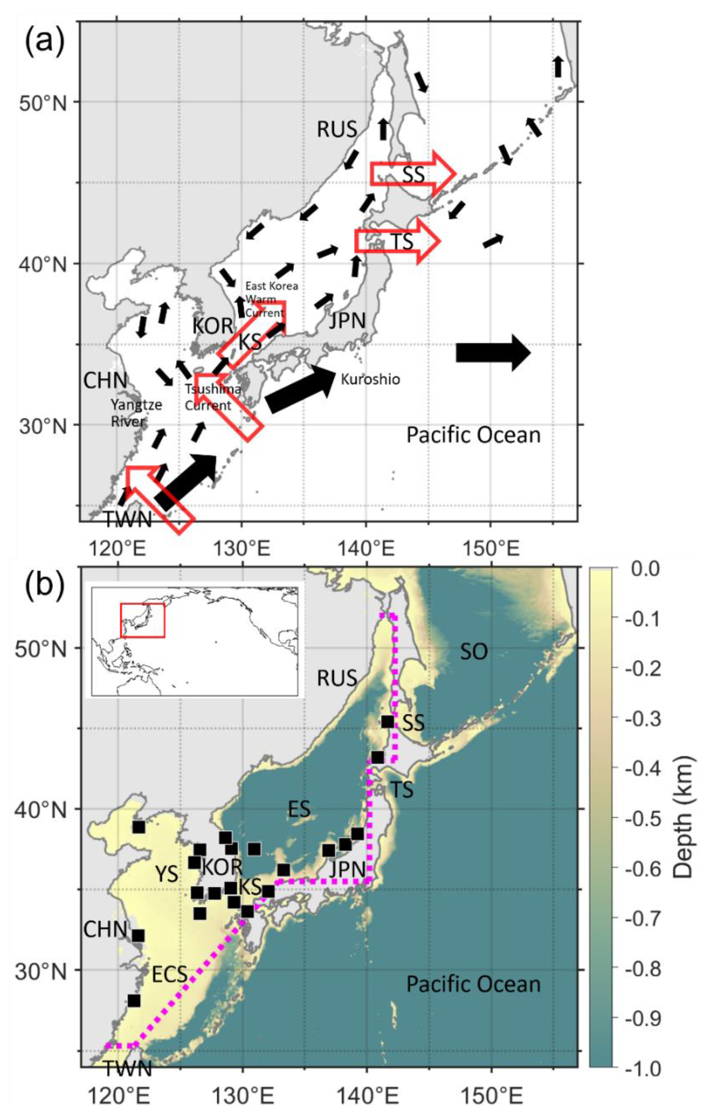
Figure 1. (a) Schematics of the regional circulation patterns with major surfaces currents in the northeast Asian marginal seas (NEAMS). The stronger Kuroshio is shown with thicker arrows while other currents are indicated by black filled arrows, respectively. Red open arrows represent major inflow and outflow volume transports. (b) Domain (area indicated with magenta dotted lines) and location (red box in the world map in the upper left corner) of the NEAMS, local bathymetry (colors), and locations of tide gauge stations selected for this study (black squares, available at https://www.psmsl.org). KOR, RUS, CHN, TWN, and JPN are the abbreviations for Korea, Russia, China, Taiwan, and Japan, respectively. YS, ECS, ES, and SO indicate the Yellow Sea, East China Sea, East Sea (Sea of Japan), and Sea of Okhotsk, respectively. KS, TS, and SS represent the Korea/Tsushima Strait, Tsugaru Strait, and Soya Strait, respectively.
Jmse 08 00774 g001
Figure 2. Time series of (a) annual mean and (b) winter (ND) mean NEAMS sea levels estimated from satellite altimetry (black squares and diamonds) and tide-gauge observations (red open squares and circles) from 1993 to 2017, (c) detrended monthly mean NEAMS sea levels in Period H (red dotted line), Period L (blue dotted line), 2016 (dashed line with black triangles), and 2017 (solid line with black hexagrams), and (d) monthly series of an interannual spread of the climatological mean NEAMS sea levels derived from mean (squares) and standard deviation (vertical bars) of 25 different subsamples of monthly series for a period of 24 years among the total period of 25 years from 1993 to 2017.
Jmse 08 00774 g002
Figure 3. Time series of the detrended winter (ND) mean sea-level anomalies averaged over the NEAMS from 1993 to 2017, in which six years of high (above +0.019 m) or low (below −0.019 m) winter sea level anomalies are indicated as Period H (1999, 2000, 2003, 2004, 2015, and 2016) or Period L (1993, 1995, 2005, 2013, 2014, and 2017) with red and blue circles, respectively.
Jmse 08 00774 g003
Figure 4. Composite maps of mean atmospheric pressure at sea level (hPa, colors) and wind stress ( N   m 2 , small arrows) in winter (a) for the total period of 25 years (1993–2017) and (b) their differences between Periods H and L (Period H shown in (c) minus Period L shown in (d)). Composite maps of mean atmospheric pressure at sea level (hPa, colors), surface wind stress ( N   m 2 , small arrows), and strong northwesterly monsoonal winds exerting southeastward wind stress on the sea surface (large open arrows) in winter for (c) Period H and (d) Period L.
Jmse 08 00774 g004
Figure 5. Correlation map of the NEAMS winter sea level with the surface wind stress anomaly in the southeast (+)–northwest (−) direction from 1993 to 2017. The contour interval is 0.05 and correlations with less than 95% significances were discarded. A positive correlation means that a high (low) NEAMS sea level occurs with a strong southeastward (northwestward) wind stress anomaly. Here, the areas showing the maximum positive (WB) and negative (WA) correlation coefficients are marked with green dotted boxes and the NEAMS is indicated with magenta dotted lines.
Jmse 08 00774 g005
Figure 6. The horizontal Ekman transport anomaly in Sv during (a) Period H and (b) Period L. Positive sign means eastward and northward Ekman transport anomaly. The areas of WA and WB are marked with green dotted boxes. The sea level anomaly distribution within the NEAMS area derived from satellite altimetry observations during (c) Period H and (d) Period L. Light and dark grey colors indicate land and ice areas, respectively.
Jmse 08 00774 g006
Figure 7. Time series of (a) southeastward wind stress anomalies in the WA (blue dashed line, left y-axis) and WB (blue dotted line, left y-axis), (b) multiple linear regression results from southeastward wind stress anomalies in the WA and WB on the NEAMS-mean sea level anomalies (red dashed line, left y-axis), and (a,b) winter NEAMS-mean sea level anomaly observed from satellite altimetry (black line, right y-axis) from 1993 to 2017. The correlation coefficients of the NEAMS-mean sea level anomalies with wind stress anomalies in the WA and WB are −0.67 (p-value < 0.01) and 0.57 (p-value < 0.01) while that with multiple linear regression is 0.70 (p-value < 0.01).
Jmse 08 00774 g007
Figure 8. (a,b) Winter atmospheric pressure field at sea level (black contours) and (c,d) atmospheric pressure anomalies (black contours) during (a,c) Period H and (b,d) Period L. Here, winter NEAMS sea level anomalies are superimposed using a color scale (red: positive, blue: negative), and the area defining the NEAMS sea-level index is indicated with magenta dotted boxes (c,d).
Jmse 08 00774 g008
Figure 9. Time series of winter NEAMS-mean sea level anomalies (black line) and (a) the North Pacific Gyre Oscillation (NPGO) index (red dashed line) and (b) winter NEAMS-mean sea level index based on local atmospheric pressure anomaly (WNSI, red dotted line) from 1993 to 2017. Correlation coefficients are (a) 0.41 with p-value = 0.04 and (b) 0.62 with p-value < 0.01, respectively.
Jmse 08 00774 g009
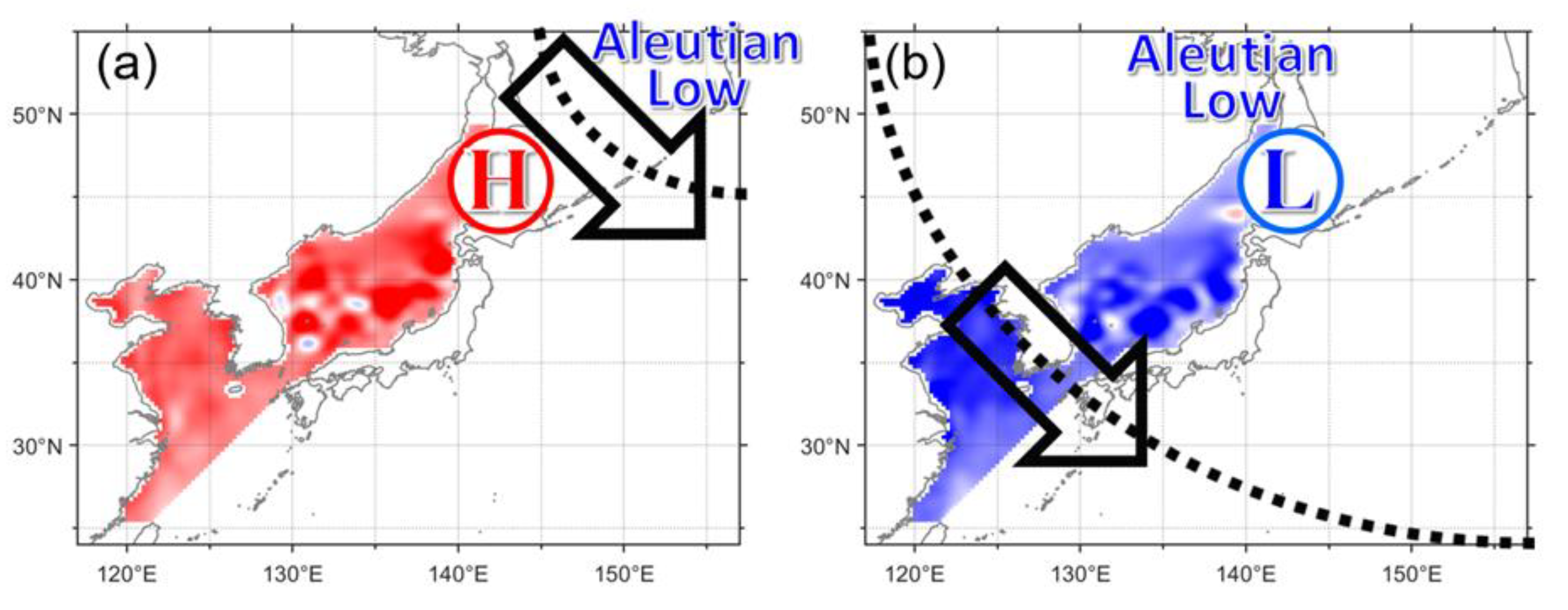
Figure 10. Schematic diagrams accounting for the winter NEAMS sea level anomalies. (a) A stronger winter monsoon with northwesterly wind or southeastward wind stress (black arrows) and associated atmospheric pressure gradients (black dotted lines) in the southern SO; e.g., the northeastward retreat of the Aleutian Low obstructs the outflow transport from the ES into the Pacific by Ekman dynamics to yield a higher (red) NEAMS sea level during Period H. (b) In contrast, a stronger winter monsoon in the southern ES obstructs the inflow transport from the Pacific to the ECS shelf and to the ES to yield a lower (blue) NEAMS sea level during Period L.
Jmse 08 00774 g010
Table 1. Scaling estimation for southwestward Ekman transport per unit horizontal length scale within the surface Ekman layer ( V T E k m a n S W ) , horizontal convergence/divergence due to net volume transport into/out of the NEAMS per unit horizontal length scale ( H C V T N E A M S ), and NEAMS-mean sea level change ( S L C N E A M S ) in Periods H and L.
RegionPeriod HPeriod L
V T E k m a n S W ( m 2   s 1 )WA τ S E W A f ρ = 0.018 0.89 × 10 4 × 1025   = 0.199 τ S E W A f ρ = + 0.031 0.89 × 10 4 × 1025   = + 0.337
WB τ S E W B f ρ = + 0.047 1.12 × 10 4 × 1025   = + 0.408 τ S E W B f ρ = 0.040 1.12 × 10 4 × 1025   = 0.349
H C V T N E A M S ( m 2   s 1 )NEAMS V T W B V T W A = τ S E W B f ρ τ S E W A f ρ = 0.408 + 0.199 = 0.607 V T W B V T W A = τ S E W B f ρ τ S E W A f ρ = 0.349 0.337 = 0.686
S L C N E A M S (m)NEAMS ( V T O u t V T I n ) L T A = 0.607 × 10 4 × 2.6 × 10 6   1.8 × 10 12   = 0.0088 ( V T O u t V T I n ) L T A = 0.686 × 10 4 × 2.6 × 10 6   1.8 × 10 12   = 0.0099
Table 2. Correlation coefficients (and p-values) of annual mean and winter (ND) mean climate indices with the winter NEAMS-mean sea level anomaly. Values significant at the 95% confidence level are in bold.
Climate IndexAnnual MeanWinter Mean
PDO−0.09 (0.66)−0.16 (0.45)
NPGO+0.49 (0.01)+0.41 (0.04)
NPI−0.15 (0.49)−0.05 (0.80)
ONI+0.24 (0.25)+0.09 (0.66)
AOI−0.03 (0.87)+0.10 (0.63)
EAWMI−0.32 (0.12)−0.23 (0.26)
SHI−0.08 (0.69)−0.16 (0.44)
ALPI+0.09 (0.69)Not available