Abstract
To estimate the response of wave energy converters to different sea environments accurately is an ongoing challenge for researchers and industry, considering that there has to be a balance between guaranteeing their integrity whilst extracting the wave energy efficiently. For oscillating wave surge converters, the incident wave field is changed due to the pitching motion of the flap structure. A key component influencing this motion response is the Power Take-Off system used. Based on OpenFOAM, this paper includes the Power Take-off to establish a realistic model to simulate the operation of a three-dimensional oscillating wave surge converter by solving Reynolds Averaged Navier-Stokes equations. It examines the relationship between incident waves and the perturbed fluid field near the flap, which is of great importance when performing in arrays as neighbouring devices may influence each other. Furthermore, it investigates the influence of different control strategy systems (active and passive) in the energy extracted from regular waves related to the performance of the device. This system is estimated for each wave frequency considered and the results show the efficiency of the energy extracted from the waves is related to high amplitude pitching motions of the device in short periods of time.
1. Introduction
The Oscillating Wave Surge Converter (OWSC) is one of the most promising operating devices that use Wave Energy Conversion (WEC) technology in terms of its energy absorption capabilities and hydrodynamic performance [1]. This device consists of a surface-piercing buoyant flap rotating around a hinge fixed to the sea bottom. The pitching motion of the WEC device combined with a hydraulic Power Take-Off (PTO), which connects the flap to its base, captures the energy from nearshore ocean surface waves [2].
The OWSC operates usually at intermediate water depth where the energy is extracted from the surge motion of the waves [3]. Under the action of these incident waves, the flap oscillates back and forth (see Figure 1). This oscillatory motion is dominated by the diffraction and the radiation effects of the incident wave acting on the device. Whilst the first is related to the solid body as an obstacle encountered by the fluid flow, the latter is identified with the oscillatory motion of the flap and consequent generation of secondary wave fields. Both effects will depend on the size of the flap and its oscillation [4].
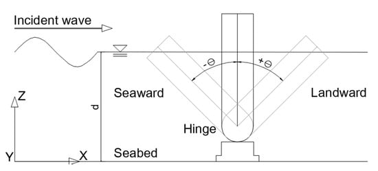
Figure 1.
Schematic drawing showing the motion of an oscillating wave surge converter induced by incident waves.
In conjunction with the Queen’s University Belfast (QUB), Aquamarine Power (AP) developed and deployed the full-scale prototype of an OWSC called Oyster at the EMEC (European Marine Energy Centre) site in Orkney. During and after the designing stage of the Oyster, QUB in cooperation with AP undertook extensive experimental and numerical studies. These studies focused mainly on understanding the hydrodynamic response of the OWSC in different wave environments as well as in increasing its performance.
Initial experimental studies regarding the response of a flap-type surface-piercing WEC to waves are reported in [5,6]. These were early estimations of the power output and performance of the energy device under the action of small amplitude regular waves. Further two-dimensional experimental studies for OWSC were undertaken in order to understand the wave slamming phenomenon when the device operates in extreme sea conditions [7,8].
Using experimental models to understand the hydrodynamic performance of OWSC is generally demanding in terms of cost and time. To complement these experimental tests, numerical models are a viable alternative to estimate the performance of wave energy converters in the early stages of design. Various approaches of numerical modelling have been implemented to understand the hydrodynamic performance of OWSC with incident wave fields. These approaches include using the method based on the potential flow theory [9,10], the smoothed particle hydrodynamics (SPH) method [11,12], and the Computational Fluid Dynamics (CFD) method based on the Navier-Stokes equations.
Among these methods, the CFD approach has been widely used in hydrodynamic problems, as it can capture more realistic phenomena than linear theoretical approaches, whilst is much more convenient than experiments [13,14,15,16]. Studies of the hydrodynamic response of OWSC to ocean waves have been carried out in [6,17,18] using the CFD approach. For the dynamic motion of the flap under the effect of the incident waves, these numerical models have used body-fitted mesh for small angular displacements and arbitrary coupled mesh interface (ACMI) for large motions. In [19], the two-dimensional model of an OWSC performing under extreme sea conditions was studied using OpenFOAM software to solve the Reynolds-Averaged Navier-Stokes (RANS) equations combined with the overset mesh approach to handle the dynamic motion for large amplitudes.
One of the first sub-systems to be included when modelling wave energy converters is the Power Take-Off (PTO), since this is one of the main elements influencing the power capture assessment in the performance of the device [20]. The PTO is used to transform the mechanical energy of the moving flap into electrical energy; for the OWSC device, this can be done using a hydraulic system, electro-mechanical, or permanent-magnet reciprocating generators [21,22].
Nonetheless, to represent the PTO accurately when performing experimental and numerical simulations is a continuous challenge due to the complex systems associated with the control strategy of the PTO [12,21]. Previous work considering the influence of the PTO in the operation of the OWSC includes the experimental work done by [23,24] and the numerical and semi-analytical studies undertaken by [24,25,26,27,28]. In these semi-analytical studies, the fluid problem set up using linear theory is solved by the application of numerical methods. To assess the power performance of WEC with the nonlinear PTO system, a high-fidelity CFD solution can be used [20].
For numerical simulations, these systems can be modelled as reactive/active or resistive/passive controls by simplifying the force models adding external forces/moments back to WEC system, represented as spring-damper or damper systems, respectively. In reactive control strategies, the spring and damper coefficients are adjusted to achieve the maximum power absorption for each wave frequency, specifically by tuning the stiffness to the natural frequency of the WEC device [29,30]. In this condition, the damping coefficient of the PTO is considered as the radiation damping coefficient of the device. Whereas for resistive controls, the stiffness coefficient is set to zero and the damping coefficient is optimised. The PTO has been represented as a rotational linear spring-damper or damper systems for surface-piercing OWSC numerically in [12,28,31].
For most of WEC devices, the efficiency is maximized when its frequency is tuned with the frequency of the wave, i.e., performing in resonance. Nonetheless, for the Oyster, this is not necessary since its operating principle depends on the exciting torque acting on the flap [10], which was further investigated in [31]. In this study, different cases considering underdamped, overdamped, and damped models were analysed. Within these results, it was shown that the relation of the optimum damping is not linearly dependent on the wave frequency.
In [12], an OWSC combined with a PTO was studied by SPH and validated against experimental tests. Moreover, the influence of the PTO damping characteristics and flap inertia in the power capture of the device was investigated. The range of the regular wave conditions of the 1:10 model includes wave heights between 0.15 and 0.25 m and a wave period of 2.0 s (corresponding to a wavelength of 4.90 m). Furthermore, it was proved that the PTO system should not be neglected when analysing the hydrodynamics of OWSC for its influence on the Capture Width Ratio (CWR) of the device. The wave field, specifically the free surface elevation and the velocity distributions, is affected according to the damping coefficients used.
Further numerical studies solving RANS equations including WEC devices considering different control strategies have been validated against experimental studies in [32,33]. Whilst in [32], the device considered is the Wavestar, in [33] is a set of Point Absorbers performing in different array configurations.
As a general appraisal, finding conditions for the device to operate as efficiently as possible at a constant rate is a challenge. To measure the efficiency of the power capture of a single unit, the Capture Width Ratio (CWR) is employed. This non-dimensional quantity relates the Capture Width, defined as the ratio of the total mean power absorbed by the WEC to the mean power per unit wave width of the incident wave, to the characteristic length of the device. It can also be quantified by using the Maximum Capture Width Ratio (MCWR), where the PTO mechanism is optimised for a specific wave frequency [34].
The objective of this study is to understand the influence in the wave energy extraction of the OWSC of different control strategies using the RANS method. Whilst the second aim is to use these results to analyse the wave pattern field around the WEC device operating under different wave conditions. In order to attain these goals, an undamped OWSC (as shown in Figure 1) is validated using OpenFOAM against experimental results. Following, the optimal damping coefficient, Bopt, at each wave frequency is calculated using the hydrodynamic coefficients for a flap-type pitching WEC in [28]. For the spring-damper system, the pitching stiffness coefficient, K, is taken for a vertical parallelepiped flap with uniform distributed mass. For each wave condition considered, the power capture factor, that is, the percentage of energy available in the wave train absorbed by the damper and spring-damper PTO, is calculated. Further, the resulting wave field pattern around the device is analysed.
Following this introduction, this paper presents the employed numerical theories, the development of the CFD model, and the validations of the model against OWSC experiments. Particularly, a practical approach to account for the PTO is introduced and the influence of the PTO on the power capture is investigated. The wave field around a single OWSC device is simulated and analysed, considering the condition where the power capture factor was higher for a spring-damper control strategy. Finally, the conclusion includes a brief summary and the implications of this study, as well as recommendations for further studies.
2. Numerical Approach
Linear wave theory has been successfully used to understand the hydrodynamic forces acting on surface piercing Oscillating Wave Surge Converters (OWSC) when performing in isolation under normal operating conditions. For this condition, the wave height is small compared to the wavelength and to the dimension of the body. Nevertheless, for Power Take-Off (PTO) implications in the power capture and when operating under rough sea conditions, this theory is no longer applicable due to the presence of additional non-linear effects. The use of fully nonlinear viscous models, such as the Reynolds Averaged Navier-Stokes (RANS) approach combined with Volume of Fluid (VoF) method to handle the free surface, has previously been shown to be satisfactory to understand the hydrodynamic behaviour of OWSC devices performing in adverse sea conditions [6,17,35].
For the wave–structure interaction problem using overset grid approach, the RANS equations are first solved throughout the domain to estimate the fluid velocity and pressure distribution. Following that, to obtain the hydrodynamic force acting on the body located within the overset grid, the fluid pressure is integrated over the body’s surface. Once the forces and moments acting on the body have been calculated, the translational and angular momentum equations of the rigid body are solved for its motion. Finally, the fluid and body properties and the overset mesh are updated, and the simulation continues with the iteration for the next time step. The motion of the body is handled by building a dynamic mesh around the flap.
2.1. Fluid Solution
The numerical model used for this study was first validated using a two-dimensional model in previous work [19]. In this current work, it was extended to be three-dimensional with a PTO system implemented. The simulation of the Numerical Wave Tank (NWT) with the flap-type WEC device is developed using the open-source software OpenFOAM. In the tank, two immiscible incompressible fluids, water and air, are considered. The governing equations for this multiphase system include the continuity and momentum equations presented below:
U and g are the velocity and gravity vector fields, respectively. The density is and p* is the pseudo-dynamic pressure, p = ρg∙x (used as a numerical technique for the solution), x is the position vector and is the dynamic viscosity. To close the equations for the solution of the RANS equations, the k-ω (Shear Stress Tensor, SST) turbulence model is used, which has been successfully used for wave-structure interaction for high pressure gradients and flow separation [6].
To handle the motion of the free surface, the Volume of Fluid (VoF) method, introduced in [36], is used. In this approach, a volume fraction constant, , is used to identify the quantity of liquid in each cell of the numerical domain. If is equal to 1 the cell is filled with water, whereas if it is 0, the cell is filled with air. In the case where has a value between 0 and 1, that cell has part water and part air, and therefore, these cells contain the free surface.
Field values such as the velocity U, the density , and the dynamic viscosity of the cell are calculated using the weighted average field value of each fluid as follows:
where is a general representation of the field to be replaced to form each field variable equation.
The variation of the volume fraction is done using the advection equation. This equation tracks the fluid interface movement and is solved simultaneously with Equations (1) and (2):
To estimate the pressure and velocity fields across the multiphase system, the Finite Volume Method (FVM) is used. This numerical approach solves the governing Partial Differential Equations (PDEs) by transforming them into a discrete algebraic equation system over control volumes. These control volumes, or cells, fill the computational domain completely and are connected through their interfaces. In the case of a structured mesh, such as the one used for this study, the use of FVM is convenient, since the interpolation of the fluxes from the cell centres to the faces is more precise. More information about this method can be found in [37,38,39,40].
For the velocity-pressure coupling solution, the PIMPLE algorithm is used; this is a mixture of the PISO (Pressure Implicit with Splitting of Operators) and SIMPLE (Semi-Implicit Method for Pressure-Linked Equations) solving procedures, as explained in [37,38]. The main structure of PIMPLE is based on the PISO solver, but the stability of the solution is improved; less iterations are required for the solution and the simulation speed is incremented.
The solution of the governing equations by using the FVM is achieved through space and time equation discretisation. The discretisation of the mesh of the background domain is constructed with hexahedral cells, whilst the motion of the flap-type device is handled using the overset mesh, which is further explained below. As for the time discretisation, the time-step is adjusted using the Courant Number (CFL). This number relates to the velocity flux crossing a grid cell in a given time-step. By using adjustable time discretisation, the time-step used is fixed according to the estimated value of the velocity in the cell, the size of the cell, and the limit of CFL.
The static boundary method combined with active wave absorption as detailed in [41] is used for the generation of linear regular waves and absorption for the NWT. The pressure is calculated within the numerical model whilst the values of the velocity fields and the free surface elevation are corrected in the wave generation patch according to the wave theory applied. The free surface is measured at the patch at each time step and compared to the theoretical value, and corrected accordingly by modifying the U and α boundary conditions. The static boundary wave generator is combined with active wave absorption, and by thus, dissipation zones are not needed, and unnecessary water level increase is avoided. The methodology is further detailed in [41,42]. The most common wave conditions for power production are considered in the present study; therefore, highly nonlinear waves related to extreme conditions are not considered. Moreover, in this study, regular waves based on the operation site of the full-scale prototype, found in [43], are used.
2.2. Body Motion
Throughout this work the OWSC device is assumed to be a rigid body with one degree of freedom (DOF), which is the pitching motion around the y-axis. In Figure 2a, the regions of the overset meshes are shown in a 2D-schematic model, in which the background mesh considers the generation of the waves and the multiphase flow, whilst the front mesh handles the motion of the rigid body and the multiphase flow in its surroundings. The data are interpolated between these two meshes and the volume occupied by the rigid body is cut from the background and front domains and the body surface will move along with the fluid field.
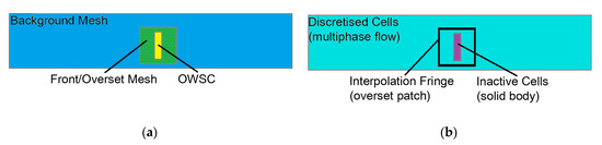
Figure 2.
(a) Overlapping meshes. (1) Background mesh: Consists of the two-phase flow of the Numerical Wave Tank (NWT), (2) overset or front mesh: Consists of the surrounding mesh of the solid body, and, (3) Oscillating Wave Surge Converter (OWSC): The body is conformed using the Cartesian cell cut technique; (b) control volumes. (1) Discretisation cells: Discretise the governing equations of the multiphase flow, (2) interpolation cells: The solution is interpolated from mesh to mesh, and (3) inactive cells: No solution is done.
To apply this approach, the control volumes are identified as inactive, interpolation, and discretisation cells (see Figure 2b). The solution for the inactive cells is not computed, as they simulate the rigid body, the interpolation cells contains the solution interpolated from mesh to mesh at every time-step, and the discretisation cells is where the discretisation of the governing equations of the multiphase flow is solved. In this region, the fringe cells (located at the outer boundary of the overset mesh) are the interpolation cells connected to donor stencils from the background mesh. The method for the overset interpolation is the inverse distance instead of the cell volume weight method, since the former have proved to be less time consuming than the latter for three-dimensional cases [44]. In this study, the cell sizes of the overset or front mesh are changed to match the size of the background mesh size, as this will minimise the interpolation error when the background and front meshes are communicating [44,45].
The total force and moments come from the fluid and wave loads acting on the flap, the damping force exerted by the oscillatory motion of the flap, and the restraint acting at the hinge at the bottom of the device. The fluid forces, F, considered are the surface forces (pressure, normal, and shear stresses), , as well as the body forces (gravitational forces), . The surface forces are calculated at each time-step of the numerical simulation by integrating the pressure and the viscous stress components over the wetted surface of the rigid body, SB, whilst the body forces include the gravitational force, as follows:
where p is the pressure, I is the unit or identity tensor of size (3 × 3), τ is the viscous stress tensor, n is the unit normal vector to the body surface, m is the mass of the rigid body, g is the acceleration of the gravity vector, and SB is the wetted surface.
Similarly, the total moment of the OWSC device, M, is calculated at each time-step as the sum of all the components acting around the hinge:
where r is the position vector (x, y, z), is the position of the centre of gravity at a time-step, and is the hinge position. For the power capture calculations, an additional external moment is applied to the hinge, as will be introduced in Section 3.2.
The motion equation for the rigid body is based on the linear and angular momentum equations:
where and are the linear and angular accelerations, respectively, and is the moment of inertia of the rigid body.
To obtain the velocity and displacement of the rigid body the Newmark time integration scheme, introduced in [46], is applied during the numerical simulation. The angular velocities and the displacements of the body are obtained from the following equations [47]:
where is the angular velocity vector of the body, is the angular displacement vector of the body, is the velocity integration coefficient, is the position integration coefficient, is the time-step, super script “t” is used for the values obtained on the previous iteration, whilst “t + ” is for the values at the current time being simulated. The recommended values for is 0.5, whilst for is 0.25 [48], which are the ones used in this simulation.
3. Results and Discussion
3.1. Verification and Validation
The setup for the validation of the CFD model is based on the experimental test undertaken in QUB with a 1:40 scale model, whose particulars are retrieved from [6]. For the numerical tank, the dimensions considered are 20.0 × 1.8 × 0.6 m (length × width × height), and, the water depth is 0.34 m. In the case of the flap-type energy converter model, its dimensions are 0.10 × 0.65 × 0.34 m (thickness × width × height) and it rotates around the hinge located at 0.12 m from the bottom of the NWT (see the schematic model in Figure 3). The distance from the bottom of the plate simulating the OWSC to the bottom of the NWT is 0.10 m; this space corresponds to that occupied by the fixed base of the device. The mass of the flap is 10.77 kg, and its mass moment of inertia is 0.1750 kg-m2 whilst the centre of gravity is at 0.12 m measured from the hinge. The flap-type model is located at 12.2 m from the wave-maker and waves generated are with height of 0.038 m and period of 2.063 s, with its wavelength corresponding to 4.2 m.
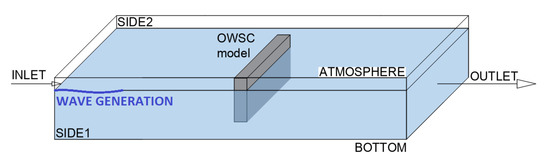
Figure 3.
Schematic of the numerical model, including the tank and the wave energy device.
Before including the device within the NWT, the wave generated was validated against theoretical values. Furthermore, an initial mesh sensitivity test for the wave generation is undertaken. For this spatial discretisation different cell sizes were considered; in Table 1, the number of cells per wavelength (CPW) and the number of cells per wave height (CPH) for the different mesh sizes considered are shown. The wave surface elevation was measured at 12.2 m, where the device would be located, and compared to the theoretical results of a sinusoidal wave (Stokes first order); the average of the relative error calculated for the crests and troughs are presented also in Table 1. For this case, after case “St1_V4” the results already converge and there are no significant changes in the values measured. This means that considering 140 CPW and 19 CPH gives a good accuracy for the generated wave at the inlet.

Table 1.
Cell sizes considered in the mesh sensitivity study for the generated wave of height 0.038 m and period 2.063 s.
The results of the free surface elevation measured during the experimental tests are published in [6] and retrieved from a period between 8 and 12 s to be compared to the results of the converged case “St1_V4” in Figure 4. It is worth noting that the experimental measurement was done at 1 m from the centre line of the tank (and of the OWSC) to its side. Whilst the troughs seem to match, there is a difference on the difference in the crests of the waves. During the experimental tests this difference was related to reflected or radiated waves in [6]. For this validation study, this approximated wave (first order Stokes’ wave theory) was used.
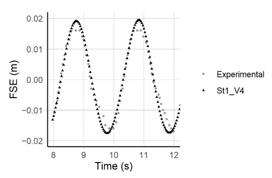
Figure 4.
Free Surface Elevation (FSE) measured at 12.2 m of the inlet of the wave tank.
For the analysis of the domain discretisation, the numerical simulations have been done considering three refined meshes by the use of a refinement ratio of approximately √2 as recommended in [49,50], to the x- and z- directions. Due to the geometry constraints/accuracy required when cutting the holes for the rigid body modelling, the exact refinement ratio of √2 could not be met, hence it is within a range of 1.5–2.0, depending on the case (see Table 2). The refined meshes considered have 120, 180, and 240 CPW and 8, 16, and 30 CPH, respectively. In each case, the overset mesh (R3) was matched to the size of the background mesh. The width of the tank was discretised using cells of 0.05 m size (the same for the overset mesh in that direction). The NWT has been refined in the areas of interest, namely the region close to the flap-type device and the free surface, R1 and R2, respectively, as seen in Figure 5.
Table 2.
Root Mean Squared Error (RMSE) calculated using the results of the rotation angles.
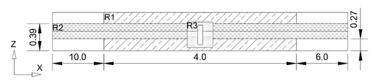
Figure 5.
Mesh refined regions in the model (Units: Meters. Measures are not in scale. R1: Region close to the device, R2: Free surface region, and R3: Overset/front mesh).
The numerical results obtained of the rotation angles and angular velocity of the device performing under linear waves are presented against an oscillation period in Figure 6. In both graphs, the results obtained using 120 CPW are lower to those obtained with the refined cases. These last two cases seem to have reached the convergence, since between them, there is no notable difference between the rotation and angular velocity values. In Table 2, the values of the Root Mean-Squared Error (RMSE) calculated for the rotation angles are presented, where the error is decreased for the medium and refined meshes, CPW 180 and CPW 240, respectively, which shows a monotonic convergence has been achieved.
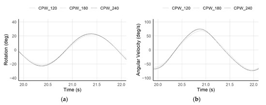
Figure 6.
Influence of varying mesh density in the: (a) Rotation angle, (b) angular velocity.
The experimental test results of the 1:40 scale OWSC model, done at QUB [6], were used for the validation of the numerical model. These results included the tangential and radial accelerations, and these are compared to the numerical results undertaken in this study, as presented in Figure 7.
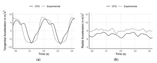
Figure 7.
Tangential (a) and radial (b) accelerations of the numerical (Computational Fluid Dynamics (CFD)) and experimental values measured at the OWSC.
The tangential acceleration is obtained by the equation , where is the tangential acceleration (m/s2), is the angular acceleration (rad/s2), and is the radius measured from the hinge location to the top of the plate. The equation for the radial acceleration is , where is the angular velocity (rad/s). However, for validation purposes, and in order to compare with the experimental tests is obtained from the equation , where is the total acceleration of the body in (m/s2) obtained using Newton’s law (Equation (7)).
The density of the estimated values during the computational simulations were higher than those taken from the published experimental results curves per time-step. For comparison effects, the curves presented for the tangential and radial accelerations (Figure 7a,b) consider the results of the numerical and experimental tests by matching their time-step (i.e., matching the amount of data).
In both curves of the tangential and radial accelerations, the numerical result has a small shift from the experimental one, despite having similar trends. In the case of the tangential acceleration, there is a sharper change in the positive values, which is not appreciated in the experimental curve. As the tangential acceleration is calculated using the angular acceleration of the device, these peak values are related to sudden abnormal peak values of the angular acceleration when the flap is in the landwards direction (approximately at 21.2 s and 23.3 s) (see Figure 8). The angular acceleration is influenced by the hydrodynamic moment calculated by integrating the pressure and the viscous shear forces over the flap’s surface at each time step around the hinge located at the bottom of the device (Equations (6) and (8)). The contribution of these moments is shown in Figure 8b, where the same behaviour is reflected in the pressure estimated. This variation in the pressure may be related to additional wave effects around the flap, or due to numerical instabilities. However, it was considered that for the validation purposes these effects are smoothed out during the final estimation of the forces and the motion of the OWSC.
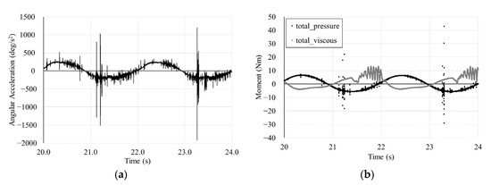
Figure 8.
(a) Angular acceleration and (b) total pressure and viscous moments of the flap-type wave energy converter.
As for the values for the radial acceleration, the CFD values show similar behaviour to that of the experimental tests, but they have a relative difference of approximately 10%. As the radial acceleration is related to the tangential acceleration results, the error of the latter is transferred and added to the results presented in Figure 7b. It is highly possible that this is the reason why the tangential acceleration results have a better match than the radial acceleration results.
To run the case, the NWT is divided into 108–240 subdomains, using the scotch decomposition method. The number of subdomains depends on the numbers of cells considered in the numerical domain. By using the scotch decomposition method, the programme balances the number of cells of each subdomain and its mesh complexity to be as close as possible to the other subdomains throughout the whole computational model [51]. The solution of the fluid problem was done within each subdomain which is assigned to one processor, and later assembled for the post-processing analysis. The study case using 240 processors (or subdomains) takes approximately 24 h to run 40 s (or 20 wave periods) of simulation, with a time-step adjusted to a maximum CFL of 0.65.
A similar validation process was done in [19] were the two-dimensional model performing under steep waves was compared to the experimental results obtained in Ecole Centrale Marseille (ECM) and further reported in [7]. For this study, [19], the domain discretised considered 550 CPW and 12 CPH, and the results validated were related to the motion of the device. The high-steep waves interacting with the OWSC caused the angular displacement to be higher than ±40 degrees (see Figure 9).
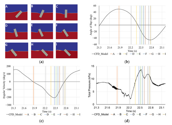
Figure 9.
Time series presenting one period of the OWSC movement: (a) Motion of the OWSC, (b) rotation angle of the OWSC, (c) angular velocity, and (d) total pressure measured at the contact point between the flap and the free surface in its upright position.
One period sequence of the simulation is shown in Figure 9, along with the results of the angle of rotation, angular velocities, and pressure. In Frame (A), the maximum rotation of the device is facing opposite to the wave generation patch, the angular velocity is zero, and the pressure measured in the contact surface of the flap at still water level is large. When the water runs down the flap, the pressure drops to zero in the absence of water in this region (see Frames (B) and (C)), whereas the negative angular velocity increases, and the flap returns to its initial position in Frame (C), where the rotation is 0. In Frame (D), the wave runs up the flap, the negative angular velocity reaches the minimum value, and the rotation of the flap changes the direction, to reach the largest angle in the seaward direction (Frame I), where the angular velocity is zero. The pressure loads acting on the flaps surface increases suddenly from Frames (E) to (F).
Nevertheless, for the present study, the three-dimensional model is the one used to add the PTO system, since the normal operating conditions for the device are under this regime of low-steep waves.
3.2. Power Capture
In an initial study undertaken in [52], the power capture of the Oyster was assessed by selecting the wave operating sea conditions of the device. These conditions represented 60% of the total occurrence of the sea as reported in [43]. Within these conditions, according to the results obtained, the performance of the device had the best performance, in terms of the CWR, when the full prototype operates with the higher wave periods considered (for this specific case, 7.5 and 8.5 s).
The approach undertaken in [52] involved a combination of damping control systems to model the PTO. In Figure 10, the results of the non-dimensional power capture against the non-dimensional wave frequency are plotted for different wave heights within a range of 0.02–0.06 m (corresponding to 0.80–2.40 m of the full-scale prototype). Despite that the energy carried by the sea waves is directly proportional to the wave height squared [29]; in this study, it was concluded that the influence of the wave height within the range considered is negligible compared to that of the wave period, as seen in Figure 10. In previous studies for undamped OWSC models, when increasing the wave amplitude, the amplitude of the oscillation of the flap is higher. However, in the same figure (Figure 10), it is shown than when considering the PTO, this is not a direct factor, but the combination of both the wave frequency and its height. Moreover, it is shown that the influence of the nonlinear effects is stronger for steeper waves, namely for higher wave heights, as the results are presented in non-dimensional form.
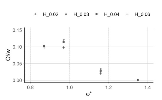
Figure 10.
Capture factor against the non-dimensional wave frequency for different wave heights for a 1:40 scale OWSC model.
In Figure 11a, the changes in the capture factor were compared using the wave height and frequency. Despite increasing the wave height, the variation in the capture factor appears to be minimum, compared to the effect of the variation of the wave frequency. To investigate this further, Figure 11b presents the motion response of the flap against different wave heights, but for the same wave period of 1.19 s. The motion response is given by the ratio of the angle of rotation of the flap and the amplitude of the wave, Aw. In this Figure, it can be noted that when considering the PTO, there is no direct relation between the amplitude motion of the OWSC and the wave height, because for a higher wave height, a lower angular motion can be obtained due to the influence of the nonlinear effects. In addition, it can be seen that the PTO influences in the time and phase shifts of the oscillatory motion of the WEC device, as the phase shift in the positive direction is weaker than that in the negative direction.
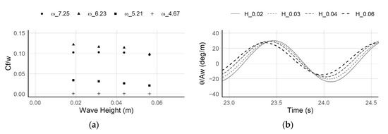
Figure 11.
(a) Capture factor against the wave heights for different wave frequencies studied; (b) motion response per wave amplitude for different a non-dimensional wave frequency of 0.97.
In the present study, the OWSC is studied by the influence of two control strategies, using reactive and passive controls, calculated for different wave periods, as it is described below.
3.2.1. Wave Resource
The wave parameters are scaled to a 1:40 model by using Froude scaling where the ratio for the wave height is equal to s (s is the scaling factor of 40) and for the period is s0.5. The values already scaled and used in this study for regular waves are shown in Table 3. The values considered correspond to a single wave height of 0.02 m with different periods:
Table 3.
Wave periods of the regular sea waves considered in the study.
The range of applicability of wave theories according to their height, period and depth was investigated in [53]. For the waves considered in the present work, and based on this range of applicability, it is recommended to use Stokes 2nd Order Waves.
3.2.2. Power Control
If the estimation of the PTO control in the model is oversimplified, the power capture calculation of the WEC device could lead to overestimated values [30]. To understand the influence of the PTO in the performance of the WEC device, two control systems are included; these strategies are the reactive and passive controls. For the general case, this PTO system is added as a restraint in the motion solution of the OWSC as an external moment:
where Bm is the mechanical damping coefficient, K the pitch stiffness coefficient, is the flap motion amplitude, and the angular velocity.
Whereas the undamped model means that and K are set to zero, for passive/resistive damping control, K remains zero and is matched to harness the maximum power capture for each wave condition considered. For this, the damping coefficient is derived from linear theory approach and set to an optimum value for each wave frequency ω:
where B is the radiation damping coefficient, C is the hydrostatic restoring coefficient, is the moment of inertia, and A is added moment of inertia. The hydrodynamic coefficients, B and A, are obtained from the curves given in [28]. The values of C and I are obtained for a simple plate assuming that its thickness is much smaller than its width and that the mass is uniformly distributed.
where t, h, and w are the thickness, height, and width of the plate, respectively. The water depth is d. The densities of the plate and the seawater are identified with the variables and , whilst the centre of buoyancy and centre of the mass of the flap by the variables and .
For the case of reactive control strategy, K is fixed that of a vertical plate [25], and :
Assuming the power is fully extracted by the PTO, the maximum absorbed power by the PTO is obtained with the following equations for reactive and passive controls, Equations (8) and (9), respectively [29]:
where is the maximum amplitude calculated from the numerical model and the power absorbed by the device when performing with passive control strategy is the maximum value of . Further, the estimation of the wave resource is defined as:
where k is the wave number.
The capture factor (Cf) is obtained from the ratio of the absorbed power and the available wave resource:
The unit of this ratio is meters and to non-dimensionalise it, it is related to the characteristic length of the device, the width, by using Cf/w.
Since this study is based on small-amplitude waves, the hydrodynamic coefficients calculated linearly in [28] are used to estimate the optimal damping coefficient for each wave frequency. To obtain the added moment of inertia, A, and the radiation damping coefficient, B, the non-dimensional angular frequency is used, ω*. This is obtained by the following equation:
Finally, Table 4 shows the values of the damping coefficients obtained used in the PTO moment added back to the motion equation.
Table 4.
Damping coefficients for each wave frequency of the study.
In the case of the results using passive control strategy for higher non-dimensional wave frequencies (cases CX01-03), divergent results were obtained. In the results of the angular displacement of the device, within these conditions, the restoring force is not high enough to allow the oscillation of the flap over its upright position, causing instability of the OWSC during the simulations. One possible explanation is that in these cases the moment imposed at the hinge by the PTO obtained using linear methods is misestimated. Therefore, there is a mismatch when integrating the linearised controller and the computational model, whose nonlinear effects, related to the calculation of the WEC’s surface forces, are increased when it operates under high wave frequencies. Nevertheless, for the full-scale prototype, this instability is not relevant since the device will operate under a regime where the period varies between 5 and 20 s (or the circular wave frequency varies between 0 and 4 rad/s) for meaningful energy extraction [54].
The results of the non-dimensional value, Cf/w, for both control strategies are shown in Figure 12, where the linear results of the OWSC are also presented for ratios between the flap’s thickness and the water depth of 0.1 and 0.2. The curves shown for the linear theory results are plotted using data taken from [28] for these specific conditions and for a non-dimensional wave frequency, ω*, range of 0.8–1.5. Despite that the OWSC studied here has a ratio of t/d = 0.30, the non-linear viscous effects seem to be highly important when calculating the value of the non-dimensional frequency to which the ratio of the power captured by the device is higher.
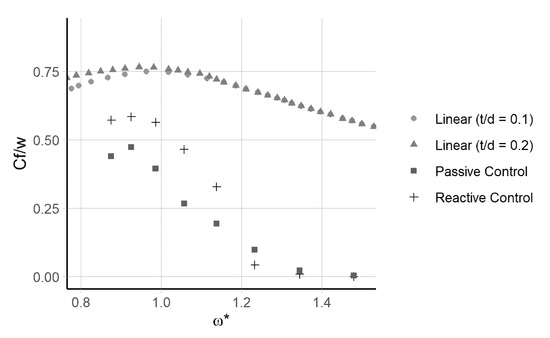
Figure 12.
Capture factor against the non-dimensional wave frequency for reactive and passive control strategies using linear and nonlinear approach. The linear theory results are for damping control systems (adapted from [28]).
Moreover, for higher frequencies, i.e., when the waves are steeper, the linear method approach differs from non-linear approach (see Figure 12). One factor to bear in mind is that the assumption of small thickness compared to its width, used in linear theory, may not be applicable when calculating the hydrodynamic coefficients, suggesting that additional nonlinear methods should be sought to calculate them.
The results for the power generated in (W) are presented for both the reactive and resistive control simulations, in Figure 13. As a comparison, the results of cases CX07 and CX08 are included in both graphics, since these are related to the high power capture factor Cf/w obtained. Whilst for the reactive control system there are some negative values, it can be found that with this control system under the same wave conditions, the power capture by the WEC would be higher.
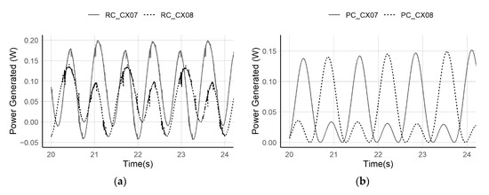
Figure 13.
(a) Power generated for cases CX07-CX08 using reactive control; (b) power generated for cases CX07-CX08 using passive control.
3.3. Wave Pattern
In this section, the case with the highest Cf/w, CX07, is used for the investigations of the analysis of the wave flow around the flap. In Figure 14, the relative wave surface elevation in the NWT of this case is presented at three positions of the flap. Figure 14a is when the flap is at its maximum amplitude towards the land, Figure 14b at its upright position, and Figure 14c at its maximum amplitude towards the sea. In (a), the wave height towards the side of the flap is increased, as well as an additional wave radiated from the device. In the case of (b), when the wave field faces the upright flap as a fixed object, the diffracted wave shape can be appreciated on the sides by its change in the relative wave height. As in the case of (c), it is similar to the case of (a), but the radiated wave is towards the sea, where it can be seen that the reflected waves considerably damped the incident waves.
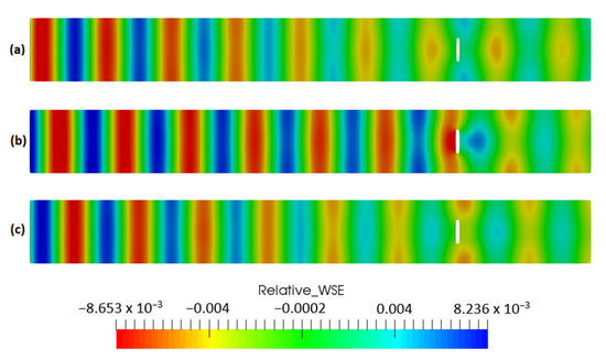
Figure 14.
Relative wave surface elevation when the flap is at three different positions: (a) Maximum oscillation (landwards), (b) upright position, and (c) minimum oscillation (seawards).
This finding, while preliminary, suggests that this disturbance is not significant in the effective power capture of the OWSC operating as a single unit. However, it can imply that when considering devices operating in array configurations, it is of interest to understand the extent of the disturbed field. In this specific wave condition, it implies that the minimum location for a second device will be as its distance from the inlet (>12.20 m), which for this case would mean four times the wavelength used. Conversely, for the transverse direction, the NWT should require an extension in its width, to have a clearer appraisal of the behaviour of the diffracted waves.
4. Conclusions
Based on OpenFOAM, this study set out to determine the power capture absorbed by an OWSC device combined with two PTO control strategies modelled using a damper and spring-damper system. The model used in this study was first validated for an undamped device operating under first order waves against experimental tests. After comparing the numerical and experimental results, abnormal pressure peak values were observed, when the flap reaches its maximum angular displacement. For validation purposes, it was concluded that these effects did not influence the prediction of the total forces and position. Nonetheless, it would be worth to investigate if these effects are linked to additional wave loads or to numerical instabilities.
For this study, different wave periods of the site of operation of the full-scale prototype at a constant wave height were investigated. To calculate the power capture by each PTO system, the damping coefficients and spring coefficient were calculated for each wave frequency. It was found that, with the PTO taken into consideration, the relationship of power capture is no longer positively correlated with the incident wavelength; instead, an optimal wave condition exists. Moreover, it is also found that the damping and spring coefficients calculated may be overestimated for high frequency waves. This may suggest that for these cases the hydrodynamic coefficients should be calculated using an additional nonlinear approach.
The efficiency of the energy extracted from the waves is related to high-amplitude pitching motions of the device in short periods of time, as well as the capacity of the PTO to absorb the wave energy. Consequently, the incident wave field is disturbed due to the interaction with the flap and its motion. It is expected that the modified wave field caused by the motion of the OWSC becomes more relevant when it is performing in arrays with neighbouring devices. Future work will place multiple devices in a simulation to investigate the interaction between near OWSCs and then suggest arrangement strategies. It is also suggested that the response surface of a device in variable wave conditions should be built up, with the consideration of PTO, and this is recommended to combine with the Machine Learning technique to handle the large amounts of data [55].
Author Contributions
Conceptualization, D.B.-M., L.H., and G.T.; methodology, D.B.-M., J.R.M.-L., L.H., E.A., and G.T.; software, D.B.-M. and L.H.; validation, D.B.-M.; formal analysis, D.B.-M., L.H., and E.A.; writing—original draft preparation, D.B.-M.; writing—review and editing, D.B.-M., L.H., J.R.M.-L., E.A., and G.T. All authors have read and agreed to the published version of the manuscript.
Funding
The first author would like to acknowledge the financial support provided by the National Secretary of Higher Education, Science, Technology and Innovation (SENESCYT) and the Escuela Superior Politécnica del Litoral (ESPOL) of Ecuador.
Acknowledgments
Thanks go to Abbas Dashtimanesh for his editor contribution in this special issue. The authors acknowledge the use of the UCL Grace High Performance Computing Facility (Grace@UCL), and associated support services, in the completion of this work.
Conflicts of Interest
The authors declare no conflict of interest.
References
- Babarit, A. A database of capture width ratio of wave energy converters. Renew. Energy 2015, 80, 610–628. [Google Scholar] [CrossRef]
- Cameron, L.; Doherty, K.; Doherty, R.; Henry, A.; Hoff, J.V.; Kaye, D.; Naylor, D.; Bourdier, S.; Whittaker, T. Design of the Next Generation of the Oyster Wave Energy Converter. In Proceedings of the 3rd International Conference on Ocean Energy, Bilbao, Spain, 6–7 October 2010; pp. 1–12. [Google Scholar]
- Dhanak, M.; Xiros, N.I. (Eds.) Springer Handbook of Ocean Engineering; Springer: Berlin, Germany, 2016. [Google Scholar]
- Henry, A.; Doherty, K.; Cameron, L.; Whittaker, T.; Doherty, R. Advances in the Design of the Oyster Wave Energy Converter. In Proceedings of the Marine Renewable and Offshore Wind Energy Conference, Royal Institution of Naval Architects, London, UK, 21–23 July 2010. [Google Scholar]
- Folley, M.; Whittaker, T.; Henry, A. The effect of water depth on the performance of a small surging wave energy converter. Ocean Eng. 2007, 34, 1265–1274. [Google Scholar] [CrossRef]
- Schmitt, P.; Elsaesser, B. On the use of OpenFOAM to model oscillating wave surge converters. Ocean Eng. 2015, 108, 98–104. [Google Scholar] [CrossRef]
- Henry, A.; Kimmoun, O.; Nicholson, J.; Dupont, G.; Wei, Y.; Dias, F. A two dimensional experimental investigation of slamming of an Oscillating Wave Surge Converter. In Proceedings of the Twenty-Fourth International Ocean and Polar Engineering Conference, Busan, Korea, 15–20 June 2014; pp. 296–305. [Google Scholar]
- Henry, A.; Abadie, T.; Nicholson, J.; McKinley, A.; Kimmoun, O.; Dias, F. The Vertical Distribution and Evolution of Slam Pressure on an Oscillating Wave Surge Converter. In Proceedings of the ASME 2015 34th International Conference on Offshore Mechanics and Arctic Engineering, St. John’s, NL, Canada, 31 May–5 June 2015; pp. 1–11. [Google Scholar]
- Renzi, E.; Dias, F. Hydrodynamics of the oscillating wave surge converter in the open ocean. Eur. J. Mech. B/Fluids 2013, 41, 1–10. [Google Scholar] [CrossRef]
- Renzi, E.; Doherty, K.; Henry, A.; Dias, F. How does Oyster work? The simple interpretation of Oyster mathematics. Eur. J. Mech. B/Fluids 2014, 47, 124–131. [Google Scholar] [CrossRef]
- Rafiee, A.; Elsaesser, B.; Dias, F. Numerical Simulation of Wave Interaction With an Oscillating Wave Surge Converter. In Proceedings of the ASME 2013 32nd International Conference on Ocean, Offshore and Arctic Engineering, Nantes, France, 9–14 June 2013. [Google Scholar]
- Brito, M.; Canelas, R.; García-Feal, O.; Domínguez, J.; Crespo, A.J.C.; Ferreira, R.; Neves, M.G.; Teixeira, L. A numerical tool for modelling oscillating wave surge converter with nonlinear mechanical constraints. Renew. Energy 2020, 146, 2024–2043. [Google Scholar] [CrossRef]
- Huang, L.; Ren, K.; Li, M.; Tuković, Ž.; Cardiff, P.; Thomas, G. Fluid-structure interaction of a large ice sheet in waves. Ocean Eng. 2019, 182, 102–111. [Google Scholar] [CrossRef]
- Huang, L.; Thomas, G. Simulation of Wave Interaction With a Circular Ice Floe. J. Offshore Mech. Arct. Eng. 2019, 141, 041302. [Google Scholar] [CrossRef]
- Huang, L.; Li, M.; Romu, T.; Dolatshah, A.; Thomas, G. Simulation of a ship operating in an open-water ice channel. Ships Offshore Struct. 2020, 1–10. [Google Scholar] [CrossRef]
- Huang, L.; Tuhkuri, J.; Igrec, B.; Li, M.; Stagonas, D.; Toffoli, A.; Cardiff, P.; Thomas, G. Ship resistance when operating in floating ice floes: A combined CFD&DEM approach. Mar. Struct. 2020, 74, 102817. [Google Scholar] [CrossRef]
- Ferrer, P.J.M.; Qian, L.; Ma, Z.; Causon, D.M.; Mingham, C.G. Improved numerical wave generation for modelling ocean and coastal engineering problems. Ocean Eng. 2018, 152, 257–272. [Google Scholar] [CrossRef]
- Wei, Y.; Abadie, T.; Henry, A.; Dias, F. Wave interaction with an Oscillating Wave Surge Converter. Part I: Viscous effects. Ocean Eng. 2015, 104, 185–203. [Google Scholar] [CrossRef]
- Benites-Munoz, D.; Huang, L.; Thomas, G. The interaction of cnoidal waves with oscillating wave surge energy converters. In Proceedings of the 14th OpenFOAM Workshop, Duisburg, Germany, 23–26 July 2019. [Google Scholar]
- Windt, C.; Davidson, J.; Ringwood, J.V. High-fidelity numerical modelling of ocean wave energy systems: A review of computational fluid dynamics-based numerical wave tanks. Renew. Sustain. Energy Rev. 2018, 93, 610–630. [Google Scholar] [CrossRef]
- ITTC. The Specialist Committee on Hydrodynamics Modelling of Marine Renewable Energy Devices. In Proceedings of the 28th ITTC—Volume II Final Report and Recommendations to the 28th ITTC; ITTC: Lawrence, KS, USA, 2017. [Google Scholar]
- Wave Energy Scotland, “Power Take-Off Projects”. Available online: https://www.waveenergyscotland.co.uk/programmes/details/power-take-off/ (accessed on 10 July 2020).
- Zhang, D.-H.; Li, W.; Zhao, H.-T.; Bao, J.-W.; Lin, Y.-G. Design of a hydraulic power take-off system for the wave energy device with an inverse pendulum. China Ocean Eng. 2014, 28, 283–292. [Google Scholar] [CrossRef]
- Brito, M.; Teixeira, L.; Canelas, R.B.; Ferreira, R.; Neves, M.G. Experimental and Numerical Studies of Dynamic Behaviors of a Hydraulic Power Take-Off Cylinder Using Spectral Representation Method. J. Tribol. 2017, 140, 021102. [Google Scholar] [CrossRef]
- Behzad, H.; Panahi, R. Optimization of bottom-hinged flap-type wave energy converter for a specific wave rose. J. Mar. Sci. Appl. 2017, 16, 159–165. [Google Scholar] [CrossRef]
- Bacelli, G.; Genest, R.; Ringwood, J.V. Nonlinear control of flap-type wave energy converter with a non-ideal power take-off system. Annu. Rev. Control. 2015, 40, 116–126. [Google Scholar] [CrossRef]
- Senol, K.; Raessi, M. Enhancing power extraction in bottom-hinged flap-type wave energy converters through advanced power take-off techniques. Ocean Eng. 2019, 182, 248–258. [Google Scholar] [CrossRef]
- Gomes, R.; Lopes, M.; Henriques, J.; Gato, L.; Falcão, A. The dynamics and power extraction of bottom-hinged plate wave energy converters in regular and irregular waves. Ocean Eng. 2015, 96, 86–99. [Google Scholar] [CrossRef]
- Falnes, J. Ocean Waves and Oscillating Systems; Cambridge University Press: Cambridge, UK, 2004. [Google Scholar]
- Penalba, M.; Davidson, J.; Windt, C.; Ringwood, J.V. A high-fidelity wave-to-wire simulation platform for wave energy converters: Coupled numerical wave tank and power take-off models. Appl. Energy 2018, 226, 655–669. [Google Scholar] [CrossRef]
- Schmitt, P.; Asmuth, H.; Elsaesser, B. Optimising power take-off of an oscillating wave surge converter using high fidelity numerical simulations. Int. J. Mar. Energy 2016, 16, 196–208. [Google Scholar] [CrossRef]
- Windt, C.; Ringwood, J.V.; Davidson, J.; Ransley, E.J.; Jakobsen, M.; Kramer, M. Validation of a CFD-based numerical wave tank of the Wavestar WEC. In Proceedings of the 3rd International Conference on Renewable Energies Offshore, Lisbon, Portugal, 8–10 October 2018. [Google Scholar]
- Devolder, B.; Stratigaki, V.; Troch, P.; Rauwoens, P. CFD Simulations of Floating Point Absorber Wave Energy Converter Arrays Subjected to Regular Waves. Energies 2018, 11, 641. [Google Scholar] [CrossRef]
- Cruz, J. Ocean Wave Energy: Current Status and Future Prespectives; Springer: Berlin, Germany, 2008. [Google Scholar]
- Wei, Y.; Abadie, T.; Henry, A.; Dias, F. Wave interaction with an Oscillating Wave Surge Converter. Part II: Slamming. Ocean Eng. 2016, 113, 319–334. [Google Scholar] [CrossRef]
- Hirt, C.; Nichols, B. Volume of fluid (VOF) method for the dynamics of free boundaries. J. Comput. Phys. 1981, 39, 201–225. [Google Scholar] [CrossRef]
- Ferziger, J.H.; Peric, M.; Street, R.L. Computational Methods for Fluid Dynamics; Springer: Berlin, Germany, 2002. [Google Scholar]
- Jasak, H. Error Analysis and Estimation for the Finite Volume Method with Applications to Fluid Flows. Ph.D. Thesis, Imperial College, London, UK, 1996. [Google Scholar] [CrossRef]
- Moukalled, F.; Mangani, L.; Darwish, M. The Finite Volume Method in Computational Fluid Dynamics; Springer: Berlin, Germany, 2016. [Google Scholar]
- Rusche, H. Computational Fluid Dynamics of Dispersed Two-Phase Flows at High Phase Fractions. Ph.D. Thesis, University of London, London, UK, 2002. [Google Scholar] [CrossRef]
- Higuera, P.; Lara, J.L.; Losada, I.J. Realistic wave generation and active wave absorption for Navier–Stokes models. Coast. Eng. 2013, 71, 102–118. [Google Scholar] [CrossRef]
- IHCantabria. IHFOAM Manual. 15 July 2014. [Google Scholar]
- O’Boyle, L.; Doherty, K.; van’t Hoff, J.; Skelton, J. The Value of Full Scale Prototype Data—Testing Oyster 800 at EMEC, Orkney. In Proceedings of the 11th European Wave and Tidal Energy Conference (EWTEC), Nantes, France, 6–11 September 2015; pp. 1–10. [Google Scholar]
- Windt, C.; Davidson, J.; Chandar, D.D.J.; Ringwood, J.V. On the Importance of Advanced Mesh Motion Methods for WEC Experiments in CFD-based Numerical Wave Tanks. In Proceedings of the VIII International Conference on Computational Methods in Marine Engineering, Gothenburg, Sweden, 13–15 May 2019; pp. 145–156. [Google Scholar]
- Chan, W.; Gomez, R.; Rogers, S.; Buning, P. Best Practices in Overset Grid Generation. In Proceedings of the 32nd AIAA Fluid Dynamics Conference and Exhibit, St. Louis, MO, USA, 24–26 June 2002. [Google Scholar]
- Newmark, N.M. A method of computation for structural dynamics. J. Eng. Mech. Div. 1959, 85, 67–94. [Google Scholar]
- Pai, P. Highly Flexible Structures: Modeling, Computation, and Experimentation; American Institute of Aeronautics and Astronautics: Reston, VA, USA, 2007. [Google Scholar]
- Buchholdt, H.A.M.; Nejad, S.E. Response of linear and non-linear one degree-of-freedom systems to random loading: Time domain analysis. In Structural Dynamics for Engineers, 2nd ed.; Thomas Telford: London, UK, 2012; pp. 117–135. [Google Scholar]
- ITTC. Uncertainty Analysis in CFD Verification and Validation, Methodology and Procedures; ITTC: Lawrence, KS, USA, 2008. [Google Scholar]
- Stern, F.; Wilson, R.V.; Coleman, H.W.; Paterson, E.G. Comprehensive Approach to Verification and Validation of CFD Simulations—Part 1: Methodology and Procedures. J. Fluids Eng. 2001, 123, 793–802. [Google Scholar] [CrossRef]
- OpenFOAM ESI. The Open Source CFD Toolbox, no. Version v1906. 2019. [Google Scholar]
- Benites-Munoz, D.; Huang, L.; Anderlini, E.; Thomas, G. Simulation of the wave evolution and power capture of an oscillating wave surge converter. In Proceedings of the 30th International Ocean and Polar Engineering Conference, Shanghai, China, 11–16 October 2020. [Google Scholar]
- Méhauté, B. An Introduction to Hydrodynamics and Water Waves; Springer: Berlin/Heidelberg, Germany, 1976. [Google Scholar]
- Holthuijsen, L.H. Waves in Oceanic and Coastal Waters; Cambridge University Press: Cambridge, UK, 2007. [Google Scholar]
- Anderlini, E. Control of wave energy converters using machine learning strategies. Ph.D Thesis, Industrial Doctorate Centre for Offshore Renewable Energy (IDCORE), Edinburgh, UK, 2017. [Google Scholar]
© 2020 by the authors. Licensee MDPI, Basel, Switzerland. This article is an open access article distributed under the terms and conditions of the Creative Commons Attribution (CC BY) license (http://creativecommons.org/licenses/by/4.0/).