Modulated Response of Subtropical Gyres: Positive Feedback Loop, Subharmonic Modes, Resonant Solar and Orbital Forcing

Abstract

Evidence of long-term variability in the upper ocean has emerged for two decades. Most of the issues discussed raise a lot of questions. What is the driver of the decadal oscillation of rainfall in Europe that has been observed since the end of the 20th century? How to explain low-frequency variability as observed in the Atlantic Multidecadal Oscillation (AMO)? More generally, how does solar and orbital forcing occur during very long-term climate change? The observations suggest that both a positive feedback loop amplifies the effects of the insolation gradient on the climate system and a resonance phenomenon occurs, filtering out some frequencies in favour of others. Throughout this paper, some answers to these problems are given from a new concept based on the modulated response of subtropical gyres to solar and orbital forcing. Subtropical gyres turn out to be the main driver of long-term climate variability because they tightly control, via the western boundary currents, heat transport from the tropics into middle and high latitudes. Specifically, the theoretical foundations of long-period Rossby waves winding around the subtropical gyres are laid, suggested by the observations of persistent sea surface temperature anomalies at mid-latitudes. Multi-frequency Gyral Rossby Waves (GRWs) exhibit properties resulting from their annular structure and their coupling. Using a β-cone approximation, the momentum equations are solved in polar coordinates. The gradient β of the Coriolis parameter depends on the mean radius of the annulus and remains constant all around the latter. GRWs result from the variation in the Coriolis Effect with the mean radius of the annulus. The speed of the anti-cyclonically wind-driven circulation being higher than the phase velocity of cyclonically propagating GRWs, amplified forcing effects occur as well as resonances for periods consistent with the observations.

1. Introduction

Evidence of mid-latitude long-term variability in the upper ocean has emerged for two decades: in the North Atlantic [1], in the North Pacific [2,3,4,5] and in the South Pacific [6,7]. Because the oceanic circulation above the thermocline is primarily wind-driven, a simple explanation of this low-frequency variability is that the ocean responds linearly and passively to random atmospheric wind forcing [8]. Cessi and Louazel [9] developed a linear model to show how the upper ocean dynamics filter stochastic atmospheric forcing to produce decadal variability. The decadal response of the ventilated thermocline to surface buoyancy forcing was investigated by Czaja and Frankignoul [10] the decadal forcing being represented as a slow modulation of the seasonal cycle, rather than a slow periodic forcing as in Liu and Pedlosky [11]. Considering basins with a large variation of the Coriolis parameter, significant progress was obtained in understanding the decadal variability of the upper oceans at mid-latitudes when shallow-water equations with weak friction are calculated numerically or using an analytic approximation, enforcing boundary conditions at the western limit of the basin.

1.1. Long-Term Variability of the Upper Ocean

Most of the issues discussed raise a lot of questions as concerns the driver of the decadal oscillation of rainfall in Europe, the low-frequency variability of the upper oceans as observed in the Atlantic Multidecadal Oscillation (AMO) as well as the solar and orbital forcing that occur during very long-term climate change. The latter requires the ocean circulation is driven by the Earth latitudinal temperature gradient as showed by Davis and Brewer [12,13]. Furthermore, the impact of orbital parameters on climate seems not proportional to the amplitude of the resulting solar irradiance variations. Over the past 800,000 years, the period of oscillation of glacial-interglacial that dominated is 100,000 years, showing it is mainly subject to the eccentricity parameter. During the interval from 3.0 to 0.8 million years before our era, the period of 41,000 years prevailed, corresponding to changes in the obliquity of the Earth, what is named the transition problem.

The observations suggest that both a positive feedback loop amplifies the effects of the insolation gradient on the climate system and a resonance phenomenon occurs, filtering out some frequencies in favour of others. These hypotheses, issued for several decades, arise huge problems and there is currently no consensus on the responsible mechanism. These aspects of climatology are, however, of the utmost importance in the current context of climate change.

1.2. The Role of Subtropical Gyres

Throughout this paper, some answers to these problems are given from a new concept based on the modulated response of subtropical gyres. We will investigate the role of the latter that are the main driver of long-term variability of climate because they tightly control, via the western boundary currents, heat transport from the tropics into middle and high latitudes. For that, the variability of the upper ocean at mid-latitudes will be focused on the response of subtropical gyres to solar and orbital forcing.

Due to the western boundary of the basin, the formation of westward-propagating Rossby waves at mid-latitudes, as observed by many authors (e.g., [9]), requires the westward phase velocity of the Rossby waves be lower than the eastward velocity of the wind-driven circulation in which they are embedded. The resulting waves propagate eastward with an apparent phase velocity −ω/k’ where −k’ is the apparent wavenumber; ω = 2π/T where T is the period.

Western boundary currents have the potential ability to convey a succession of warm water masses at particular frequencies, thus producing the deepening or the rising of the thermocline where they leave the continents to enter the subtropical gyres. A resonance occurs when the apparent wavelengths of the embedded non-dispersive Rossby waves are adjusted in order to tune their natural period to the forcing period.

Resonantly forced baroclinic waves at mid-latitudes are quasi-stationary waves whose average periods are 1/2-, 1-, 4- and 8-years [14]. They can be observed using the cross-wavelet analysis of the Sea Surface Height (SSH) and the geostrophic Surface Current Velocity (SCV). Both SSH and SCV anomalies are related within the hypothesis of a quasi-geostrophic motion.

Quasi-stationary waves exhibit western and eastern SSH anomalies in opposite phases, as well as western and eastern modulated SCV anomalies also in opposite phases: the western SSH anomalies stretch along the gyres whereas the eastern SSH anomalies are outside the gyre, escaping poleward [14]. They merge either with the North Atlantic Drift, or the North Pacific Drift, or the Antarctic circumpolar currents in the southern hemisphere according to the five subtropical gyres.

In this case, the western SSH and SCV anomalies are opposite. In such condition, the western SSH anomaly takes the place of the eastern SSH anomaly after half a cycle, while a new western SSH anomaly is formed, in opposite phase versus the previous one. This leads to the transfer poleward and outside the gyres of successive warm water masses.

Starting from the properties of short-period resonantly forced Rossby waves dragged by the wind-driven circulation [14], we will explore under what conditions they can wrap around the gyres when their period increases. Within this context, Rossby waves no longer result from the variation in the gradient of the Coriolis parameter β versus the latitude but from the variation of the gradient expressed in relation to the mean radius of the gyre.

The annular representation of the resonantly forced Rossby waves gives them particular properties. At first, they propagate cyclonically around the annulus. Since their phase velocity is lower than the anticyclonic speed of the steady wind-driven current, the apparent phase velocity of the embedded Rossby wave is anticyclonic.

As for short-period resonantly forced waves, a subharmonic mode locking occurs because multi-frequency Rossby waves share the same modulated geostrophic current around the gyre [14]. But here the conditions of resonance are subject to an additional constraint: half the apparent wavelength of the embedded Rossby waves must equal $N$ times the circumference of the median line of the gyre. The phase velocity of Rossby waves depends on the location of the centroid of the gyre, exclusively. Therefore, this location plays a particular role in the tuning of the resonance conditions.

While the apparent wavelength of the short-period resonantly forced waves sets their period, it is the number of turns made around the gyre before leaving it which defines the period of the annular Rossby waves, each of them behaving like a coupled oscillator. When the resonance conditions are satisfied, the component of the pycnocline depth oscillation associated with such an oscillator deepens during half a period whereas it rises outside the gyre. The contrary occurs during the following half period so that such progressive waves behave like quasi-stationary waves.

These are the properties of such annular Rossby waves that we propose to study in the context of this paper which follows a work on multi-frequency short-period Rossby waves considered as coupled oscillators ruled by the Caldirola-Kanai equation [14]. Extrapolation of properties of Rossby waves to annular structure allows us to approach the dynamics of subtropical gyres in a new way. Focused on long-period resonantly forced waves, the results mainly concern the North Atlantic for which long series of data can be used reliably.

2. Method

2.1. The Annular Representation of Baroclinic Waves

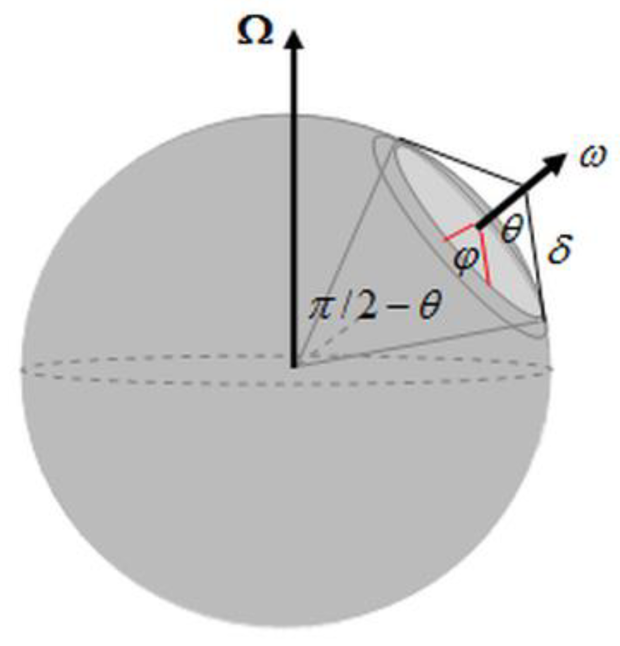
The long-period Rossby waves propagate over a significant range of latitudes around the subtropical gyres, which invalidates the β-plane approximation for which the north-south scale must be small enough for changes in $f$ to be small over such a distance. Moreover, the Cartesian coordinates in the β-plane, that is, the longitude and latitude $x$ and $y$ are no longer suited to the study of gyres. In this case, the approximation of the β-cone is required (Figure 1). A cone of revolution tangent to the terrestrial sphere defines a circle $C$ common to the cone and the sphere. To make this circle as close as possible to the median line of the gyre, the axis of the cone passes through the center of gravity (the centroid) of the gyre; its apex angle θ is defined so that the radius of the circle C equals the average radius of the gyre.

In conical coordinates $x=\delta \sin \theta \cos \phi$, $y=\delta \sin \theta \sin \phi$, $z=\delta \cos \theta$ (δ is the distance to the apex of the cone, φ is the polar coordinate). Consider an orthogonal system of reference whose axis $z$ coincides with the axis of the cone and whose abscissa axis is tangent to the circle $C$. This system is rotated about the axis $z$ with uniform angular velocity $\overrightarrow{\omega }=\overrightarrow{f_0}/2$: $\overrightarrow{\omega }$ is the projection of the vector of rotation of the earth $\overrightarrow{\Omega }$ on the axis of the cone; the Coriolis parameter $f_0$ (the norm of $\overrightarrow{f_0}$) is $f_0=2\Omega \sin {\phi }_0$ where ${\phi }_0$ is the latitude of the centre of the circle $C$.

As this is done to derive the quasi-geostrophic momentum equations under the mid-latitude β-plane approximation when the central point is far more than a Rossby radius from the equator (the distance for which the effects of rotation are important, of the order of 2000 km), the momentum equation for a material element located on the circle $C$ is:

$$D\overrightarrow{u}/Dt+\overrightarrow{f}\times \overrightarrow{u}=-{\rho }^{-1}\nabla p+forcing$$

(1)

where ρ is the density of sea water and $\nabla p$ the pressure gradient. The Coriolis vector $\overrightarrow{f}$ is 2 times the vector of rotation at the location of the material element (the projection of $\overrightarrow{f_0}$ onto the vertical). The Coriolis parameter $f$ (the norm of the Coriolis vector $\overrightarrow{f}$), is constant around the circle $C$ so that $f=f_0\sin \theta$.

Given the motion of the material element, the gradients of the coordinates $u$, $v$ and $w$ of the velocity vector $\overrightarrow{u}$ are supposed to be small such that a uniform translation can be hypothesized locally: $D\overrightarrow{u}/Dt=\partial \overrightarrow{u}/\partial t$. Now, let us assume that the surface elevation $z=\eta$ relative to a geopotential surface is small to consider the hydrostatic approximation. Using the polar coordinate φ on the circle $C$ whose radius is $r$ and the distance δ to the apex of the cone, the momentum equations of two superposed fluids of different density are (the first baroclinic mode is assumed but the results can be simply extended to higher normal baroclinic modes $n$, $H_1$, $H_2$ … representing the depth of the successive interfaces and $c_n$ the phase speed associated with the mode):

$$\partial u/\partial t-fv=-g\partial \eta /\partial \left(r\phi \right)+X/{\rho }_1{H}_1$$

(2)

$$\partial v/\partial t+fu=-g\partial \eta /\partial \delta +Y/{\rho }_1{H}_1$$

(3)

where $u$ and $v$ are the coordinates of the velocity vector $\overrightarrow{u}$ in the orthogonal system: $u$ is the polar current and $v$ the radial current. η is the perturbation of the surface height and $h$ the displacement of the interface upwardly resolved in vertical mode: $\mu =\eta /h=-g’H_2/gH$, $g^{\prime }=g\left(1-{\rho }_1/{\rho }_2\right)$. $H_1$ is the depth of the upper layer, $H_2$ is the depth of the lower layer and $H=H_1+H_2$ is the total depth. ${\rho }_1$ and ${\rho }_2$ are the density of the upper and the lower layer, respectively. $X$ and $Y$ are the surface stress forcing terms relative to the polar coordinate φ and the distance δ to the apex of the cone, respectively.

Therefore, the quasi-geostrophic momentum equations remain virtually the same as those referring to the β-plane approximation but now the Coriolis parameter $f$ is constant around the circle $C$, depending only on the radius. The variation of the Coriolis parameter $f$ versus δ is obtained by considering secant planes parallel to $C$: they define circles at the intersections with the sphere. If $\delta \cos \theta$ is the distance of such a circle to the apex of the cone, the Coriolis vector $\overrightarrow{f}$ around the circle is still obtained by projecting $\overrightarrow{f_0}$ onto the vertical. Thus, the Coriolis parameters around concentric circles on the sphere only depend on δ. Furthermore, the gradient of the Coriolis parameter is $\beta =\left(2\Omega /R\right)\cos {\phi }_0$. The β-cone approximation relies on expanding $f$ versus δ and is obtained just as it is for the β-plane for which $f$ is a linear function of $y$: $f=f_0+\beta \delta$.

The equation of continuity on the surface of the cone is:

$$\partial \eta /\partial t+H_1\mathrm{div}\overrightarrow{u}=-E/{\rho }_1$$

(4)

where $E$ is the evaporation rate and: $\mathrm{div}\overrightarrow{u}=\frac{r}{\delta \sin \theta }\partial u/\partial \left(r\phi \right)+\frac{1}{{\delta }^2}\partial \left({\mathsf{\delta }}^2\mathrm{v}\right)/\partial \delta$; So $\mathrm{div}\overrightarrow{u}\approx \partial u/\partial \left(r\phi \right)+\partial v/\partial \delta$ in the vicinity of the circle $C$.

To remove the inconsistency that would arise if forcing terms resulted in nonzero divergence, the equation of vorticity is added, that is:

$$\frac{\partial }{\partial t}\left(\xi -f\eta /H_1\right)+\beta v=\frac{1}{{\rho }_1{H}_1}\left(r\partial Y/\partial \left(r\phi \right)-\partial X/\partial \delta +fE\right)$$

(5)

where $\xi -f\eta /H_1$ is the absolute vorticity. The relative vorticity $\xi =\frac{r}{\delta \sin \theta }\partial v/\partial \left(r\phi \right)-\frac{1}{\mathsf{\delta }}\partial \left(\delta u\right)/\partial \delta$ is the component of the curl of velocity $\overrightarrow{u}$ ($\mathrm{curl}\overrightarrow{u}$) perpendicular to the surface of the cone at the considered location. So $\xi \approx \partial v/\partial \left(r\phi \right)-\partial u/\partial \delta$ in the vicinity of the circle $C$.

Under the β-cone approximation, the equations of motion along closed convex paths are virtually unchanged in the vicinity of the circle $C$. Actually, the solution of the equations of motion is still valid when $x$ (the longitude) is defined from the polar coordinate $x\leftrightarrow r\phi$ and when $y$ (the latitude) represents the distance to the apex of the cone $y\leftrightarrow \delta$. In particular, the dispersion relation is still available, that is, in the case of long planetary waves, approximated by:

$$\omega /k=-\beta c^2/f_0^2=-c^2\cos {\phi }_0/2\mathsf{\Omega }R{\sin }^2{\phi }_0$$

(6)

where $c$ is the phase velocity along the equator for the first baroclinic mode. Furthermore, the resonance conditions are preserved. Like in [15,16,17] the coefficients and the forcing terms are expanded in parabolic cylinder functions for the latitude and in Fourier series for the longitude and time. The terms of Fourier series exhibit singularities, highlighting resonances and the relation between the resonance frequencies, that is, the forcing frequencies and the wavenumbers. This ill-posed problem is regularized by considering the Rayleigh friction.

2.2. The Wavelet Analysis

A cross-wavelet analysis [14,18] is preferred to a complex EOF analysis to investigate the Sea Surface Height (SSH) anomalies, the modulated geostrophic current velocity field and SST anomalies in a predetermined frequency band. If the two methods are similar for typical frequency domain analyses, that is, the power spectral and coherency analyses, they are far different in terms of the time domain. In complex EOF analysis the time lag between time series is basically the computation of eigenvector and eigenvalue of a covariance or a correlation matrix computed from a group of original time series data. In contrast, the cross-wavelet analysis is well suited to highlight the time lag between time series when it varies continuously.

Maps are paired, the first is the amplitude of anomalies (regardless of the time when the maximum anomaly occurs) and the second is the phase (the time evolution, that is, the time when the maximum anomaly occurs over a period). The band over which both the cross-wavelet power and the coherence phase are scale-averaged allows taking into account the natural broadening of the frequency bands associated with the oscillations. On both maps, the values at each pixel are processed independently of each other. Therefore, classes are chosen judiciously in relation to the observed random errors so as to confer the displayed anomalies a spatial continuity.

2.3. Antinodes and Nodes of Quasi-Stationary Waves

By representing the amplitude and phase of SSH and SCV anomalies, the cross-wavelet analysis highlights quasi-stationary waves characterized by antinodes at the SSH anomalies and nodes associated with the resulting modulated geostrophic current velocity, supposing a quasi-geostrophic motion. This terminology is convenient for describing quasi-periodic anomalies as opposed to incidental anomalies.

2.4. Subharmonic Modes

Gyral Rossby Waves (GRWs) sharing the same node around a gyre, they have to be considered as coupled oscillators ruled by the Caldirola-Kanai equation: the CK oscillator is a fundamental model of dissipative systems that is usually used for the damped harmonic oscillator. The coupling results from the alteration of the geostrophic forces of the basin as a consequence of the convergence and the merging of geostrophic currents [14].

Consequently, the periods are derived by induction so that:

$$T_i=n_i{T}_{i-1 },\times T_0=1yr$$

(7)

where $n_i$ is an integer higher than 1 [14]. The integer $n_i$ should be as small as possible to ensure the stability of the multi-frequency system of GRWs. Mostly, $n_i$ is 2 so that it is convenient to scale-average the wavelet power and the coherence phase within contiguous regions included between $3/4T_i$ and $3/2T_i$.

The annular structure of resonantly forced Rossby waves around the gyres give them particular properties. The term ‘gyral’ recalls that these are baroclinic waves behaving like coupled oscillators. The existence of cyclonic GRWs is closely related to the anticyclonic wind-driven circulation around the gyre. The speed of the steady wind-driven current is higher than the phase velocity of the Rossby wave that remains constant around the gyre as it only depends on the mean latitude of the gyre. The apparent half-wavelength of the GRW embedded in the wind-driven current is an integer number $N$ of turns around the gyre. The following half wavelength is outside the gyre, embedded in the drift current (the circumpolar current in the south hemisphere). If this condition was not met, shortening or lengthening of the apparent wavelength would prevent the formation of quasi-stationary waves and the long-period GRW could not resonate.

Furthermore, each GRW appears as self-coupled because all the turns merge to form a single gyre. Therefore, every GRWs is characterized by the number of turns $N$ made before leaving the gyre, which is subject to a subharmonic mode locking. Throughout the paper this number $N$ will be assimilated to the subharmonic mode of the GRW.

The set of these properties supposes the adequacy of the circumference of the gyres and their average latitude. The apparent wavelength of the GRWs indeed depends on their phase velocity that is a function of the mean latitude of the gyre according to Equation (6).

3. Results and Discussion

3.1. Observation of Long-Period Gyral Rossby Waves (GRWs)

Contrary to short-period resonantly forced waves, long-period waves can no longer be studied from Sea Surface Height (SSH) and Surface Current Velocity (SCV) anomalies that are observed only over two decades and a half [14]. Conversely, the gyre of the North Atlantic allows the estimation of SST anomalies for longer periods owing to the quality of measurements since 1870. Another advantage of the North Atlantic is the current drift flowing in a north-easterly direction resulting from the active thermohaline circulation to the north. Consequently, the external antinode along the drift current differentiates well from the internal antinode along the gyre whose amplitude, with the North Pacific gyre, is the highest of all.

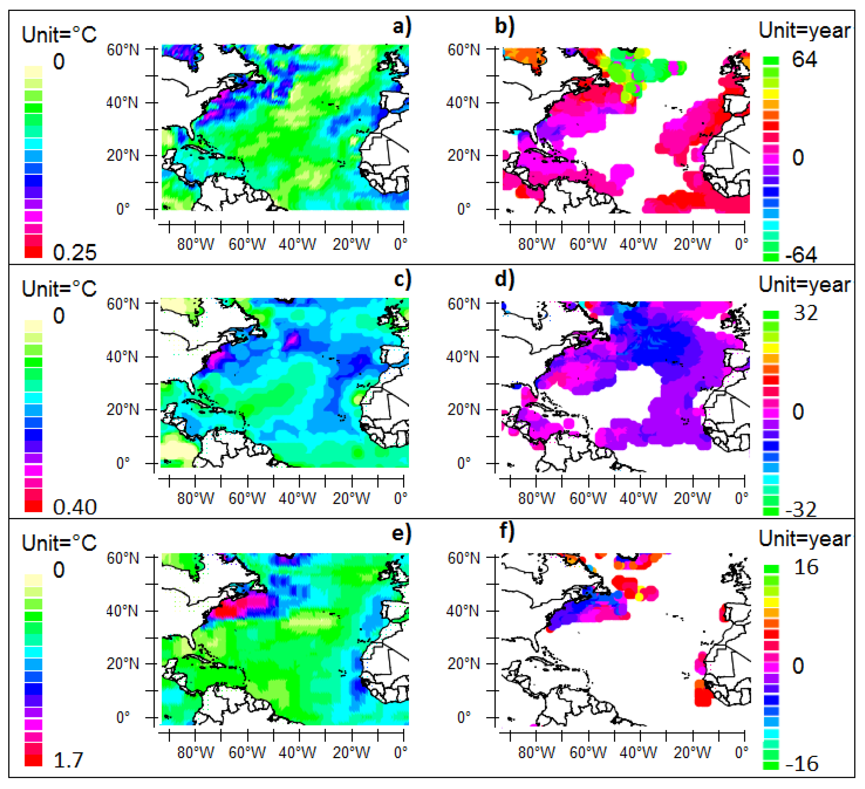
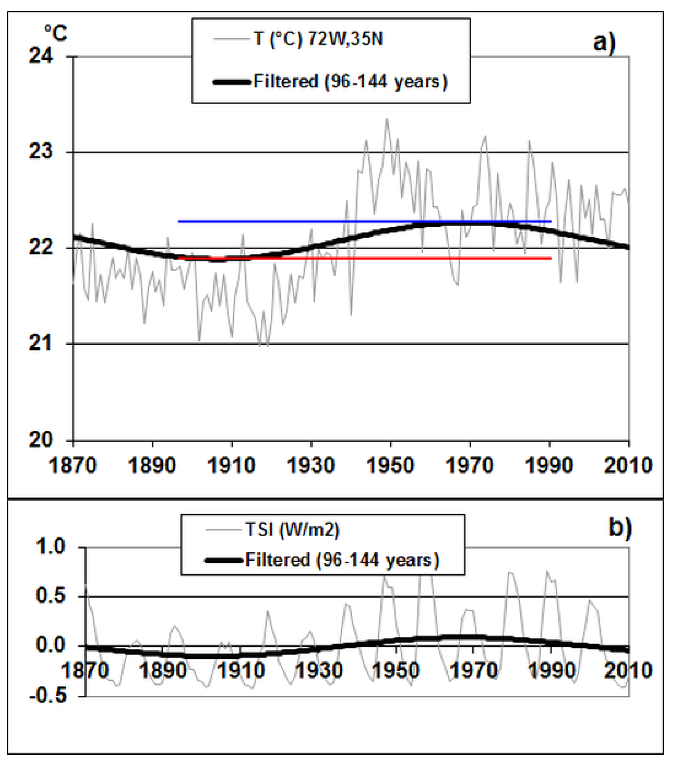
In Figure 2, three periods are represented, 32, 64 and 128 years from the cross-wavelet analysis of SST scale-averaged within the three bands 24–48, 48–96 and 96–144 years, the reference signal being the sunspot number used as a proxy of solar irradiance. More precisely, the cross-wavelet analysis is used to examine the phasing, which reveals the evolution of the amplitude of SST anomalies occurring around the gyre versus the solar irradiance. The upper limit of the last region is constrained by the length of the series. Although the cross-wavelet analysis is scale-averaged within the 96–144 year band close to the length of the observation period, the results are insensitive to edge effects (Figure 3). This exception results from the quasi-periodicity of the data (the SST and the sunspot number) in that band, which is a significant benefit from the continuous Morlet wavelet transforms (the Morlet wavelet operates on a finite time interval unlike the Fourier transform).

The SST anomaly is visible all around the gyre in Figure 2a,b, although its magnitude varies, being nearly in phase with the sunspot number, only slightly delayed in the northern and southern parts of the gyre. The SST anomaly out of the gyre, which reaches 0.10 °C, is in phase opposition with respect to the anomaly around the gyre, which points out the antinode outside the gyre.

In Figure 2c,d the SST anomaly in the 48–96 year band exhibits an annular structure with a quasi-uniform phase concomitant with the solar irradiance. This is not ascertained in the band 24–48 years, as shown in Figure 2e,f: the SST anomaly remains confined from the eastern coast of the Northern America to 50° W in longitude, anticipating the solar irradiance at its northern edge before migrating to the south.

This suggests the absence of resonance around the gyre in the 24–48 year band: the SST anomaly originates where the western boundary current leaves the continent and vanishes where it escapes from the gyre. Therefore the 32-year period GRW is to be considered as a harmonic of longer periods. By contrast, the amplitude and the phase of the cross-wavelet around the gyre exhibit great similarities in the Figure 2a–d, whereas edge effects cannot be suspected in the 48–96 year band.

The concept of GRW, that is, long-period Rossby waves wrapping around sub-tropical gyres, is developed from Figure 2, with this interpretation supported by (1) the spatial structure of the magnitude of SST anomalies in the 96–144 and 48–96 year bands (Figure 2a,b and Figure 2c,d respectively) while this is absent within the 24–48 year band, which suggests a resonant feature of GRWs; (2) the nearly uniformity of the phase of the anomaly around the gyre and (3) the evidence of an anomaly nearly in opposite phase along the North Atlantic Drift mainly visible in Figure 2a,b.

Although SST data are less accurate before 1950, their spatial structure that is observed over the period 1870–2010 in Figure 2a,b shows their consistency throughout the North Atlantic. Indeed, those results require coherence of the data to extract information about long term trends, conditions that are not fulfilled in the South Atlantic and in the other oceans. Coherence of the reconstructed data in the North Atlantic results from both the density of sampling over space and time as well as the reconstruction method developed by the Met Office Hadley Centre to validate those data.

3.2. Subharmonic Mode Locking of Long-Period Gyral Rossby Waves (GRWs)

The modulated geostrophic current being non-divergent in the equations of motion, multiple turns may overlap. This implies that the first baroclinic mode, first radial mode Rossby wavelength has no upper limit. This is because the duration of heating of the mixed layer around the gyre compensates for wave damping due to the Rayleigh friction as the period increases, both being proportional to the period but with antagonistic effects.

The average period of the yearly fundamental GRW is inherited from easterlies that force quasi-stationary waves in tropical oceans, which is to say from the average period of rocking of the intertropical convergence zone. This results from the variation in warm water masses carried by the western boundary currents, which gives rise to the oscillation of the pycnocline depth at mid-latitudes of the gyres [14]. Resulting westward-propagating baroclinic Rossby waves are formed, embedded in the wind-driven current.

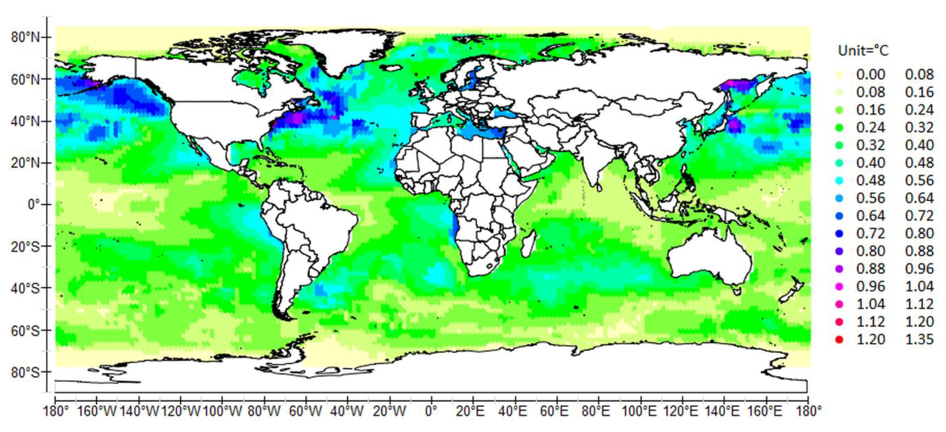
Consider the number of turns corresponding to the period of 128 years close to that of the Gleissberg cycle. The ratio of the estimated apparent half-wavelength of the 128-year period GRW on the circumference of the gyre is (λ/2) × 128/8/circumference where λ/2 is the apparent half-wavelength of the 8-year period GRW, that is, the length of the internal antinode estimated from the cross-wavelet power of the SSH (

Table 1. Subharmonic modes of 128-year period Gyral Rossby Waves (GRWs). λ/2 is the estimated apparent half-wavelength of 8-year period GRWs [14].

	North Atlantic	South Atlantic	North Pacific	South Pacific	South Indian
λ/2 (km)	3400	2700	4900	2300	5500
Mean latitude of the gyre	27.78° N	24.71° S	26.37° N	26.30° S	30.35° S
Circumference of the gyre (km)	16,300	20,800	25,800	25,900	19,400
(λ/2) × 128/8/circumference	3.34	2.08	3.04	1.42	4.54
Probable subharmonic modes	2	2	2	1	3

). It is an upper bound of the number of turns around the gyre (the subharmonic mode). This estimator is biased because of the deceleration of the wind-driven recirculation after the western boundary currents leave the continents so that the internal antinode is stretched and its length is over-valued [14]. However, the subharmonic modes can be identified from the observation of the 64-year period SST anomalies where the western boundary currents leave the continents (Figure 4). The resonance can only occur if the number of turns corresponding to the half-wavelength of the 128-year GRW is even. When this number is odd, the GRW cannot resonate because it cannot wrap entirely around the gyre, which can be highlighted from the SST anomalies that are much contrasted. They show that only the subharmonic modes in the north and South Atlantic and in the North Pacific are even, SST anomalies being at least equal to 0.5 °C whereas no anomaly is visible in the South Pacific and in the South Indian Ocean, which suggests subharmonic modes are odd. This additional information allows us to deduce the most probable subharmonic mode in the five subtropical gyres, that is, 2 in the North and South Atlantic as well as in the North Pacific, 1 in the South Pacific and 3 in the South Indian Ocean. The most questionable value concerns the South Atlantic due to the low amplitude of the resonance, which concerns both the half-wavelength of the 8-year period GRW and the SST anomaly.

3.3. The Solution of the Equations of Motion

3.3.1. Forcing Effects

Contrary to short-period waves, long-period GRWs are no longer produced by a purely remote resonance from equatorial waves whose periods do not exceed 8 years. As shown in Figure 2a,b, SST anomalies observed in the band 96–144 years around the North-Atlantic gyre are indicative of an imbalance between ingoing and outgoing heat fluxes resulting from the circulation of the anti-cyclonic resultant polar current, while surface fluxes are balanced inside and outside the gyre. When SST anomalies are positive, they stimulate transfer of sensible and latent heat to the atmosphere, as well as infrared radiation of the surface whereas those heat fluxes are reduced when anomalies are negative.

Therefore, GRWs are forced from the direct incidence of solar irradiance cycles whose spectrum is spread to higher periods; solar and orbital cycles can exceed several centuries, even hundreds of millennia. To account for this phenomenon, in the equations of motion the forcing terms $X$ and $Y$ which initially represent the surface stress, are zero (there is neither forcing current at the western boundary nor surface stress forcing) and $E$, which initially represents the evaporation rate (forcing on the surface of the ocean), is replaced by $–A.I$ where $I$ is the net heat flux through the ocean-atmosphere interface along the path of the GRW ($A$ is a dimensional constant). The minus sign indicates that the flux is positive when it is outgoing: a negative flux warms sea water, hence the lowering of the thermocline leading to a positive surface height perturbation $\eta$. Therefore, forcing of the Rossby wave results from the variations in solar irradiance in the bandwidth considered for the resonance.

Concerning the ingoing heat flux through the sea surface, the amplitude h* of the oscillation of the thermocline is simply the result of heating of the mixed layer under the effect of variation of the solar irradiance in the characteristic band. It is such that $\frac{h^{*}}{2}=q_{i}t/\left(C_p\rho \mathsf{\Delta }{T}^{*}\right)$ where $q_i$ is the variation in net surface solar radiation, t is the elapsed time, that is, $t=2/\pi \times T_{1/2}$, $T_{1/2}$ being the half-period, $C_p$ the specific heat capacity of sea water considered as constant in the temperature range, equal to 3990 J/Kg/K, $\rho$ is the density of sea water, that is, 1.03 T/m³. The flux $q_i$ is estimated from the net surface solar radiation $Q_i$ by filtering the Total Solar Irradiance (TSI) [20] in the band 96–192 years that frames the 128-year period owing to the subharmonic mode locking which the GRWs are subject: $\mathsf{\Delta }TSI$ = 0.27 W/m², that is, slightly higher than what is obtained in the band 96–144 years (Figure 3). So $q_i=Q_i\mathsf{\Delta }TSI/TSI$ ($Q_i$ = 110 W/m²) at mid-latitudes from [21]. The corresponding value h* is nearly 1.3 m at low and high latitudes. It is only indicative since the real value is much higher because of the amplification process.

3.3.2. Momentum Equations

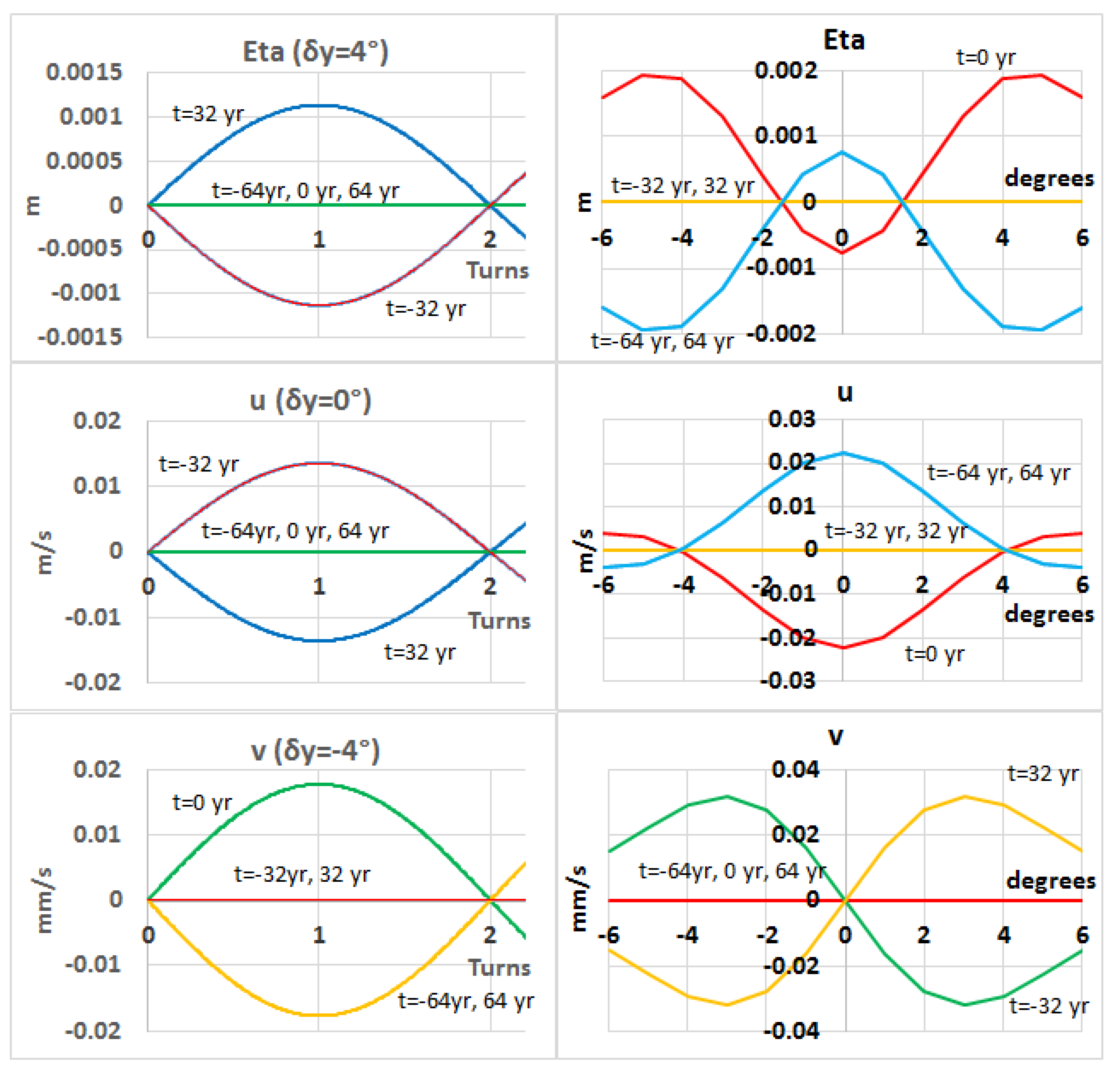
The equations of motion are solved for stationary, boundless waves, taking into account forcing effects all around the gyre. Intensification of the western boundary current being not essential in the overall functioning of the gyre, the western boundary is ignored. The solution of the equations of motion is represented in Figure 5 and Figure 6.

In Figure 5 the forcing term relative to the solar irradiance is a sinusoid ω = 2π/T, T = 128 years and the variation in Total Solar Irradiance (TSI) ∆TSI = 0.27 W/m². The length of partial sums of Fourier series is 1 versus both the longitude and the time. The decay rate of friction r = αω is 2 × 10⁻⁸ s⁻¹ (α = 12.9). The radial current $v$ is in phase with solar irradiance ($v$ is positive outwardly of the gyre), the surface height perturbation $\eta$ is in quadrature with solar irradiance as well as the polar current $u$ ($u$ is positive when it is anti-cyclonic). The positive feedback of the anti-cyclonic polar current on the thermocline depth is not taken into account.

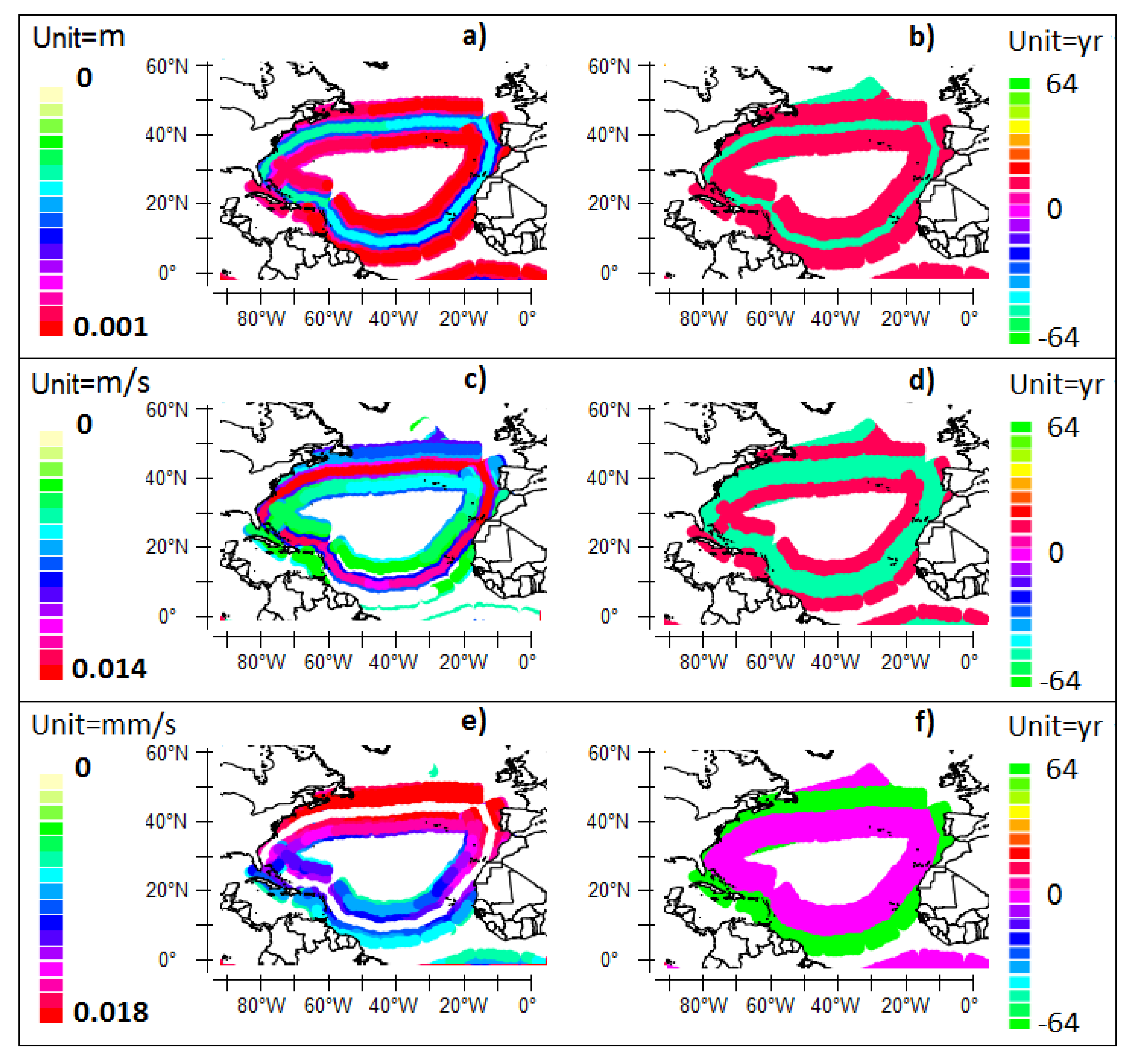
In Figure 6 the wind-driven current velocity is supposed to be 0.038 m/s [14]. The western intensification resulting from the narrowing of the streamlines is ignored. The phase refers to the anti-cyclonic modulated current velocity around the gyre. The antinode around the gyre is in quadrature relative to forcing. Only the phase of a part of the Rossby wave out of the gyre is represented. It bends in the direction of the pole as soon as it leaves the gyre, being in opposite phase relative to the antinode around the gyre. The polar current velocity is in quadrature relative to forcing around the gyre, that is, in phase with the internal antinode (around the gyre). The product $u{H}_1$ of the polar current velocity by the depth of the pycnocline is nearly constant around the gyre. So, the main factor of variation of the polar current velocity $u$ is the pycnocline depth. The radial current velocity is in phase with forcing [22]. Like in Figure 5, the positive feedback of the anti-cyclonic polar current on the thermocline depth is not taken into account.

The radial structure of the internal antinode around the gyre shows a depression along the midline of the gyre flanked by two symmetric bulges in opposite phase compared to the midline (Figure 6a,b). But the central part contributes little to the growing of the antinode that mainly occurs along the two sides. To simplify what is called the internal antinode actually concerns both sides only. Moreover, the central SSH anomaly cannot be guessed from the SST anomaly (Figure 2a), probably due to the viscosity of sea water which is not taken into account in the equations of motion. The solution properly reflects the widening of the gyre resulting from the presence of the two bulges.

The polar current results from the coexistence of currents flowing in the opposite direction (Figure 6c,d), that is, a strong stream that follows the midline of the gyre and two weak peripheral currents. Radial currents converge toward the midline of the gyre or diverge either side (Figure 6e,f).

The radial structure of the internal antinode is different from the meridional structure of equatorial Rossby waves whose first meridional mode exhibits a single bulge symmetrical with respect to the equator. This results from the difference in forcing effects. Solar irradiance, orthogonal to the surface of the ocean, only forces the amplitude of the GRWs whereas in the tropical belt the forcing is exerted both on the amplitude of the waves and on the velocity of modulated geostrophic currents because of surface stress forcing, evaporation during ENSO events [22,23,24] and geostrophic forces at the tropical basin scale.

3.4. Evolution of Gyral Rossby Waves (GRWs)

As concerns 4- and 8-year period resonantly forced waves, the western (internal) and eastern (external) antinodes represent an apparent half-wavelength. Within a period, a warming phase occurs during which warm water is accumulated along the gyre, followed by a cooling phase during which the warm water leaves the gyre. The resonance of GRWs can occur indeed only if an antinode develops outside the gyre, in phase opposition with the antinode around the gyre, as this happens for short periods.

Similar to short-period resonantly forced waves, growth of the internal antinode of long-period resonantly forced waves results from the radial currents that flow in quadrature relative to the antinode. Growth is maximum at the same time as the convergent radial current velocities, half a period before the ridge is formed at the antinode. At this time, the radial currents vanish. On the contrary, deepening of the internal antinode is maximum at the same time as the divergent radial current velocities, half a period before the trough is formed at the antinode. At this time, the radial currents vanish again.

The internal antinode grows during the warming phase. In opposite phase, a trough is formed along the external antinode. The velocity of the polar modulated geostrophic current reaches a maximum while it flows anti-cyclonically, that is, in the same direction as the wind-driven current. The resultant velocity, sum of velocities of modulated geostrophic and steady wind-driven polar currents, peaks. At this time, the velocity of the external modulated geostrophic current reaches a maximum, while flowing in the reverse direction. Being the sum of the external modulated geostrophic and steady wind-driven currents the resultant North Atlantic Drift slows down or vanishes. Thus, warm water accumulates around the gyres, transfers from internal to external antinodes being locked. Half a cycle later, a trough is formed at the internal antinode and a ridge at the external antinode. The polar currents vanish or reverse, being the superposition of two currents propagating in the opposite direction. Conversely, the external modulated geostrophic currents flow poleward and the resultant current that is the sum of the modulated geostrophic current and the steady wind-driven current flowing in the same direction peaks. At this stage, the internal antinode is weakly or not fed while warm water is advected from this antinode to the external antinode. The same transfer method applies to GRWs of different frequencies. Consequently, the resonance of GRWs leads to the formation of a poleward propagating mixed layer represented by the successive warm water masses advected to half a wavelength during half a cycle whatever the frequency.

The functional analysis of antinodes as well as polar and radial modulated geostrophic current velocities clearly appears from the solution of the equations of motion. But this apparent simplicity reflects the fact that sea water is supposed inviscid. Actually, the resonance of GRWs is much more difficult to decipher from observations because of the viscosity which smooths the radial structure of the internal antinode and the polar current, as a result of bottom and lateral friction. Modelling is however essential to understanding the underlying mechanisms.

The solar and orbital forcing efficiency with zero wind stress results from the imbalance between incoming and outgoing fluxes. In the absence of resonance of GRWs the ingoing flux is balanced mainly by evaporation. On the other hand, downwelling resulting from the convergence of radial currents while the intensity of forcing is peaking makes the GRW behave as a heat sink, immersion of the heated surface layers reducing evaporative processes. In contrast upwelling induced by the divergence of radial currents while the intensity of forcing is minimum makes that the GRW acts as a heat source, by sustaining evaporative processes. The imbalance is maximized when forcing reaches an extremum. It is all the larger as the magnitude of the oscillation of the thermocline is greater.

3.5. Positive Feedback Loop of the Polar Current on the Thermocline Depth

Ingoing heat fluxes are issuing through the sea surface as a result of short wavelength radiations, from the western boundary current when the flow rate is increasing in the presence of a temperature gradient between low and high latitudes of the gyre and from the radial currents while they are converging to the gyre. Outgoing heat fluxes result from the long wavelength radiative flux, the latent heat flux and the sensitive heat flux through the sea surface, from the western boundary current when the flow rate is decreasing and from the radial currents while they are diverging from the gyre.

Due to the temperature gradient between low and high latitudes of the gyre, an amplifying phenomenon occurs as the resultant polar current accelerates while flowing anti-cyclonically, when the thermocline is lowering. More heat being transferred from the equator to the poles via the western boundary currents the thermocline lowers more at high latitudes and modulated geostrophic currents accelerate further. It results from Figure 6c,d that this positive feedback of the anti-cyclonic polar current on the thermocline depth occurs during the half period that precedes the maximum of forcing. However, the SST anomaly that reflects this positive feedback is nearly in phase with forcing as shown in Figure 2a,b, which means the polar current continues to accelerate until forcing peaks, concomitantly with the deepening of the thermocline. Owing to the positive feedback loop, the maximum polar current velocity occurs while it flows anti-cyclonically, when growth of the internal antinode is maximum.

The recirculation of the polar current around the gyres cools the North/South Equatorial Currents, all the more as upwelling is stimulated by accelerating eastern boundary currents due to tightening of the current lines leading to vertical pumping effects, that is, the Canary Current in the North Atlantic, the Benguela Current in the South Atlantic, the West Australian Current in the South Indian Ocean, the California Current in the North Pacific and the Peru (Humboldt) Current in the South Pacific. Thus, despite the upsurge due to this positive feedback, the amplitude of oscillation of the thermocline and the flow of modulated geostrophic currents remain tightly controlled while not changing the potential vorticity of the eastern boundary current significantly. Furthermore, the amplification is limited by the ability of sea water to warm up at low latitudes and by the bottom friction of the modulated geostrophic currents.

The efficiency of the positive feedback loop is enhanced as the temperature lowers at high latitudes of the gyre. This may occur when the polar front advances, increasing the temperature gradient between low and high latitudes. This has the effect of increasing the speed of the polar current, therefore the amount of warm water transported towards the poles, which induces the retreat of the polar pack. This negative feedback may have had a significant role in the long term control of climate.

The GRW strengthens the horizontal pumping effect on the western boundary current evidenced by the anti-cyclonic modulated polar current that results from the conjugation of the modulated geostrophic current and the steady wind-driven current. As already seen in short waves [14], this pumping effect causes an increase of the total volume transported by the western boundary current and the abrupt change in the potential vorticity of the western boundary current as soon as it is forced to leave the coast while flowing at the critical latitude for which the phase velocity of the cyclonic GRWs is lower than the speed of the anti-cyclonic wind-driven recirculation. Indeed, subtropical gyres cannot be completed with a purely inertial boundary layer because fluid leaving the boundary layer would retain the potential vorticity it had acquired in lower latitudes and so would not match that of the interior flow. More generally, when surface forcing terms are introduced in the linear equations of an inviscid ocean, a Sverdrup balance is achieved in the entire ocean except the western boundary layer, where a steady state cannot be reached unless additional effects come into play, a way to circumvent these issues [15].

Consequently, the GRWs play a key role in the adjustment of geostrophic forces around and outside the gyre to high latitudes, completing the current models (barotropic and baroclinic) in the presence of transient geostrophic eddies. Owing to the positive feedback loop, the modulated response of subtropical gyres raises considerable interest since it opens up a new field to be investigated: long-period baroclinic waves appear to be involved in total volume transport and abrupt change in potential vorticity of western boundary currents.

3.6. Adjustment of the Gyre to Maintain Resonance Conditions

As occurs for shorter wavelengths, the resonance determines geostrophic forces throughout the basin and takes precedence over the non-resonant phenomena whose impact is less. Resonant phenomena absorb maximum solar energy as the wave and forcing are synchronized. Otherwise, during its evolution the wave is necessarily in phase opposition with forcing and therefore its amplitude is less. Maintaining resonance conditions may involve accurate adjustments when the forcing period differs slightly from the natural period of subharmonics, all the more as the bandwidth of forcing cycles is narrow. The fitting parameters are the average latitude of the gyres and their circumference (a decrease in the average latitude of 0.1°, that is, 11.1 km, generates an increase in the circumference of the gyre of the North Atlantic of 122 km). Therefore, under the effect of forcing, regulation phenomena may occur to maintain the conditions of resonance despite changes in the period of the oscillations of solar irradiance.

3.7. The Atlantic Multidecadal Oscillation (AMO)

The AMO signal is usually defined from the patterns of SST variability in the North Atlantic once any linear trend has been removed. In models, AMO-like variability is associated with small changes in the North Atlantic branch of the Thermohaline Circulation [25] although historical oceanic observations are not sufficient to associate the derived AMO index to present-day circulation anomalies.

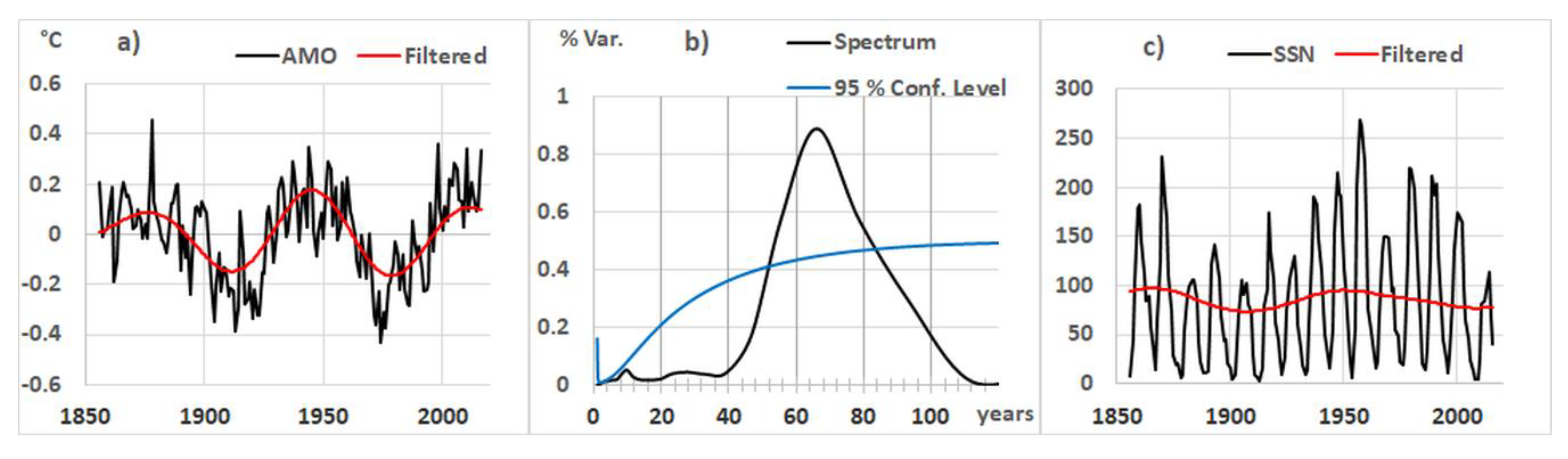
In the conceptual framework of this work, the AMO must be related to the resonance of 64-years average period GRWs. The Fourier power spectrum of the AMO confirms this deduction (Figure 7b): the maximum is reached at nearly 64 years. On the other hand, the AMO is almost in phase with the Sun Spot Number (SSN) as shown if Figure 7a,c. The amplitude of the cross-wavelet of the AMO, considering the SSN as the reference signal, is 0.083 °C and the phase is 3.2 years only. The amplitude is low in the context of the Figure 7a because the AMO is the result of an integration of SST over a large area.

3.8. A Quasi-Isolated Thermodynamic System

Not only does the resonance of the GRWs produce a powerful geostrophic current superimposed on the wind-driven recirculation, which explains the modulation of the subtropical gyres as well as that of the drift currents but it opens a new way to study the long-term climate variability. This is based on the fact that the subtropical gyres alter thermal exchanges between the oceans and the atmosphere. This is particularly true at mid-latitudes while the gyre behaves like a heat source or, on the contrary, a heat sink. Those thermal transfers result from the modification of the vertical temperature gradient of sea water, which enhances or, on the contrary, lessens convection processes.

To quantify the energy transfer from the oceans to the continents resulting from the perturbation ΔT of the SST at high latitudes of the gyres, the unperturbed state of the system has to be considered at first, which implies that the average energy captured by the earth is completely re-emitted in space. This supposes that the energy transfers are averaged over one or even several years to remove fingerprints of transient phenomena that cause an imbalance in energy budget during the annual cycle: anthropogenic effects being ignored, this is the case, for example, of the formation of sea ice during the winter followed by its melting during the summer.

The perturbed state of the system tends to a new steady state in which a new thermal equilibrium occurs between the oceans and the continents. The impact on climate resulting from the perturbation ΔT of the SST at high latitudes, which either stimulates or, on the contrary, reduces evaporation, is substantial because it generates baroclinic instabilities that may lead to the formation of cyclonic or, on the contrary, anti-cyclonic systems of the atmosphere. Carried by the jet streams those synoptic atmospheric instabilities provide heat exchange between the oceans and continents. This exchange, based essentially on the evaporation/condensation processes, is rapid. It occurs from specific SST anomalies, which are located on the gyres at mid-latitudes, to particular inland regions [26,27]. The remote impact of SST anomalies on inland areas has been demonstrated using the oscillation in the 5–10 year band of both SST anomalies and precipitation as a marker of condensation.

The perturbed state of the system behaves like a quasi-isolated thermodynamic system because thermal exchanges are mainly ruled by evaporative processes. This implies that the heat accumulated in the gyre at mid-latitudes is conserved on a planetary scale. Indeed, outgoing heat fluxes through the sea surface are the differential fluxes resulting from the perturbation ΔT of the SST at high latitudes of the gyres. Those differential fluxes are threefold: the radiative flux $q_r$, the latent heat flux $q_l$ and the sensitive heat flux $q_s$ (see Appendix A for details of the differential fluxes deduced from the SST anomaly). Knowing the radiative flux $Q_r$, the latent heat flux $Q_l$ and the sensitive heat flux $Q_s$ of the unperturbed state of the system, the differential fluxes are calculated so that $q=\mathrm{d}Q/\mathrm{d}T.∆T$. As shown in

Table 2. Expression of the mean heat fluxes resulting from the SST anomaly ΔT at high latitudes of the gyres. $Q_r$ is the outgoing radiation flux, $Q_l$ the latent heat flux, $Q_s$ the sensible heat flux, from “European Reanalysis ERA40” [21]. The differential fluxes $q_r$, $q_l$ and $q_s$ are induced by the SST anomaly. The sensitive heat flux is approximate (Appendix A: The differential fluxes deduced from the SST anomaly). The SST and the ∆T are indicative since they are intended for the comparative study of fluxes.

SST °C	ΔT °C	${\mathit{Q}}_{\mathit{r}}$ W/m2	${\mathit{q}}_{\mathit{r}}$ W/m2	${\mathit{Q}}_{\mathit{l}}$ W/m2	${\mathit{q}}_{\mathit{l}}$ W/m2	${\mathit{Q}}_{\mathit{s}}$ W/m2	${\mathit{q}}_{\mathit{s}}$ W/m2
12	0.14	−45	−0.09	−50	−0.46	−15	−0.30

, the latent heat flux $q_l$ is by far the largest since it is −0.46 W/m² at high latitudes of the gyres, whereas the radiative flux is −0.09 W/m²: this outgoing flux is negligible in comparison to the conservative flux $q_l+q_s\approx -0.76$ W/m². This flux is indeed considered conservative in the context of this study because the thermal exchanges between the oceans and the continents are fast in comparison with the periods of GRWs [26,27] so that outgoing radiative fluxes can be neglected during heat exchanges.

In the thermally quasi-isolated perturbed state of the system, heat exchanges occur until a new thermal equilibrium is reached. Due to the large heat capacity of seawater relative to the continents, the perturbation ΔT of the SST is not altered significantly during heat transfer between the gyres and the impacted inland areas. The persistence of the perturbation ΔT mainly reflects the circulation of the polar current, which leads to the renewal of the mixed layer at high latitudes of the gyres while maintaining the vertical temperature gradient.

Then, more global processes take over to warm or cool the continents globally as a result of the long-period of the perturbation ΔT. Consequently, everything happens as if the perturbed state was deduced from the unperturbed state by equalizing the perturbation ΔT of the SST at high latitudes of the gyres and the resulting perturbation of the land surface temperature.

3.9. The Resonance of Gyral Rossby Waves (GRWs) during the Holocene

From what has been seen, the resonant character of the subtropical gyres should be observed in the climate variability, the global temperature anomaly deduced from ice core archives being supposed to be roughly equal to the SST anomalies on the gyres at mid-latitudes. ¹⁸O obtained from Greenland Summit Ice Cores GISP2 (Greenland Ice Sheet Project 2 Ice Core [26]) are used as proxies of land-ocean temperature in the northern Atlantic. ¹⁸O data are calibrated considering a variation of 0.67‰ ¹⁸O/°C [28,29]. On the other hand, the Total Solar Irradiance (TSI) is obtained from ¹⁰Be and ¹⁴C stored in polar ice cores and tree rings [20].

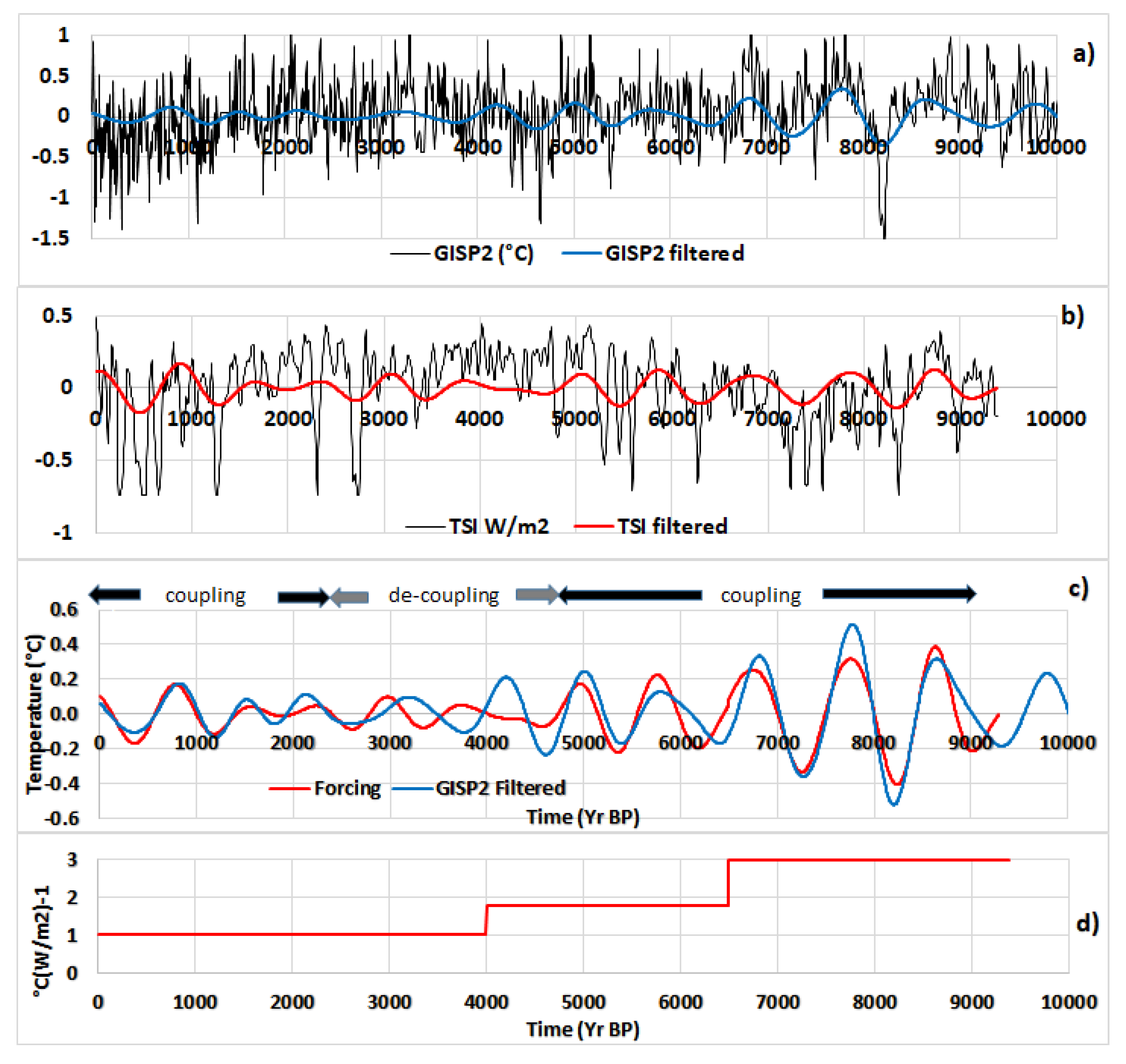
In the North Atlantic, the Figure 8c displays similarities between the TSI multiplied by the forcing efficiency and the global temperature into the band 576–1152 years characteristic of the 64 × 12 = 64 × 3 × 2² = 768 year period whose subharmonic mode is 3 × 2² (number of turns made during half a period). The two curves show a similarity mainly over the interval covering 9000 to 6000 years BP, that is, when the forcing efficiency is maximum.

The forcing efficiency (Figure 8d), that is, the sensitivity of the global temperature (°C) to the solar insolation (W/m²), varies over time: equal to 3.0 °C × (W/m²)⁻¹ between 9000 and 6500 years BP, it decreases to 1.0 °C × (W/m²)⁻¹ after 5000 years BP. This is because the response of the gyre to the variations in the TSI is all the more enhanced as the gradient of the sea water temperature between low and high latitudes of the gyre is steeper. At the beginning of the Holocene, the pack ice extended further south, which explains the high radiative forcing efficiency. Then, gradual withdrawal of the pack ice made the positive feedback of the polar current on the thermocline depth less efficient.

Between 5000 and 2500 years BP the amplitude of solar irradiance into the band 576–1152 years decreases (Figure 8b) and the GRW disassociates from the solar irradiance cycle, both the amplitude and period. During this period of decoupling the GRW does not weaken because of the remanence of geostrophic forces throughout the gyre and along the drift currents but its period lengthens, which indicates that the centroid of the gyre drifts poleward. The GRW is coupled to the solar cycle again between 2500 years BP and present during the upsurge of the solar cycle. Therefore, the resonance of the 3 × 2² subharmonic mode GRW appears to be the main driver of climate variability during the Holocene.

3.10. The Resonance of Gyral Rossby Waves (GRWs) during Glacial-Interglacial

The association of climate variability to orbital forcing, that is, the precession, the obliquity and the eccentricity, emphasizes the resonant character of long-term climate variability. On one hand the impact of orbital variations on climate is not proportional to the amplitude of solar irradiance variations. On the other hand, over the past 800,000 years, the period of oscillation of glacial—interglacial that dominates is 100,000 years, showing it is mainly subject to eccentricity. During the interval from 3.0 to 0.8 million years before our era, the period of 41,000 years prevailed, corresponding to changes in the obliquity of the Earth, what is named the transition problem.

To explain how orbital forcing controls the climate system, Davis and Brewer [12,13] investigated a forcing based on the latitudinal insolation gradient, which is dominated by both obliquity (in summer) and precession (in winter). According to them, the insolation gradient acts on the climate system through differential solar heating, which creates the Earth latitudinal temperature gradient that drives the atmospheric and ocean circulation, precursor of what is exposed here.

The observations suggest that a resonance phenomenon occurs, filtering out some frequencies in favour of others. This hypothesis, issued for several decades, has so far not found plausible physical basis. This suggests a priori that the resonance of GRWs is the missing link to solve this riddle. Effectively, there exists a coupling between orbital forcing and the amplitude of the GRWs. But, contrary to what occurs during the Holocene, the narrow frequency bands of orbital forcing make the latter much more selective.

To tune the natural frequency of GRWs to the forcing frequency while keeping the subharmonic mode, the latitude of the centroid of the gyres has to be shifted as a result of Eqution (6). Since several subharmonic mode GRWs coexist, the tuning of the natural periods to the forcing periods requires the mean latitude ${\phi }_0$ of the gyres oscillates around the central value.

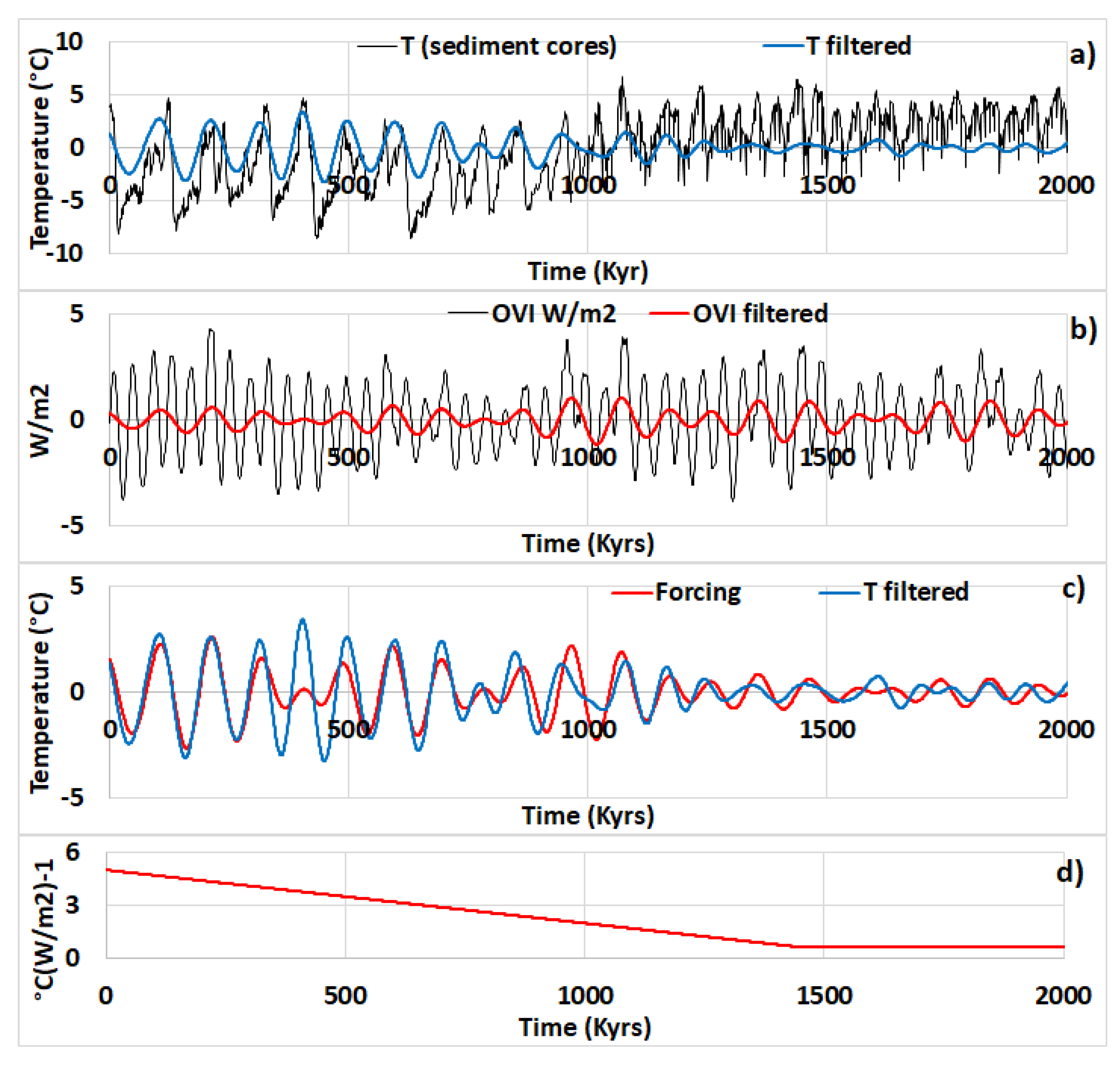
Sediment core records [30] allows us to elucidate what occurred 0.8 M yrs ago when the period of the global mean temperature skipped from 41 to 100 K yrs. Indeed, when the temperature is calibrated relative to ice core records, the sediment records can be used in a quantitative manner over the period 0 to 2 M yrs BP during which processes of diffusion that tend to blur the proxy used for the estimation of temperature changes, that is, ^δ18O in foraminifera, can be neglected (Figure 9 and Figure 10).

Sediment core records show that the orbital forcing efficiency increases as concerns eccentricity (Figure 9d) whereas it is subject to rapid variations for the obliquity (Figure 10d). The former increases linearly from 0.7 to 5.0 °C × (W/m²)⁻¹ since 1425 Krs BP. Although the evolution of the period of eccentricity can hardly be detected accurately from the wavelet analysis, which widens the frequency band of series obtained by Berger, 1992 [31], it can be inferred that it is connected to the period of forcing approaching the natural period of GRWs, that is, 98.3 K yrs. Tuning between orbital forcing and GRWs appears to be extremely sharp due to the narrowness of the frequency band of eccentricity (

Table 3. The periods of forcing compared to the natural periods of Gyral Rossby Waves (GRWs) and the shifting of the average latitude of the centroids resulting from the tuning. Subharmonic modes in the South Pacific have to be divided by 2. In the South Indian Ocean, they have to be multiplied by 3/2.

Orbital Parameter	Period of Forcing (K yrs)	Period of Resonance (K yrs)	Subharmonic Mode in the Atlantic	Shifting in Latitude	Direction
Precession	23.5	24.6	3 × 27	40′	southward
Obliquity	41	49.2	3 × 28	2°30′	southward
Eccentricity	100	98.3	3 × 29	15′	northward
Eccentricity	360	393.2	3 × 211	1°15′	southward

).

The coupling relaxes between 450 and 350 K yrs BP when the forcing collapses and then recovers when the amplitude of the forcing increases again. During this time interval, the stability of the oscillation of the GRW, which continues even when the forcing vanishes owing to the remanence of large-scale geostrophic forces, suggests it is the fundamental wave, that is, the GRW whose amplitude is directly subject to the influence of orbital forcing. The increase in forcing efficiency reflects that the period of orbital forcing and the natural period of GRWs become closer over time (Table 3 and Figure 9d). Indeed, the successive advance and retreat of the polar front cannot be invoked to explain the sudden changes in the amplitude of the GRWs because the dynamics of the polar pack is much faster than what is observed here, from what we have seen during the Holocene: a few thousand years versus nearly 50 K yrs.

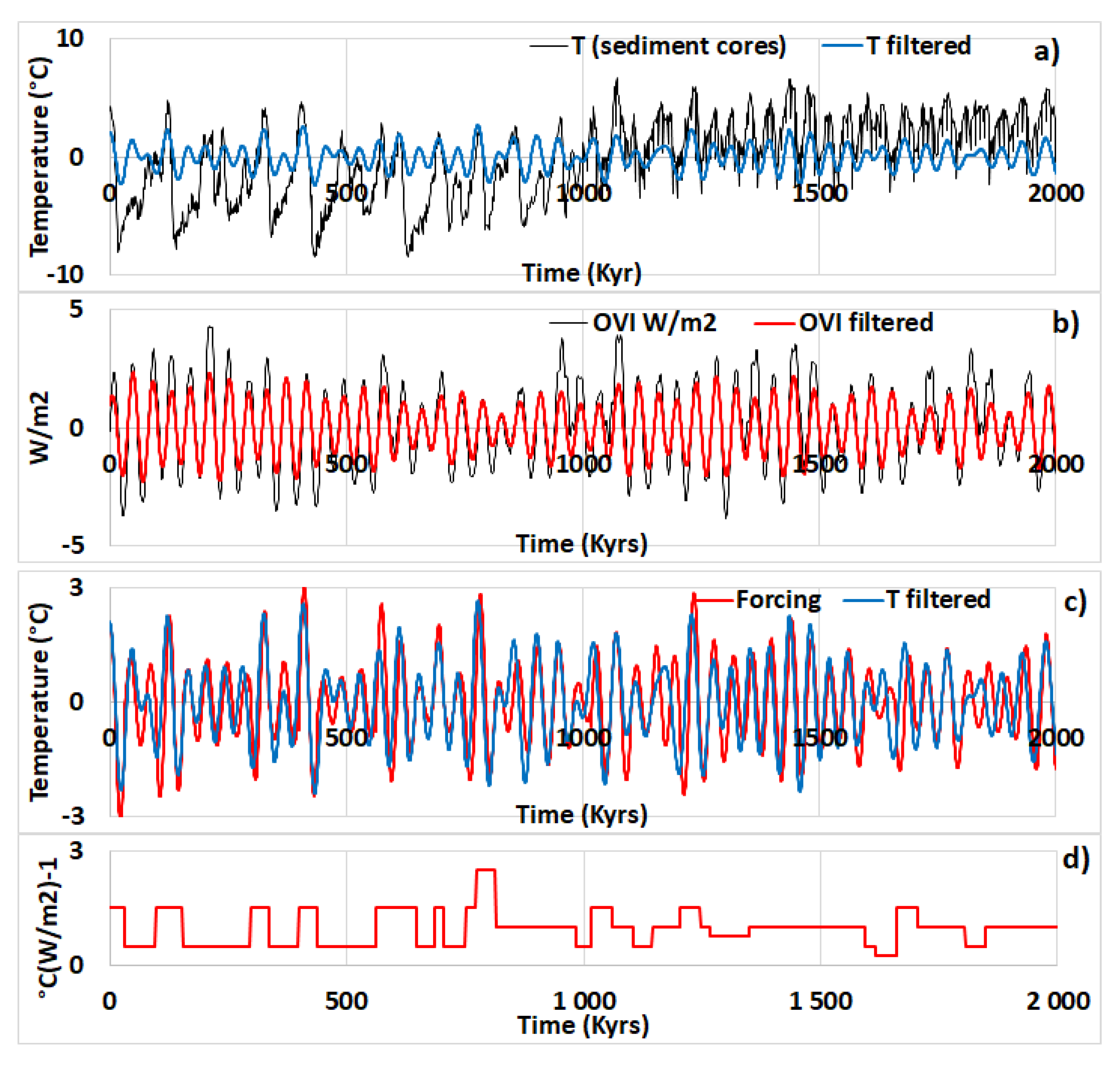
As concerns obliquity, the mean forcing efficiency does not change significantly over the time interval considered, around 1 °C × (W/m²)⁻¹ but the stability of the coupling is better before 0.8 M yrs BP, the efficiency remaining close to 1 °C × (W/m²)⁻¹ during half of the time while it oscillates between 0.5 and 1.5 °C × (W/m²)⁻¹ between 0.8 M yrs BP and present. This seems to confirm that these instabilities result from the coupling between the two subharmonics of GRWs whose natural frequencies are 49.2 and 98.3 K yrs (Table 3), disturbances decreasing with the amplitude of the component of 98.3 K yr period. It should be noticed a significant increase in forcing efficiency 0.8 M yrs ago, that is, when both subharmonics have nearly the same amplitude. On the other hand, the mean forcing efficiency related to obliquity remains low in comparison with that of eccentricity, due to the difference in forcing and natural periods.

Consequently, the transition problem can be explained simply from the variation in the forcing efficiency of the eccentricity. Beyond 0.8 million years, the drift of the period of eccentricity shows that the subharmonic mode of the fundamental wave goes from 3 × 2⁹ to 3 × 2⁸, that is, the forcing period is ruled by the obliquity by means of a 2°30′ shift of the latitude southward. Such a transition should have been accompanied by significant modifications of the geostrophic forces in both hemispheres due to a drastic reduction in the number of turns made by the fundamental GRWs.

4. Summary

To summarize the main properties of GRWs:

• Cyclonic non-dispersive GRWs resonantly forced by solar and orbital variations with zero wind stress require their phase velocity is lower than the speed of the anticyclonic wind-driven current in which they are embedded, at the critical latitude where the western boundary current leaves the continent to enter the subtropical gyre. The speeds of the modulated geostrophic polar and radial currents are proportional to h, that is, the magnitude of the oscillation of the thermocline that results from the first baroclinic mode, first radial mode Rossby waves around the gyres.
• The oscillation of the thermocline is subject to a positive feedback loop in which the effects of a small disturbance induces an increase in the magnitude of the oscillation. This is because the acceleration of the polar current enhances the warming of the western boundary current that transfers more rapidly warm water from low to high latitudes. Thus, an amplification occurs, limited by the ability of sea water to warm up at low latitudes and by cooling resulting from upwelling along the eastern boundary currents of the gyres.
• Multi-frequency GRWs are superimposed. Sharing the same polar currents, they are coupled. Consequently, a subharmonic mode locking occurs, which means that the average periods of GRWs are deduced by recurrence, the period of order n being a multiple of the period of order n − 1. Therefore, GRWs are characterized by a number of revolutions, that is, their subharmonic mode, which corresponds to half their apparent wavelength.
• When the period of GRWs increases, the Rayleigh friction is offset by the increase in the duration of heating of the mixed layer so that the amplitude of GRWs does not vanish. This remarkable property enables the GRWs to be tuned to forcing over very long periods as is the case for orbital variations of the Earth, without mitigation.
• The efficiency of the positive feedback loop is enhanced as the temperature lowers at high latitudes of the gyre, which strongly depends on the location of the front of the polar pack.
• Resonant forcing of GRWs requires the natural frequencies have the ability to be finely tuned to the frequencies of solar and orbital forcing by shifting the centroid of the gyres along a meridian. Several natural periods of GRWs may be tuned to different forcing periods when they are sufficiently close.

Thus, the interest aroused by the modulated responses of subtropical gyres, which has been ignored so far while being supported both by the observations and the theory, is promising in physical oceanography (the total volume transport of western boundary currents, their abrupt change in potential vorticity at critical latitudes, the global ocean circulation) and long and very long-term climate variability while complementing the current theories.