Article

Integration of the CEL and ML Methods for Landing Safety Prediction and Optimization of Full-Scale Track Design in a Deep-Sea Mining Vehicle

1
First Institute of Oceanography, Ministry of Natural Resources, Qingdao 266061, China
2
National Deep Sea Base Management Center, Qingdao 266237, China
3
China Offshore Oil Engineering Corp CNOOC Ltd., Tianjin 300461, China
4
Shandong Provincial Key Laboratory of Marine Environment and Geological Engineering, Ocean University of China, Qingdao 266100, China
5
Sanya Oceanographic Institution, Ocean University of China, Sanya 572024, China
6
Department of Civil, Environmental and Geomatic Engineering, University College London, London WC1E 6BT, UK
7
Department of Engineering, University of Cambridge, Cambridge CB2 1PZ, UK
*
Authors to whom correspondence should be addressed.
J. Mar. Sci. Eng. 2025, 13(8), 1584; https://doi.org/10.3390/jmse13081584
Submission received: 22 July 2025 / Revised: 14 August 2025 / Accepted: 16 August 2025 / Published: 19 August 2025

Abstract

Ensuring the safe landing of deep-sea mining vehicles (DSMVs) on soft seabed sediments is critical for the stability and operational reliability of subsea mineral extraction. However, deep-sea sediments, particularly in polymetallic nodule regions, are characterized by low shear strength, high compressibility, and rate-dependent behavior, posing significant challenges for full-scale experimental investigation and predictive modeling. To address these limitations, this study develops a high-fidelity finite element simulation framework based on the Coupled Eulerian–Lagrangian (CEL) method to model the landing and penetration process of full-scale DSMVs under various geotechnical conditions. To overcome the high computational cost of FEM simulations, a data-driven surrogate model using the random forest algorithm is constructed to predict the normalized penetration depth based on key soil and operational parameters. The proposed hybrid FEM–ML approach enables efficient multiparameter analysis and provides actionable insights into the complex soil–structure interactions involved in DSMV landings. This methodology offers a practical foundation for engineering design, safety assessment, and descent planning in deep-sea mining operations.

1. Introduction

With the expansion of marine resource exploration into deep-sea territories, the demand for specialized underwater mining systems has increased globally [1,2,3,4]. Among these, deep-sea mining vehicles (DSMVs) play a pivotal role in harvesting valuable seabed minerals such as polymetallic nodules and sulfides [5,6,7,8]. However, their deployment is hindered by the unique mechanical traits of deep-sea sediments, namely, their low resistance to shear, high compressibility, and near-fluid behavior, all of which pose challenges for vehicle stability and control [9,10]. Understanding the settlement behavior of DSMVs on these sediments is critical to ensure their operational stability and minimize their impact on sensitive marine environment. Tracked mining vehicles (as shown in Figure 1) have emerged as the most viable solution for these applications because of their ability to distribute loads and maintain mobility across soft, yielding substrates [11,12]. Therefore, the settlement mechanism of tracked mining vehicles in deep-sea sediments has received increasing attention.
The traction and settlement behavior of tracked DSMVs are intrinsically linked, especially under conditions involving significant soil deformation [13]. The classical pressure–sinkage relationship proposed by Bekker remains a foundational framework for understanding terrain interactions, particularly highlighting how soil cohesion, fraction, and saturation levels influence deformation behavior [13,14,15]. Nevertheless, its applicability is often limited under the large-deformation and low-strength scenarios typical in deep-sea environments [16,17], and seabed soil heterogeneity presents challenges for these models. Variations in sediment properties complicate predictions, as noted in studies on seabed heterogeneity [18,19,20]. Research on DSMV ground interactions has historically been constrained by the difficulty of recreating authentic deep-sea conditions in laboratory settings. The unique mechanical behavior of abyssal soils—particularly their rate-dependent and strain-softening responses—renders traditional experimental methodologies inadequate [4,21,22,23,24,25]. Moreover, the complexity and scale of full-track systems further complicate physical replication, thereby necessitating advanced computational methods that can simulate realistic seabed interactions under varying environmental and operational parameters. Prior work by Einav and Randolph [26] emphasized the significance of strain-softening behavior in large-deformation problems, highlighting the necessity of incorporating more advanced constitutive formulations in such contexts.
Although widely adopted in terramechanics, Bekker’s model exhibits limitations when applied to highly heterogeneous and viscoelastic deep-sea sediments [15,16], prompting the need for more nuanced numerical approaches in extreme geotechnical conditions. Numerical simulations, particularly finite element method (FEM), have emerged as a powerful tools for addressing these challenges. Early work by Benson [27] laid the foundation for CEL-based FEM techniques applied to problems involving extreme deformation and contact separation, providing critical support for their adoption in geotechnical applications. Unlike traditional experimental approaches, FEM allows for the detailed modeling of complex geotechnical phenomena, such as large deformations, sediment–fluid interactions, and the dynamic response of sediments under loading [28,29,30,31,32]. Janarthanan & Kuttikrishnan [33] examined the sinkage behavior of deep-sea soil under mining vehicle operations using numerical simulations and experimental studies, emphasizing the importance of optimizing the design configuration to ensure stability under varying soil conditions. Amudha et al. [34] analyzed breakout and sinkage forces of tracked vehicles on soft marine clays using finite element methods and field-calibrated models, further supporting the need for integrated predictive approaches in seabed mobility assessments. More recently, Janarthanan et al. [35] performed multi-body dynamic simulations to compare inline and offset track configurations for DSMVs, revealing how geometric layout influences traction efficiency and sinkage in soft seabed conditions. Sun et al. [36,37] investigated the sinking pattern of a single track plate under different conditions with the Coupled Eulerian–Lagrangian (CEL) method, indicating the necessity of considering different track parameters and soil mechanical parameters. Luan et al. [38] analyzed the dynamic stresses generated in the seabed by moving deep-sea mining vehicles, highlighting the critical influence of seabed properties and vehicle parameters on the stress distribution using numerical case studies. Xia et al. [39] developed a multibody dynamics model for a four-track deep-sea mining vehicle and simulated its straight-line motion, demonstrating the impact of vehicle dynamics and seabed conditions on travel performance and stability. Liu et al. [40] investigated the bearing capacity of consolidated clay subjected to track loads from deep-sea mining vehicles, stressing the importance of soil consolidation and stress distribution patterns for assessing vehicle-induced deformation. Similar approaches have also been explored internationally. Tho et al. [41] applied a three-dimensional Eulerian finite element method to simulate penetration of spudcans into seabed soils, successfully capturing large soil deformations and validating the approach against centrifuge tests. Agarwal et al. [17] analyzed wheel–granular media interactions using the Material Point Method (MPM) and Resistive Force Theory (RFT), providing insights into wheel/track–soil dynamics relevant to deep-sea vehicles. Gonzalez and Iagnemma [42] employed deep learning techniques to estimate terrain slip and classify terrain types for ground vehicles, illustrating the potential of ML for terrain–vehicle interaction prediction, while Chavez-Garcia et al. [43] demonstrated that convolutional neural networks trained on simulated terrains can robustly predict ground traversability, reinforcing the strategy of using simulated datasets to inform ML-based safety or mobility models. Zhang et al. [44] studied soil failure patterns caused by vehicle motion trajectories to evaluate the traction performance of deep-sea mining vehicles. Zande et al. [45] applied a coupled numerical–experimental framework to examine track–soil interaction for planetary rovers, offering insights relevant to DSMV track design. White and Randolph [46] investigated seabed–structure interaction using strain-softening models to predict penetration resistance under cyclic loading.
However, most existing studies have focused on simplified track geometries or small-scale models, neglecting the critical influences of full-scale DSMV operations. Moreover, the mechanical behavior of deep-sea soft sediments is often approximated using basic constitutive models, which fail to capture key factors such as strain softening and rate dependency. Several recent studies have demonstrated that finite element software combined with modified constitutive soil models can be employed to characterize this property of deep-sea sediments more accurately. Xiao et al. [47] studied the effects of strain softening on the penetration resistance of offshore bucket foundations in nonhomogeneous clay, emphasizing the importance of accounting for soil heterogeneity and strain-softening mechanisms in design and analysis. Xie et al. [48] developed a convenient method for simulating large-deformation submarine landslides, highlighting the need to incorporate shear-softening and strain rate correlation effects for accurate numerical predictions. Guo et al. [49] conducted a comprehensive study on the bearing capacity factors of T-bar penetrometers during penetration into deep-sea sediments, providing valuable insights into the soil resistance characteristics under various penetration stages. Their findings underscore the necessity of considering the complex soil behavior and penetration dynamics in deep-sea environments.
Although these methods enhance the fidelity of modeling full-scale DSMV subsidence under soft seabed conditions, simulating the entire track system remains a nontrivial task because of its intricate structural and mechanical interdependencies. For instance, Kim and Hossain [19] developed numerical strategies for anchor and soil interaction under strain-rate-dependent seabed conditions, which provide useful parallels for DSMV–seabed interaction analysis. The complexity arises from the interplay between multiple factors, including track–soil contact mechanics, the geometric and material properties of the undercarriage, and the effects of transient dynamic loads during operation. Consequently, such simulations demand considerable computational resources and processing time. To address these limitations, recent research has increasingly explored predictive modeling techniques and algorithmic optimization strategies that aim to reduce the computational burden without compromising model integrity. Among these, machine learning (ML) has gained significant traction in geomechanics and engineering applications [50,51,52], owing to its ability to learn nonlinear relationships and adapt across various data domains [50,51,52,53,54,55]. Ensemble-based frameworks such as random forest (RF) have shown strong potential for improving predictive robustness. By integrating the outputs of numerous base learners, these models enhance both accuracy and generalizability under diverse conditions [56,57,58]. The RF algorithm constructs a collection of decision trees trained on different subsets of the data and combines their predictions to form a consensus output [59]. Its simplicity of deployment, versatility across different input feature spaces, and resilience to irregular data distributions make it a valuable tool for engineering prediction tasks [60].
To address the challenges associated with predicting the landing behavior of DSMVs on ultra-soft seabed sediments, this study establishes a hybrid computational framework that integrates a CEL finite element model with an ensemble-based machine learning algorithm. The proposed FEM model incorporates an improved strain-softening and rate-dependent constitutive law to simulate the full-scale dynamic track–seabed interaction under various sediment strengths, sensitivity levels, and loading conditions. The quantitative influence of these parameters on the dimensionless settlement depth is systematically analyzed, and the underlying mechanisms are discussed. To overcome the high computational cost of large-deformation FEM analyses and enable efficient prediction, the simulation outputs are further used to train a RF regression model. This multiparameter prediction approach achieves high accuracy while offering greater generalizability than conventional empirical formulas.
This study contributes a dual-method evaluation framework that combines high-fidelity numerical simulation with data-driven learning for DSMV landing safety assessment. The framework not only enhances predictive capability in soft marine geology but also provides practical insights for the structural design and operational planning of DSMVs in complex deep-sea environments.

2. FEM Method for Obtaining the DSMV Sinking Process

2.1. CEL Numerical Method

To effectively represent the substantial deformation and material flow that occurs when vehicles interact with the seabed, this research adopts the CEL method [27]. By integrating Eulerian meshes that remain stationary with Lagrangian meshes that move with the material, CEL is capable of accurately simulating the severe distortions typical of soft seafloor environments and scenarios often beyond the reach of traditional modeling approaches [61]. In the ABAQUS 2022 (Dassault Systèmes, Waltham, MA, USA) software framework, this hybrid strategy assigns Eulerian treatment to regions undergoing extreme deformation, whereas relatively stable zones are handled through Lagrangian modeling. A volume fraction tool facilitates the representation of material distribution by generating a field where the Eulerian volume fraction (EVF) varies between 0 and 1, indicating the presence of materials. Figure 2 illustrates the comparative behavior of the two methods. The system ensures accurate tracking of material flow through remeshing procedures and adheres to conservation laws, whereas dynamic interaction at the Eulerian–Lagrangian boundaries (where EVF equals 1) is managed via contact mechanics. CEL is extensively utilized in explicit dynamic simulations, including scenarios such as track–terrain interactions, making it a robust approach for handling complex deformation and contact phenomena.

2.2. A Constitutive Soil Model That Integrates Strain Softening and Strain Rates

To realistically represent the mechanical behavior of soft deep-sea soils, this study adopts a strain-softening and rate-sensitive constitutive model, which was originally proposed by Einav and Randolph [26]. This model enables a dynamic update of the undrained shear strength based on the cumulative plastic strain and applied shear strain rate. Under undrained conditions, soft seabed soils exhibit post-peak stress–strain softening, quantified by the cumulative plastic strain [26,62]. Under compression by an applied load, strain rate effects increase the soil’s undrained shear strength [63,64,65,66,67]. These effects can be expressed using semilogarithmic or power-law functions [68,69,70,71].
S u = S u 0 α β = S u 0 δ r e m + 1 δ r e m exp 3 ξ / ξ 95 1 + η γ . / γ r e f . n
where Su is the current undrained strength and Su0 is the undrained shear strength of the undisturbed soil. δrem is the inverse of the soil sensitivity St, denoting the ratio between the fully remolded and initial shear strengths; ξ95 is the accumulated shear strain when 95% soil strength degradation occurs between the intact and fully remolded conditions; accumulated absolute plastic shear strain, ξ; η is the viscosity coefficient; where n is the shear-thinning index; γ · ref is the reference shear strain rate; and γ · is shear strain rate. Each increment (dt) with respective to γ · in Equation (2) can be calculated from
γ . = Δ ε 1 Δ ε 3 Δ t
The process of realizing the modified constitutive soil model through numerical modeling is as follows: Shear strength is initially defined by Su0 and updated dynamically using cumulative strain and rate effects through the VUSDFLD and VGETVRM subroutines [47,48]. The shear strength evolves iteratively, as calculated from the cumulative plastic strains and updated coefficients (α and β), enabling the precise simulation of soil deformation under dynamic loading.
To assess the feasibility of the proposed model and verify its simulation accuracy, a falling cone test previously reported in the literature was numerically reproduced. The experimental setup was conducted under atmospheric pressure conditions and is widely used in geotechnical laboratories to estimate soil shear strength based on penetration depth. The geometrical parameters of the simulation model were based on a falling cone apparatus manufactured by GEONOR Inc., Oslo, Norway, as shown in Figure 3a. In the test, the cone tip contacted the soil surface and was released from a magnetic holder, with shear strength calculated using Hansbo’s empirical equation [72]. Although the original falling cone test was performed in air under atmospheric conditions, the soil sample used was saturated clay. Therefore, in the corresponding numerical simulation, the soil density was adjusted to its submerged density by subtracting the density of water. This buoyant unit weight assumption is commonly employed in marine geotechnical modeling to simulate soil behavior under effective stress conditions. Accordingly, the revised simulation more realistically captures the large-deformation behavior of saturated cohesive soils while remaining consistent with the reference experimental setup.
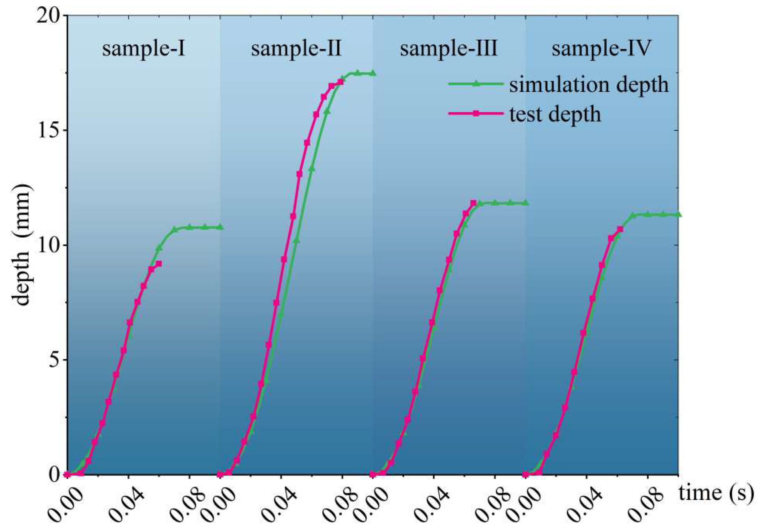
Table 1 lists the soil sample parameters. A 100 g cone with a 30° tip angle was used in the simulation. As shown in Figure 4, the numerical simulation results show good agreement with the experimental data, indicating that the CEL-based numerical model combined with a modified soil constitutive model is capable of capturing the large-deformation behavior during dynamic penetration. This validation, although conducted under simplified conditions, lays the groundwork for the subsequent application of the model to simulate DSMV–seabed interaction under submerged conditions.

2.3. Numerical Model of the Track–Soil Sinkage Interaction

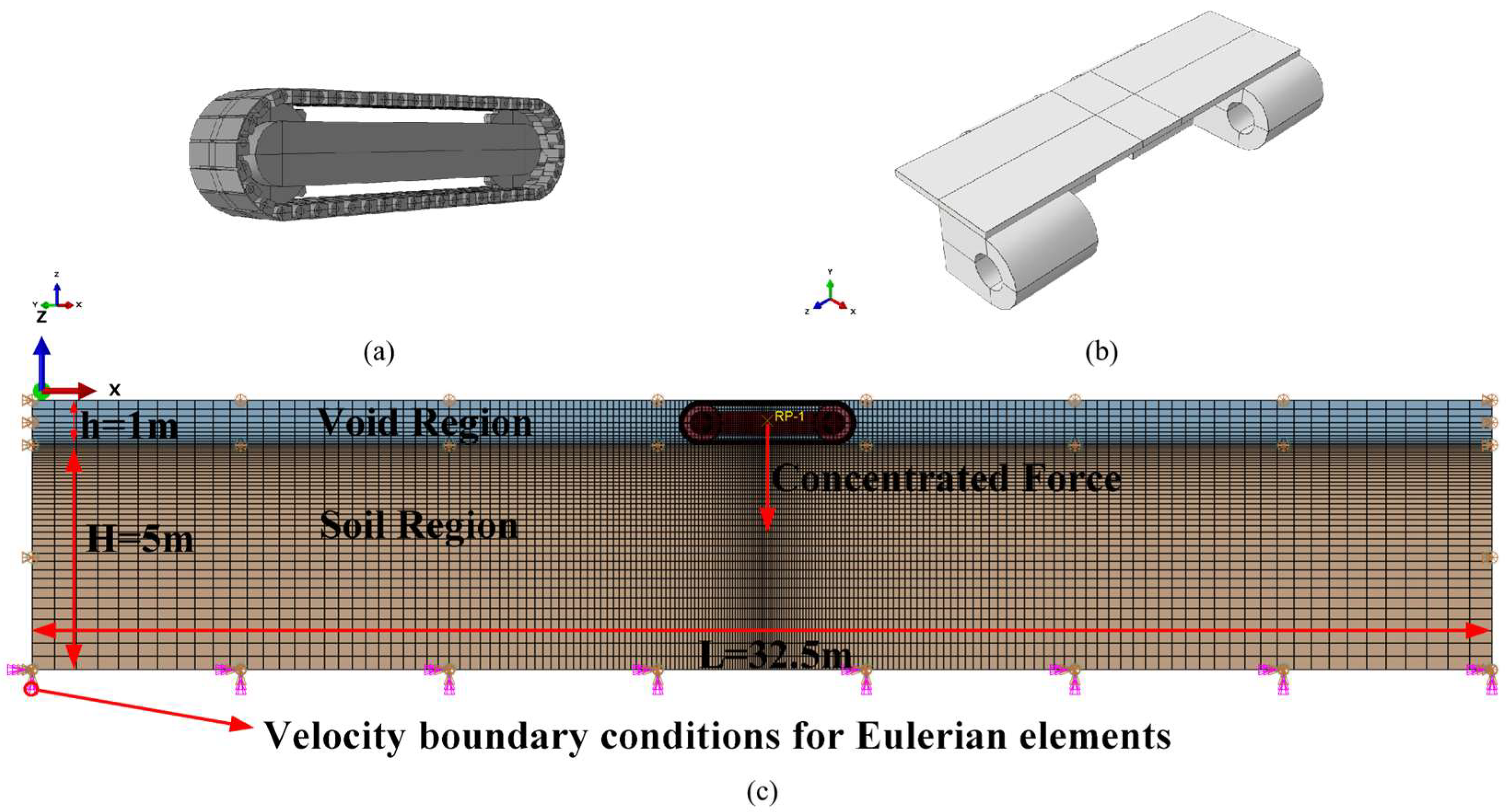
The full-scale track–soil interaction model developed in this study is inspired by the “Pioneering-I” DSMV prototype designed by Sun et al. [36]. The track system modeled includes detailed mechanical components such as single-pin plates, sprockets, and support assemblies. Figure 5a shows a gear radius of 0.5 m and a spacing of 3.12 m between gears. The single-pin track plate design (Figure 5b) has dimensions of 0.6 m × 0.15 m × 0.01 m.
The seabed model, constructed with Eulerian elements, consists of material and void regions to simulate sediment displacement and ensure convergence. Figure 5c shows the parameters: the soil height is five times the track height, with the length and width scaled to 10 and 20 times the track size, respectively. The void region is 1 m high. To approximate the submerged conditions typical of deep-sea environments, the soil material was assigned a buoyant density, obtained by subtracting the density of seawater from the total soil density. This assumption enables the simulation to reflect effective stress conditions and is commonly used in marine geotechnical modeling. Owing to sediment softness, the track is modeled as a rigid body with constraints applied at its center of mass for velocity and load control.
Separate Eulerian and Lagrangian meshes are used for the simulation. The C3D8R and EC3D8R elements model the Lagrangian and Eulerian regions, respectively, providing accurate representations of seabed–track interactions. This validated framework ensures reliable analysis of DSMV operations in deep-sea environments.

2.4. Sensitivity Analyses of Mesh Parameters

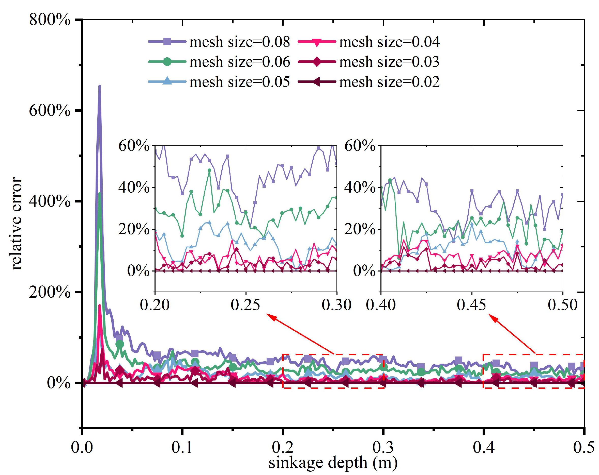
To ensure numerical stability and computational efficiency, a mesh sensitivity analysis was conducted on the Eulerian domain, with the mesh division information detailed in Table 2. First, the sediment resistance acting on the DSMV was tested under different mesh sizes for the same sinking depth. The relative errors between models with different mesh sizes were subsequently calculated, and the results are shown in Figure 6, with the simulations performed on a 12th Gen Intel(R) Core(TM) i7-12700 CPU. Overall, the calculation results with mesh sizes of 0.05 m, 0.04 m, and 0.03 m have relatively good convergence. Within certain depth ranges, the results for the 0.05 m mesh size exhibited larger deviations than those for the 0.03 m and 0.04 m mesh sizes. In contrast, the models with mesh sizes of 0.03 m and 0.04 m maintained better consistency with the 0.02 m mesh model across all depth ranges. This consistency indicates that the model achieves a high level of accuracy at these mesh resolutions, making 0.03 m and 0.04 m suitable choices for balancing computational efficiency and accuracy. This agreement indicates that the model maintains a high simulation accuracy at these mesh resolutions. Considering both the accuracy of numerical convergence and the need for computational efficiency, this study selects a central mesh size of 0.04 m for the densest Eulerian elements. Beyond the core region, the mesh size is gradually increased toward the periphery, with the largest elements reaching 0.5 m at the boundaries. This hierarchical mesh design balances precision in critical areas with reduced computational costs in less critical regions, ensuring an efficient and reliable simulation framework.

3. Results and Discussion

This section provides an analytical discussion of the sinking behavior of the DSMV in deep-sea soft sediments, dividing the analysis into three parts using the proposed numerical model. The first part focuses on the undrained shear strength of the sediment, including its magnitude and spatial distribution. The second section examines the influence of strain-softening and strain rate parameters on the mechanical response of sediment. Finally, the discussion addresses the dynamic factors of the DSMV, such as its weight, bottom velocity, and size of the contact area.

3.1. Effect of the Sediment Undrained Shear Strength

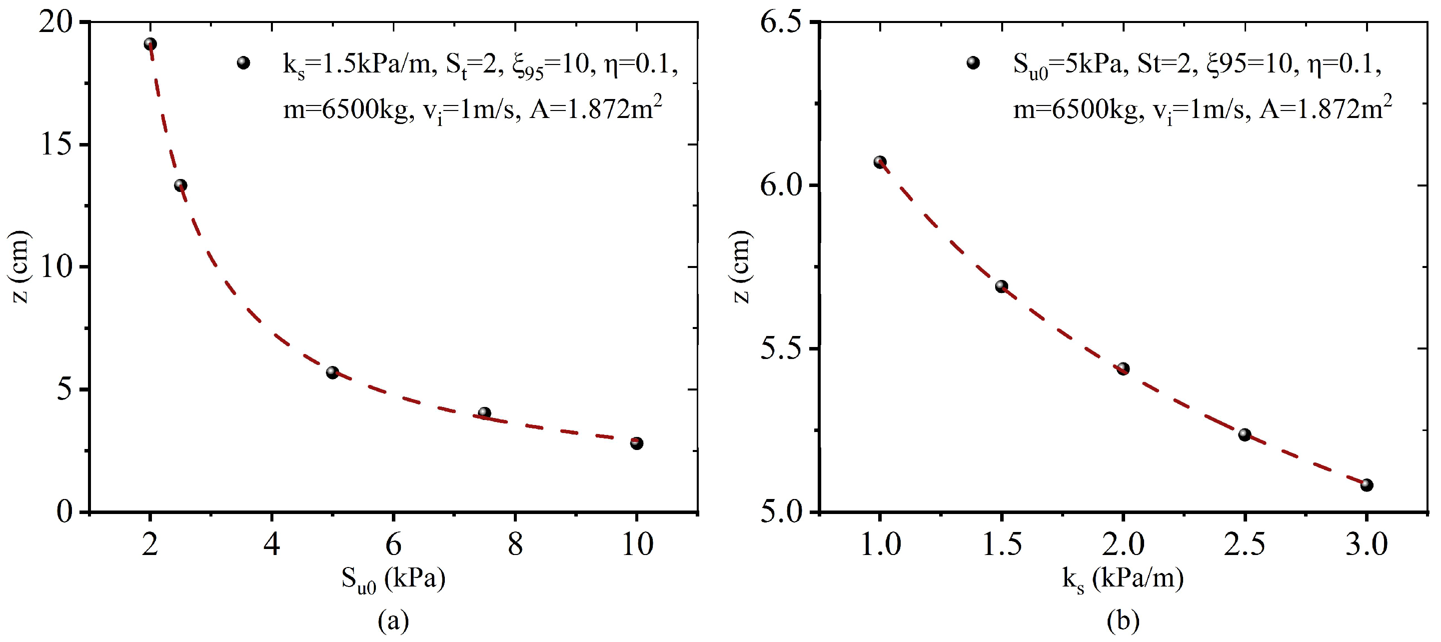
To analyze the effect of the undrained shear strength of the sediment on the maximum sinkage depth, Figure 7a shows the sediment surface shear strength Su0 and its rate of change with depth as a function of the sinkage depth. Under the same softening effect parameter and DSMV dynamic parameter conditions, the maximum sinkage depth of the DSMV exhibits the opposite trend with respect to the sediment surface shear strength, i.e., the maximum sinkage depth of the DSMV decreases with increasing sediment shear strength. The rate of change of the curve decreases as the shear strength increases. The difference in sinking depth is close to 20 cm for the five strength conditions under these conditions. Figure 7b shows the relationship between the maximum sinking depth and the rate of change of shear strength with depth for a shear strength of 5 kPa. Under the same surface shear strength condition, the higher the rate of change in shear strength, the greater the shear strength at the same depth, resulting in a smaller sinking depth of the DSMV. In conclusion, the figure showed that the inverse proportional functional relationship is reflected between the shear strength and the maximum sinkage depth, which is consistent with the relationship described in Equation (3).
This trend reflects the fundamental role of shear strength in resisting local failure. A higher undrained shear strength enhances the mobilized bearing capacity, leading to a more stable stress distribution beneath the track. As the stress path approaches failure, lower shear strength sediments mobilize plastic strain earlier, resulting in deeper penetration. As shown in Figure 8, the cumulative shear strain occurring in the smaller deposits of ks under the action of the tracks is greater, and the shear zone is deeper.

3.2. Effect of the Softening Effect Parameter

To further investigate the influence of softening-related parameters on the settlement behavior of the DSMV, we conducted a parametric study focusing on the soil sensitivity (St), strain at 95% strength degradation (ξ95), and viscosity coefficient (η). These parameters reflect the post-yield strength degradation, softening evolution rate, and sediment resistance to deformation under shear loading, respectively.
As shown in Figure 9a, increasing the soil sensitivity results in a greater maximum sinkage depth. This can be attributed to the reduced post-disturbance shear strength in highly sensitive sediments. Once disturbed, such soils rapidly lose their strength, leading to localized failure zones that facilitate deeper track penetration. The rate of increase in settlement tends to diminish as St continues to increase, indicating a nonlinear sensitivity–sinkage relationship, possibly due to the saturation of strain localization effects. Figure 9b illustrates the effect of ξ95. A higher ξ95 implies that the sediment undergoes more cumulative strain before reaching significant strength degradation. This delays the formation of shear bands, thus improving the load-bearing capacity and reducing settlement. In contrast, lower ξ95 values lead to rapid strength loss and early onset of localized failure. In Figure 9c, the role of viscosity is evident. Sediments with higher viscosity coefficients exhibit a more pronounced resistance to flow, thereby restricting the plastic deformation of soil particles. This dampens the velocity-induced inertial effects during landing and limits the formation of failure surfaces, resulting in reduced sinkage. Figure 10 visually confirms this mechanism, with the higher viscosity leading to a broader strain-hardened region within the sediment below the track, where an increase in shear strength occurs.
These results highlight the critical role of softening characteristics in shaping the post-yield behavior of soil and the transition from elastic-plastic to viscoplastic deformation modes.

3.3. Effect of the Dynamic Parameter Situation

The dynamic conditions of the DSMV, particularly bottom velocity, track–sediment contact area, and vehicle mass, significantly affect its interaction with deep-sea sediments. Figure 11 presents the relationship between these parameters and the corresponding maximum sinkage depth.
The observed trends indicate that higher landing velocities and larger vehicle masses result in increased settlement depths. This is due to the kinetic energy transferred to the soil upon contact, which increases the shear strain rate and accelerates the deformation process. The additional energy input not only induces localized failure but also expands the plastically deformed region beneath the track, as evidenced by Figure 12, which shows the soil velocity field contours. These contours reveal high-velocity zones around the failure fronts, indicating fluid-like flow behavior in low-viscosity sediment.
Conversely, an increase in the track contact area leads to a reduction in pressure applied per unit area, thereby limiting the stress concentration and delaying failure initiation. The stress is more evenly distributed, reducing the severity of plastic deformation and resulting in shallower penetration depths. Among all the dynamic parameters, the bottom velocity has the most pronounced effect on settlement, underscoring the importance of controlling the descent speed during vehicle deployment to avoid excessive embedment.

3.4. Interplay Between Strain-Softening and Rate Effects

The combined influence of strain-softening and rate effects introduces a complex, competing dynamic that governs the overall sinkage behavior of DSMVs. While strain softening reduces the mobilized shear strength with progressive deformation, strain rate effects can lead to transient hardening, enhancing soil resistance under rapid loading conditions. The numerical results illustrate this interplay: at low bottom velocities, strain rate effects are minimal, allowing softening to dominate. In this regime, the shear strength rapidly decreases once yielding begins, resulting in early shear band formation and deep penetration. However, as the landing velocity increases, the rate-dependent hardening partially offsets the softening-induced strength loss, delaying localization and reducing settlement compared with the softening-only case. This antagonistic relationship is further complicated by sediment viscosity. In high-viscosity sediments, the mobilized strength is preserved for longer durations, reducing the softening effects even under slow loading. In contrast, low-viscosity sediments facilitate flow and strength degradation, making the rate effect insufficient to prevent deep penetration even under rapid descent.
Therefore, the final sinkage depth reflects the net outcome of this interaction: the balance between the rate-enhanced stiffness and the degradation-driven weakening. A clear understanding of this coupled mechanism is essential for the optimal design of DSMV landing strategies in heterogeneous deep-sea environments. While the FEM simulations provide detailed insights, they are computationally intensive. To overcome this limitation and support rapid assessments, we developed a data-driven surrogate model using the random forest algorithm, trained on the numerical results.

4. Prediction Model Using the Random Forest Algorithm

4.1. Random Forest Approach

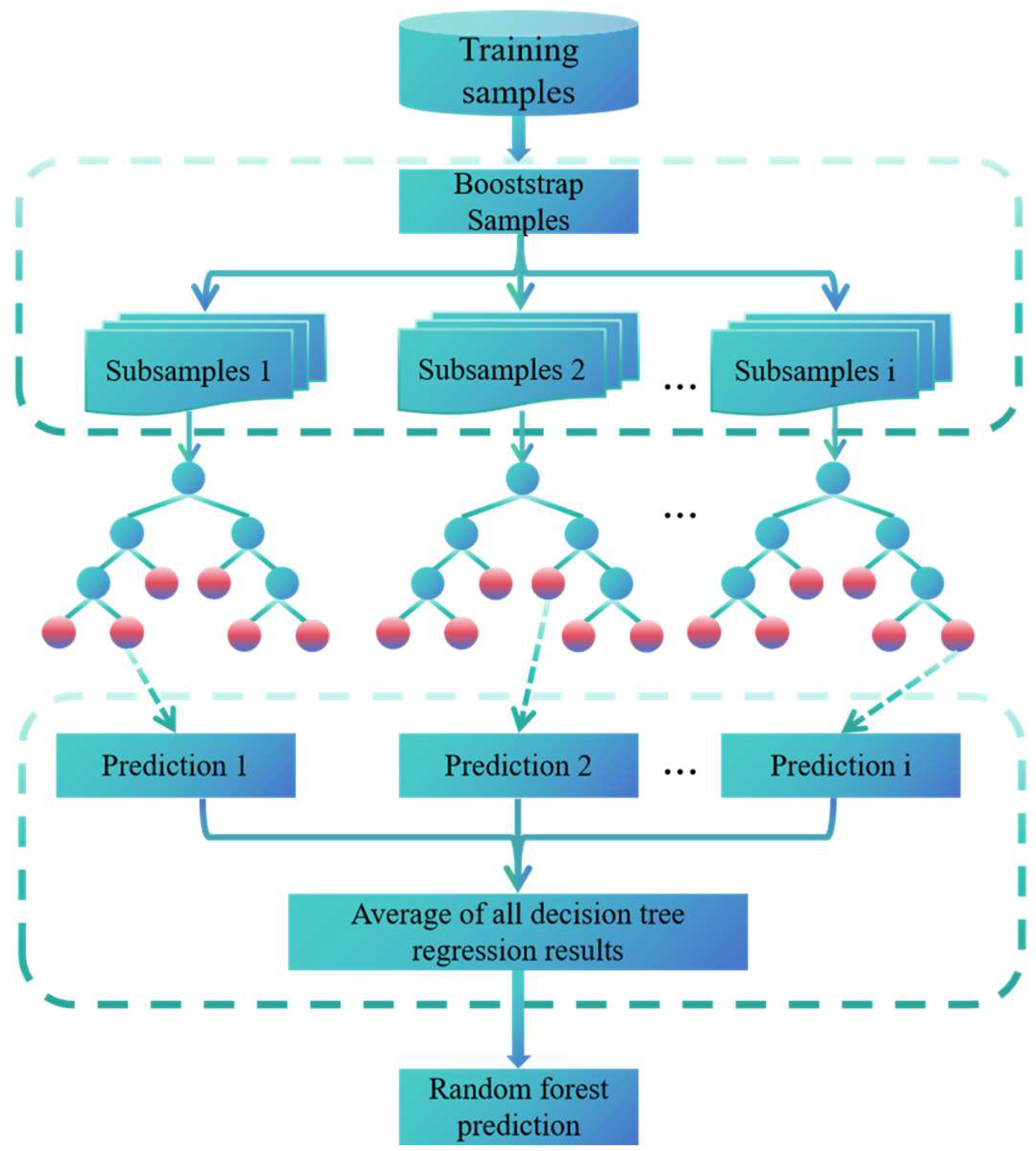
Given the nonlinear and multivariable nature of the DSMV settlement behavior, a random forest regression model is adopted. Random forest is a typical ensemble machine learning model [59], which aggregates the outputs of multiple base models constructed on the dataset to produce a final prediction. This algorithm is well-known for its relative simplicity, its efficiency in handling large-scale datasets, and its ability to maintain predictive accuracy even when the data distribution exhibits significant variability [60]. This ensemble approach builds multiple decision trees and integrates their predictions to capture complex patterns within the high-dimensional input space, thus enhancing robustness and generalization, as depicted in Figure 13. The overall prediction of the random forest is derived by averaging the results of all decision trees in the model [52].
In a random forest model, the construction of individual decision trees adheres to a methodical and iterative framework. Each training set is defined as D = {(x1, y1), (x2, y2), …, (xN, yN)}, where each sample xi comprises n features representing the independent input variables and N denotes the number of training instances. At each node of the decision tree, the algorithm performs recursive data segmentation, dividing the input space into two distinct partitions, R1 and R2, based on candidate feature thresholds. To determine the most effective splitting criterion, all the variables and their potential values are evaluated exhaustively. This iterative assessment mechanism enables the construction of an ensemble where each decision tree captures unique patterns, thereby enhancing the overall accuracy and generalization capacity of the model.

4.2. Dimensionless Sinkage Depth

Machine learning requires a certain number of features (i.e., attributes) to train a model. One of the main challenges is determining the correct number and type of such features from the attributes of a given dataset [73]. The machine learning process generally applies the available feature values directly for model training. This approach makes the process vulnerable to overfitting, prediction errors, bias, and poor generalizability. The key to improving the accuracy and fit of ML is to determine the best set (i.e., grouping) of the correct set of features to best match the feature values. In this paper, we propose a new approach to enhance the feature engineering and selection optimization process for DSMV sinking.
To develop the RF input structure, a dimensionless representation of the sinkage depth is adopted. This method builds upon the traditional energy approach [74]. The total energy Etotal is defined as the sum of the total kinetic and potential energies, and then the soil strength slope ks and the anchor projection equivalent diameter Dp are normalized to obtain the empirical model equation for predicting the penetration z / D p E t o t a l k s D p 4 1 / 3 . The improvement lies in the incorporation of strain-softening and strain rate effects, which play a significant role in characterizing the mechanical behavior of soft sediments. These enhancements enable a more accurate representation of sediment deformation under dynamic loading conditions. The improved energy method is further employed for feature selection and feature engineering, serving as a critical preprocessing step for data preparation in the DSMV predictive model. This comprehensive feature formulation enables the RF model to capture complex coupled influences in a compact, interpretable input format, enhancing both predictive accuracy and training convergence.
Using this finite element model, the maximum sinking depth of the unloaded DSMV(z) can be determined under varying conditions of undrained shear strength, strain-softening parameters, and track dynamic factors. The sum of the kinetic energy when the DSMV hits the seabed and the potential energy at the cessation of motion is defined as the total energy Etotal, and is dimensionless for Etotal and z by setting E t o t a l A B S u 0 + k s z and z / A . Furthermore, the strain rate, strain-softening effect, and soil strength inhomogeneity are considered. The improved empirical formula is defined by Equation (3):
z / A = f δ r e m , ξ 95 , η , E t o t a l A B ( S u 0 + k s z ) = f δ r e m , ξ 95 , η , 1 2 m v i 2 + m g z A B ( S u 0 + k s z )
where m is the wet weight of the DSMV, vi is the initial bottom velocity, A is the contact area of the track, and B is the track width.
In this study, the binary tree-based machine learning integration method, i.e., random forest, is used to predict ( z / A ) . The process of model building consists of the following main steps.
(I) Data definition and generation: The initial step involves identifying the key input features (δrem, ξ95, η, 1 2 m v i 2 + m g z A B ( S u 0 + k z ) ) alongside the predicted output variable ( z / A ) . These output targets are derived from high-fidelity numerical simulations, supplemented by an improved energy-based analytical approach.
(II) Data inspection and partitioning: Preliminary data exploration was carried out to detect potential anomalies and understand variable distributions. Next, the dataset was randomly partitioned into a training subset (90%) and a testing subset (10%) to ensure reliable model development and performance validation.
(III) Model training and hyperparameter optimization: The training subset was employed to fit the random forest regression model. A comprehensive grid search strategy was implemented to fine-tune critical hyperparameters—such as tree count, depth, and minimum split size—based on internal validation metrics, with the goal of maximizing predictive performance.
(IV) Model validation and robustness analysis: To assess model accuracy, standard regression metrics (e.g., R2, MAE, and RMSE) were computed using the test subset. Additionally, K-fold cross-validation and repeated Monte Carlo simulations were conducted to evaluate the model’s generalization capacity and resilience across multiple randomized data splits.

4.3. Establishment of the Prediction Model

In step (I), the model input parameters include δrem, ξ95, η, and Etotal. The output parameter is z / A . Based on the strain parameter characteristics of the DSMV ‘Pioneering-I’ by Shanghai Jiaotong University [36] and a typical deep-sea polymetallic nodule belt [68,69], Table 3 shows a summary of the statistical characteristics of the 257 samples. In step (II), to facilitate more efficient feature selection [75,76], we subsequently performed correlation analyses on the input and output parameters. Correlation coefficients are often used to quantify the degree of association between two sets of variables. The Kendall correlation coefficient (often denoted as τ) is a rank-based statistic that measures the monotonicity of a relationship between two variables. It assesses correlation by comparing the relative rank order of pairs of variables for consistency. The Kendall method does not require the relationship between variables to be linear and is suitable for small datasets or discrete data. It is calculated as shown in Equation (4):
τ = C D 1 2 n n 1
where n is the total number of samples, and the C and D instances refer to pairs of samples in which the rank order of the two variables is consistent and inconsistent, respectively. The denominator 1 2 n n 1 is the total number of sample pairs. If two sample pairs (xi, yi) and (xj, yj), xi > xj and yi > yj or xi < xj and yi < yj, they are consistent pairs. The opposite is an inconsistent sample pair. The Kendall correlation coefficient τ is in the range of [−1, 1], τ = 1 indicates a perfect positive correlation, and τ = −1 indicates a perfect negative correlation.
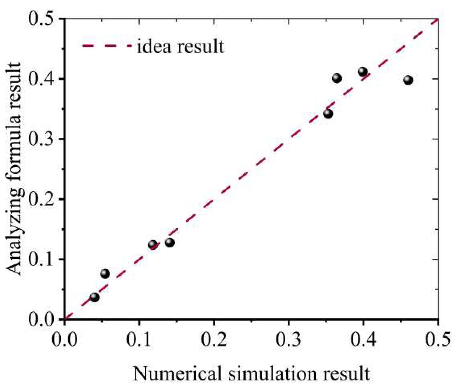
To verify the accuracy of the numerical simulation results, eight representative parameter combinations were randomly selected from Table 3 and compared with the analytical solution proposed by Sun et al. [37]. The comparison results are illustrated in Figure 14. As shown, the predicted settlement depths from the current FEM model closely match the analytical values under the same loading conditions.
Specifically, among the selected cases, the analytical results range from 0.047 m to 0.412 m, while the FEM results range from 0.040 m to 0.460 m. The absolute differences between paired values are generally less than 0.06 m. In terms of relative error, 6 out of 8 cases fall within ±15%. While two of the test cases exhibit slightly larger deviations (above 15%), the overall consistency remains acceptable for model validation purposes, especially considering the complexity of seabed–structure interactions and the absence of full-scale experimental data. This level of agreement confirms the fidelity of the proposed numerical model in capturing the key mechanisms governing DSMV–seabed interaction, thereby supporting its suitability for generating training data for the machine learning model.
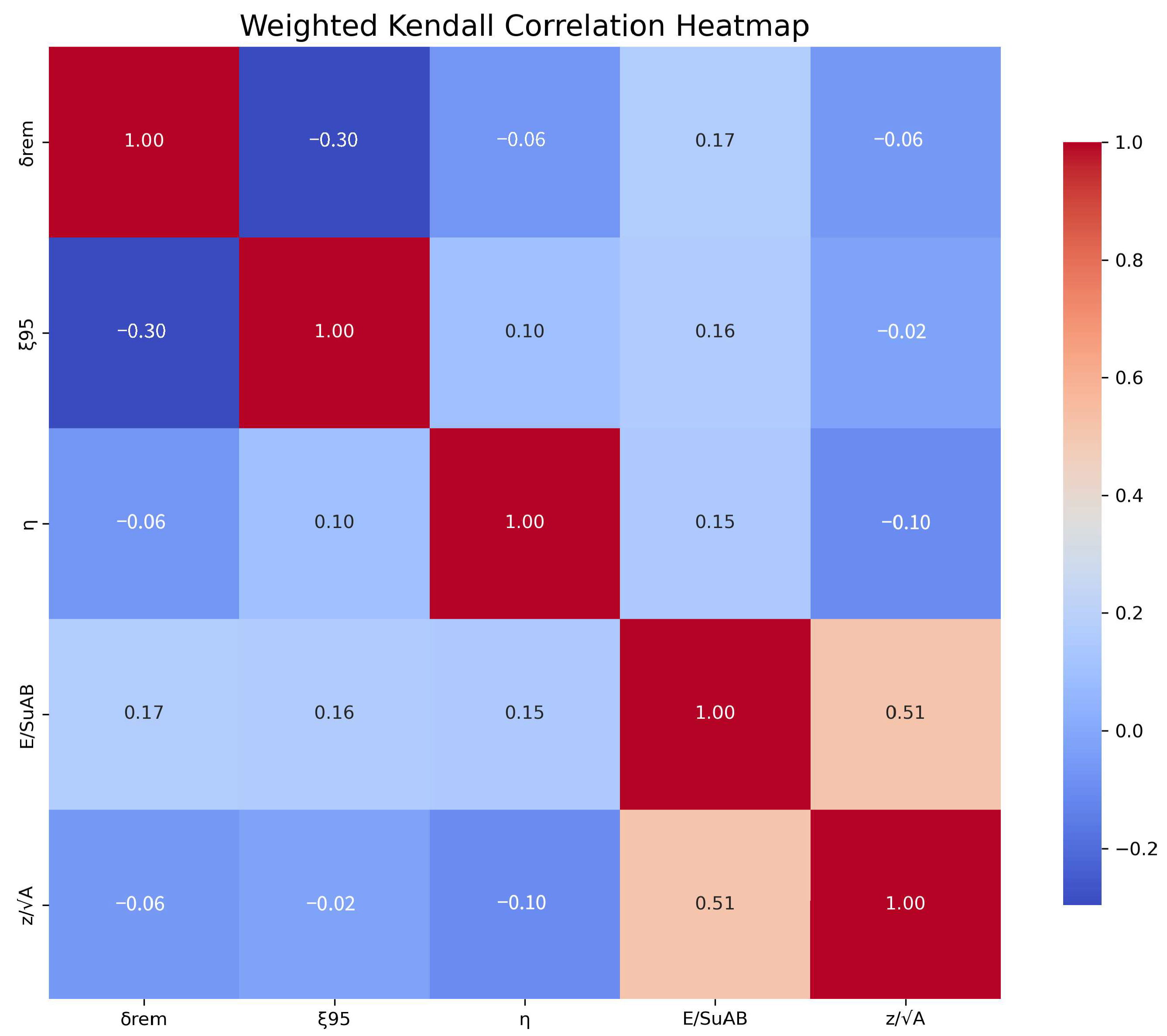
Figure 15 shows a heatmap depicting the Kendall correlation between the input and output parameters. It is clear from the figure that Etotal is positively correlated with z / A . The correlation between Etotal and z / A is very strong, with a correlation coefficient of 0.51. Based on the correlation analysis, the selected set of features is limited and the correlation between the input characteristic parameters and the target output parameters z / A is in accordance with the results of the analysis. Moreover, there is no evidence of multicollinearity between these features. Therefore, we can directly proceed with the training of the random forest model, which corresponds to step (III).
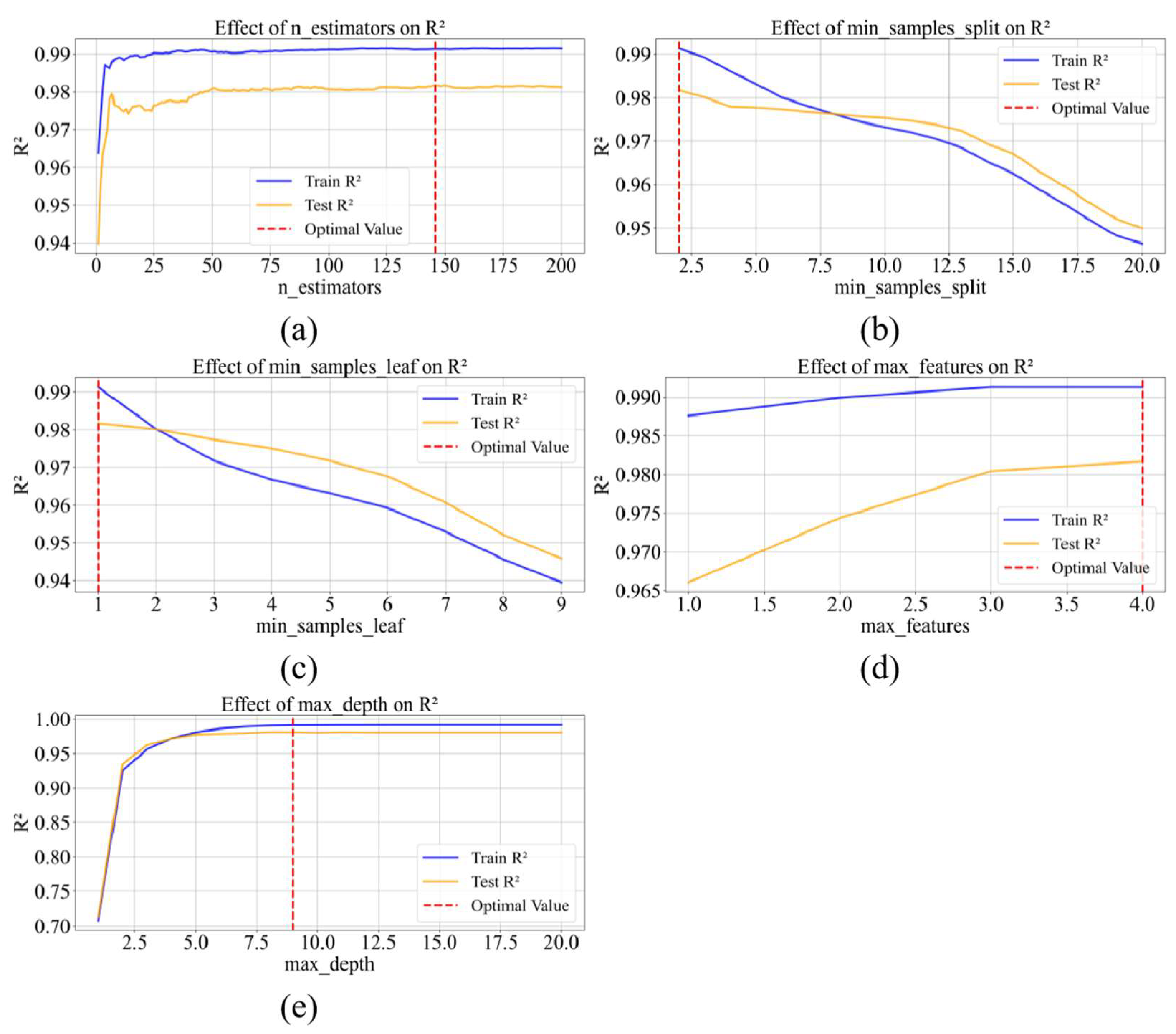
Following the initial model development, a dedicated hyperparameter optimization phase was conducted to enhance the predictive performance of the random forest algorithm. The key hyperparameters subject to tuning included the total number of estimators (n_estimators), the maximum tree depth (max_depth), the upper bound on features considered per split (max_features), and the minimum thresholds for data splits (min_samples_split) and terminal leaf sizes (min_samples_leaf) [77]. Figure 16a–e presents the learning curves reflecting changes in model accuracy (R2) as a function of these critical parameters. An increasing trend in predictive performance is observed with increasing values of (n_estimators), (max_depth), and (max_features), indicating that a more complex ensemble structure generally enhances model capability. In contrast, excessive constraints on internal node splitting or leaf node size tend to restrict model flexibility, thereby reducing predictive accuracy. Based on the comprehensive grid search and curve analysis, the final set of optimal hyperparameters—achieving a balance between accuracy and generalization—is summarized in Table 4.
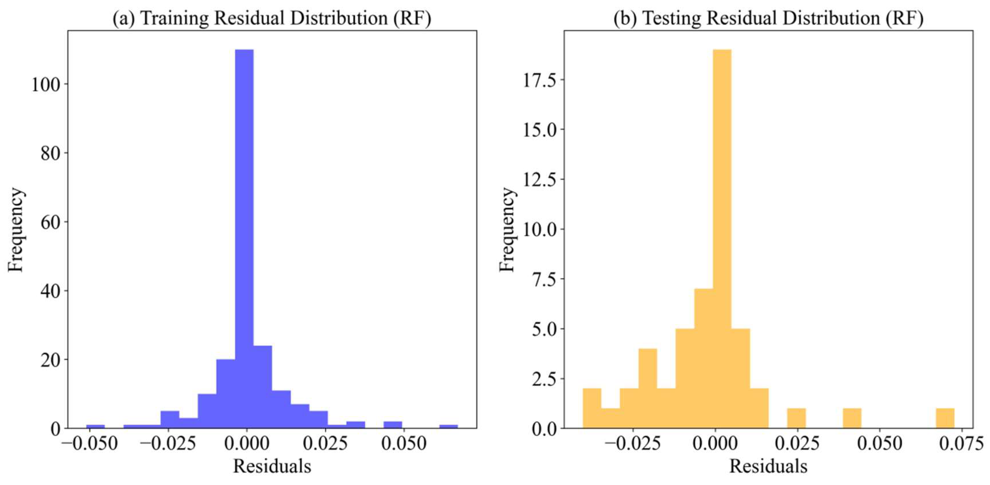
Using the random forest model configured with optimal hyperparameters, predictive performance was assessed on the holdout dataset comprising the remaining 10% of the total samples. The evaluation results are visualized in Figure 17 and Figure 18, which respectively illustrate the alignment between the predicted versus observed values, and the residual distributions for both the training and test sets. The strong convergence between the predicted outputs and true values across datasets indicates excellent model fidelity. The dimensionless penetration resistance coefficients predicted by the model exhibit high agreement with the simulation results, suggesting robust generalizability. Statistical performance metrics, presented in Table 5, further confirm this: the mean absolute error (MAE) remains consistently low across both subsets. Although a few outliers are observed, their impact is marginal, and overall predictive reliability is maintained. Therefore, the model is deemed effective for accurately estimating the maximum penetration depth experienced by the DSMV under varying geotechnical conditions.

4.4. Evaluation of the Prediction Model

This section corresponds to step (IV) in the predictive modeling framework, which focuses on the comprehensive evaluation of model performance. The evaluation is structured into three dimensions: predictive accuracy, generalization capacity, and model robustness. To quantify accuracy, four statistical indicators were employed—the coefficient of determination (R2), mean squared error (MSE), mean absolute error (MAE), and root mean squared error (RMSE)—as summarized in Table 5 [78]. These metrics were computed based on test set predictions to assess the model’s ability to reproduce the dimensionless sinkage depth. The evaluation results confirm that the random forest algorithm achieves consistently high accuracy across all the metrics, indicating its strong capacity to capture the nonlinear relationships governing DSMV penetration resistance. Accordingly, the RF model is a suitable and reliable approach for predicting seabed interaction outcomes under varying geotechnical conditions.
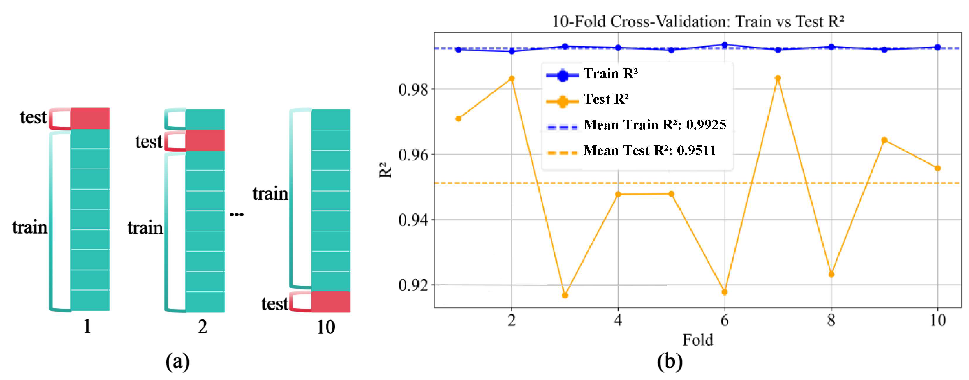
To evaluate the model’s generalizability, a k-fold cross-validation approach was adopted [79]. This technique involves partitioning the dataset into k equally sized subsets; during each iteration, one subset is reserved for validation while the remaining k − 1 subsets are used for training. Repeating this process k times ensures that each sample is used for both training and validation, thereby reducing the variance caused by a single train–test split. For this study, a standard 10-fold cross-validation was applied, which is a widely accepted practice in machine learning applications [80]. The coefficient of determination (R2) was employed as the primary metric to quantify model performance across all folds (Figure 19). The results demonstrate the strong generalizability of the random forest model: on the training set, the R2 values ranged from 0.9919 to 0.9937, yielding an average of 0.9925; on the test set, the R2 values ranged from 0.9168 to 0.9835, with a corresponding average of 0.9511. These consistently high R2 scores confirm that the model maintains robust predictive accuracy, even when exposed to previously unseen data.
To further investigate the stability of the random forest prediction model under stochastic data conditions, a series of 200 independent Monte Carlo simulations was carried out [52,81]. In each iteration, the dataset was randomly partitioned into training and test subsets using a 90:10 split ratio, followed by the computation of normalized regression metrics—the coefficient of determination (R2), root mean squared error (RMSE), and mean absolute error (MAE)—for both subsets. The simulation protocol follows the approach detailed in the literature [52]. The results from the training set show a high degree of consistency across iterations, indicating that the model’s performance is largely unaffected by variations in data partitioning. While minor fluctuations are noted in the test set results, the normalized values of R2, RMSE, and MAE exhibit strong convergence toward 1 as the number of runs approaches 200, as depicted in Figure 20. Across all the simulations, the predictive metrics derived from the training data consistently outperform those derived from the test data, although the discrepancy remains small. This performance pattern underscores the robustness and generalization strength of the proposed model, validating its applicability in diverse geotechnical scenarios.

5. Conclusions

To investigate the sinking patterns and assessment methods of an unloaded DSMV in deep ocean surface soft sediments under complex conditions, this study proposes a dual-method framework that integrates high-fidelity finite element simulations with data-driven machine learning predictions. The FEM model, based on the CEL approach and an improved constitutive law, enables accurate simulation of DSMV–seabed interactions under various sediment and loading conditions. The random forest algorithm is then trained using the FEM dataset to establish a fast and generalizable prediction model for dimensionless settlement depth. This methodological integration significantly improves the accuracy and efficiency of seabed landing safety assessments.
The main findings are summarized as follows:
(1) A high-fidelity CEL finite element model was developed to simulate the landing and penetration behavior of a full-scale DSMV track system under various sediment conditions. The track structure was modeled as a rigid assembly with detailed geometry and contact definitions, while the seabed was represented using a rate-dependent and strain-softening constitutive soil model. This configuration enables realistic capture of nonlinear soil–track interactions and large-deformation responses. The model predictions align well with those of existing studies, confirming its physical realism and engineering applicability.
(2) Parametric analyses revealed that the dimensionless settlement depth decreases with increasing undrained shear strength but increases significantly with higher sensitivity, faster softening rates (i.e., lower ξ95), greater bottoming velocities, and stiffer contact conditions. Contour plots of the plastic strain and shear strain rate revealed that highly sensitive and rapidly loaded sediments, which are the primary contributors to deeper penetration, are more prone to shear localization and intense flow behavior.
(3) The incorporation of a strain-softening and rate-dependent constitutive model allowed for more accurate simulations of strength evolution in deep-sea sediments under dynamic loading. The results show that strain rate effects introduce apparent viscous hardening under fast landing scenarios, partially offsetting strength degradation. However, under high-sensitivity or low-rate conditions, softening dominates, leading to more extensive failure zones and greater settlement.
(4) An RF regression model based on ensemble learning was constructed to predict the dimensionless settlement depth using high-dimensional input features. With the test R2 exceeding 0.94, the random forest model demonstrated strong alignment with simulation results. The feature importance analysis further highlighted strength, strain sensitivity, and descent dynamics as critical predictors validating the model’s ability to identify key physical drivers in the DSMV landing process. Compared with conventional empirical approaches, the RF model demonstrates superior nonlinearity handling and generalization capability.
(5) The proposed integrated framework supports an efficient parameter screening strategy for evaluating settlement sensitivity across various landing scenarios. This approach provides a practical tool for optimizing the DSMV track structure design and descent planning. Future work may extend this framework by incorporating uncertainty quantification and real-time feedback control to support the development of a digital twin for deep-sea landing operations.

6. Limitations

Despite the encouraging results, this study has some limitations. First, due to the high cost and complexity of full-scale deep-sea field testing, the FEM results have not been validated by actual in situ DSMV landing data. Instead, consistency with prior empirical models and scaled laboratory tests has been used as a proxy for validation. Second, the sediment properties used in this study mainly represent ultra-soft clays found in polymetallic nodule regions, which may limit the generalizability of the findings to other seabed types. Future work will incorporate uncertainty quantification, real-time sensor feedback, and in situ data to further enhance the robustness of the proposed framework.

Author Contributions

Conceptualization, Y.Z., Z.X., L.L., Y.S. and X.G.; Data curation, Y.Z. and Q.X.; Formal analysis, Y.Z., Z.X. and J.Y.; Funding acquisition, Z.X., Q.X. and X.G.; Methodology, Z.X. and L.L.; Resources, L.L., J.Y. and X.G.; Software, J.Y.; Supervision, L.L.; Validation, Y.Z.; Writing—original draft, Y.Z. and Z.X.; Writing—review and editing, Y.Z., Z.X., L.L., Q.X., Y.S., J.Y. and X.G. All authors have read and agreed to the published version of the manuscript.

Funding

This research was funded by the National Natural Science Foundation of China, grant numbers 41876066 and 41606084; the Opening Fund of State Key Laboratory of Geohazard Prevention and Geoenvironment Protection (Chengdu University of Technology), grant number SKLGP2019K023; and the National Key Research and Development Program of China, grant number 2024YFC2815400.

Data Availability Statement

Some data, models, or code generated or used during the study are available in a repository online in accordance with the funder’s data retention policies. Other data, models, or code that support the findings of this study are available from the corresponding author upon reasonable request, including the results of the virtual element tests.

Conflicts of Interest

Author Jianghui Yang was employed by the company China Offshore Oil Engineering Corp CNOOC Ltd. The remaining authors declare that the research was conducted in the absence of any commercial or financial relationships that could be construed as a potential conflict of interest.

References

  1. Du, K.; Xi, W.; Huang, S.; Zhou, J. Deep-sea mineral resource mining: A historical review, developmental progress, and insights. Miner. Metall. Explor. 2024, 41, 173–192. [Google Scholar] [CrossRef]
  2. Sha, F.; Xi, M.; Chen, X.; Liu, X.; Niu, H.; Zuo, Y. A recent review on multi-physics coupling between deep-sea mining equipment and marine sediment. Ocean Eng. 2023, 276, 114229. [Google Scholar] [CrossRef]
  3. Sharma, R. Deep-sea mining and the water column: An introduction. In Deep-Sea Mining and the Water Column: Advances, Monitoring and Related Issues; Springer: Cham, Switzerland, 2024; pp. 3–40. [Google Scholar]
  4. Zhang, N.; Zhai, W.K.; Yin, S.Y.; Chen, X.G.; Xia, J.X.; Luan, L.B.; Zhai, A.S. Deep-sea soft soil and deep-sea mining vehicle interaction: From soil properties to locomotion performance. Appl. Ocean Res. 2025, 154, 104372. [Google Scholar] [CrossRef]
  5. Atmanand, M.; Janardhanan, K.; Amuda, K.; Gnanaraj, A.; Rajesh, S.; Muthuvel, P.; Kuttikrishnan, G.; Ramadass, G. Contemporary technological progress in deepsea mining. In Deep-Sea Mining and the Water Column: Advances, Monitoring and Related Issues; Springer: Cham, Switzerland, 2024; pp. 67–89. [Google Scholar]
  6. Leng, D.; Shao, S.; Xie, Y.; Wang, H.; Liu, G. A brief review of recent progress on deep sea mining vehicle. Ocean Eng. 2021, 228, 108565. [Google Scholar] [CrossRef]
  7. Wu, Q.; Yang, J.; Lu, H.; Lu, W.; Liu, L. Effects of heave motion on the dynamic performance of vertical transport system for deep sea mining. Appl. Ocean Res. 2020, 101, 102188. [Google Scholar] [CrossRef]
  8. Shen, Y.J.; Chen, M.F.; Du, Y.L.; Li, M. Key mechanical issues and technical challenges of deep-sea mining development system. Mech. Eng. 2022, 44, 1005–1020. [Google Scholar]
  9. Liu, S.J.; Chang, L.; Yu, D. Status and progress on researches and developments of deep ocean mining equipments. Chin. J. Mech. Eng. 2014, 50, 8–18. [Google Scholar] [CrossRef]
  10. Zhao, H.L.; Sun, Y.F.; Jia, C.; Wei, R.C.; Deng, H.; Wu, T. The sinkage by mining car traveling on deep-sea soft bottom based on Burger’s creep model. Mar. Geol. Quat. Geol. 2024, 44, 179–190. [Google Scholar] [CrossRef]
  11. Hong, S.; Kim, H.W.; Yeu, T.; Choi, J.S.; Lee, T.H.; Lee, J.K. Technologies for safe and sustainable mining of deep-seabed minerals. In Environmental Issues in Deep-Sea Mining: Impacts, Consequences and Policy Perspectives; Springer: Cham, Switzerland, 2019; pp. 95–143. [Google Scholar]
  12. Kang, Y.J.; Liu, S.J. The development history and latest progress of deep-sea polymetallic nodule mining technology. Minerals 2021, 11, 1132. [Google Scholar] [CrossRef]
  13. Rauf, O.; Yang, N.; Chen, M.; Ma, H.X. Evaluation of ground pressure, bearing capacity, and sinkage in rigid-flexible tracked vehicles on characterized terrain in laboratory conditions. Sensors 2024, 24, 1779. [Google Scholar] [CrossRef]
  14. Laughery, S.; Gerhart, G.; Goetz, R. Bekker’s Terramechanics Model for Off-Road Vehicle Research; US Army TARDEC: Hammond, WI, USA, 1990. [Google Scholar]
  15. Bekker, M.G. Introduction to Terrain-Vehicle Systems; University of Michigan Press: Ann Arbor, MI, USA, 1969. [Google Scholar]
  16. Bekker, M.G.; Kitano, M.; Kumagai, K. Theory of Land Locomotion; University of Michigan Press: Ann Arbor, MI, USA, 1969. [Google Scholar]
  17. Agarwal, S.; Senatore, C.; Zhang, T.G.; Kingsbury, M.; Iagnemma, K.; Goldman, D.I.; Kamrin, K. Modeling of the interaction of rigid wheels with dry granular media. J. Terramechanics 2019, 85, 1–14. [Google Scholar] [CrossRef]
  18. Wang, L.; Chen, X.G.; Li, Z.G.; Liu, X.L.; Liu, X.X.; Wang, L.Z.; Yang, W.D. Analysis of traction performance of deep-sea tracked mining vehicles under different grouser pitch-to-height ratios and traveling speeds. Ocean Eng. 2024, 297, 117112. [Google Scholar] [CrossRef]
  19. Kim, Y.H.; Hossain, M.S. Dynamic installation of OMNI-Max anchors in clay: Numerical analysis. Géotechnique 2015, 65, 1037–1096. [Google Scholar] [CrossRef]
  20. Kim, Y.H.; Hossain, M.S.; Wang, D. Effect of strain rate and strain softening on embedment depth of a torpedo anchor in clay. Ocean Eng. 2015, 108, 704–715. [Google Scholar] [CrossRef]
  21. Kim, Y.H.; Hossain, M.S.; Wang, D.; Randolph, M.F. Numerical investigation of dynamic installation of torpedo anchors in clay. Ocean Eng. 2015, 108, 820–832. [Google Scholar] [CrossRef]
  22. Zhao, J.; Jang, B.; Duan, M. On spudcan deep penetration using Eulerian finite element in multi-layer sediments: Soil plug mechanism. Ships Offshore Struct. 2017, 12, 715–721. [Google Scholar] [CrossRef]
  23. Dai, X.; Xu, T.; Chen, J. Physical and mechanical properties of deep oceanic sediments cored from the bottom of Challenger Deep, Mariana Trench. Geofluids 2021, 2021, 9109132. [Google Scholar] [CrossRef]
  24. Li, L.; Li, S.L. Simulation and mechanical characteristics of terramechanics of the surface soil on deep-sea bed. Eng. Mech. 2010, 13, 213–220. [Google Scholar]
  25. Su, Q.; Lv, H.; Yang, J.M.; Sun, P.F. Analysis of the walking performance of tracked deep-sea mining vehicle on soft sediment. Ocean Eng. 2022, 2, 162–168. [Google Scholar]
  26. Einav, I.; Randolph, M.F. Combining upper bound and strain path methods for evaluating penetration resistance. Int. J. Numer. Meth. Eng. 2005, 63, 1991–2016. [Google Scholar] [CrossRef]
  27. Benson, D.J. Computational methods in Lagrangian and Eulerian hydrocodes. Comput. Methods Appl. Mech. Eng. 1992, 99, 235–394. [Google Scholar] [CrossRef]
  28. Wang, J.Y.; Cao, W.G.; Zhai, Y.C. Experimental study of interaction between deep-sea sediments and tracks. Rock Soil Mech. 2011, S2, 274–278. [Google Scholar]
  29. Zhang, W.; Cassidy, M.J.; Tian, Y. Practical large-deformation finite-element method for 3D geotechnical problems involving free surface deformations. Int. J. Geomech. 2020, 20, 04020064. [Google Scholar] [CrossRef]
  30. Liu, M.; Huang, W.X.; Yuan, W.H.; Zhang, W. Modelling the large deformation failure behaviour of unsaturated porous media with a two-phase fully-coupled smoothed particle finite element method. SSRN Electron. J. 2023, 427, 117013. [Google Scholar] [CrossRef]
  31. Yuan, W.; Zhu, J.; Wang, N.; Zhang, W.; Dai, B.; Jiang, Y.; Wang, Y. A dynamic large-deformation particle finite element method for geotechnical applications based on Abaqus. J. Rock Mech. Geotech. Eng. 2023, 15, 1859–1871. [Google Scholar] [CrossRef]
  32. Huang, C.; Qian, J. FEM-BEM modeling of dynamic responses of a fluid-filled lined tunnel under a water hammer. J. Eng. Mech. 2024, 150, 04022045. [Google Scholar] [CrossRef]
  33. Janarthanan, C.; Kuttikrishnan, G.; Sundaramoorthi, V.; Chandran, V.; Ramadass, G.A. Deep Sea Soil Sinkage Simulation and Experimental Studies for Development of Deep Water Mining Machine. Mar. Technol. Soc. J. 2022, 56, 72–82. [Google Scholar] [CrossRef]
  34. Amudha, K.; Reshma, K.V.; Ramesh, N.R.; Deepak, C.R.; Ramadass, G.A.; Atmanand, M.A. Estimation of sinkage and breakout forces for tracked vehicle for soft soils. In Proceedings of the OCEANS 2014—TAIPEI, Taipei, Taiwan, 7–10 April 2014; pp. 1–7. [Google Scholar] [CrossRef]
  35. Janarthanan, C.; Muruganandhan, R.; Gopkumar, K. Design and multi-body dynamic analysis of inline and offset track configuration in deep-sea mining vehicles for enhanced traction in soft seabed. J. Terramechanics 2024, 116, 100999. [Google Scholar] [CrossRef]
  36. Sun, P.; Lu, H.; Yang, J.; Deng, L.; Liu, M.; Li, S. Numerical study on multiple parameters of sinkage simulation between the track plate of the deep-sea mining vehicle and the seafloor soil. J. Mar. Sci. Eng. 2022, 10, 1680. [Google Scholar] [CrossRef]
  37. Sun, P.; Lu, H.; Yang, J.; Xu, Z. A numerical investigation on the sinkage of the deep-sea mining vehicle based on a modified constitutive soil model. ASME J. Offshore Mech. Arct. Eng. 2025, 147, 022101. [Google Scholar] [CrossRef]
  38. Luan, L.; Chen, X.; Kouretzis, G.; Ding, X. Dynamic seabed stresses due to moving deep-sea mining vehicles. Comput. Geotech. 2023, 157, 105356. [Google Scholar] [CrossRef]
  39. Xia, M.; Lu, H.; Yang, J.; Sun, P. Multi-Body Dynamics Modeling and Straight-Line Travel Simulation of a Four-Tracked Deep-Sea Mining Vehicle on Flat Ground. J. Mar. Sci. Eng. 2023, 11, 1005. [Google Scholar] [CrossRef]
  40. Liu, Y.Y.; Wan, Z.; Quan, D.G.; Liu, Y.F.; Jia, Y.G.; Zhu, N. Analysis of bearing capacity of consolidated clay under the track load of deep-sea mining vehicle. Mar. Georesour. Geotechnol. 2024, 43, 508–523. [Google Scholar] [CrossRef]
  41. Tho, K.K.; Leung, C.F.; Chow, Y.K.; Swaddiwudhipong, S. Eulerian finite-element simulation of spudcan–pile interaction. Can. Geotech. J. 2013, 50, 595–608. [Google Scholar] [CrossRef]
  42. Gonzalez, R.; Iagnemma, K. DeepTerramechanics: Terrain classification and slip estimation for ground robots via deep learning. arXiv 2018, arXiv:1806.07379. [Google Scholar] [CrossRef]
  43. Chavez-Garcia, R.O.; Guzzi, J.; Gambardella, L.M.; Giusti, A. Learning ground traversability from simulations. IEEE Robot. Autom. Lett. 2018, 3, 1695–1702. [Google Scholar] [CrossRef]
  44. Zhang, N.; Zhai, W.; Yin, S.; Song, Y.; Chen, X.; Guo, C.; Ma, Y. Study of the tractive performance of a deep-sea mining vehicle based on the soil failure mode. Int. J. Geomech. 2025, 25, 04025013. [Google Scholar] [CrossRef]
  45. Zande, M.; Smith, J.; Thompson, R. Coupled numerical–experimental framework for track–soil interaction in planetary rovers. J. Terramechanics 2024, 101, 35–43. [Google Scholar] [CrossRef]
  46. White, D.; Randolph, M. Seabed characterisation and models for pipeline-soil interaction. Int. J. Offshore Polar Eng. 2007, 17, 193–204. [Google Scholar]
  47. Xiao, Z.; Fu, D.F.; Zhou, Z.F.; Lu, Y.; Yan, Y. Effects of strain softening on the penetration resistance of offshore bucket foundation in nonhomogeneous clay. Ocean Eng. 2019, 193, 106594. [Google Scholar] [CrossRef]
  48. Xie, Q.; Xu, Q.; Xiu, Z.; Liu, L.; Du, X.; Yang, J.; Liu, H. Convenient method for large-deformation finite-element simulation of submarine landslides considering shear softening and rate correlation effects. J. Mar. Sci. Eng. 2024, 12, 81. [Google Scholar] [CrossRef]
  49. Guo, X.; Liu, Z.; Zheng, J.; Luo, Q.; Liu, X. Bearing capacity factors of T-bar from surficial to stable penetration into deep-sea sediments. Soil Dyn. Earthq. Eng. 2023, 165, 107671. [Google Scholar] [CrossRef]
  50. Pham, B.T.; Hoang, T.A.; Nguyen, D.M.; Bui, D.T. Prediction of shear strength of soft soil using machine learning methods. Catena 2018, 166, 181–191. [Google Scholar] [CrossRef]
  51. Phoon, K.K.; Zhang, W.G. Future of machine learning in geotechnics. Georisk 2023, 17, 7–22. [Google Scholar] [CrossRef]
  52. Nguyen, M.; Pham, B.; Tuyen, T.; Yen, H.; Prakash, I.; Vu, T.; Chapi, K.; Shirzadi, A. Development of an artificial intelligence approach for prediction of consolidation coefficient of soft soil: A sensitivity analysis. Open Constr. Build. Technol. J. 2019, 13, 178–188. [Google Scholar] [CrossRef]
  53. Shahani, N.M.; Kamran, M.; Zheng, X.G.; Liu, C.C.; Guo, X.W. Application of gradient boosting machine learning algorithms to predict uniaxial compressive strength of soft sedimentary rocks at Thar Coalfield. Adv. Civ. Eng. 2021, 2021, 2565488. [Google Scholar] [CrossRef]
  54. Shao, W.; Yue, W.H.; Zhang, Y.; Zhou, T.X.; Zhang, Y.T.; Dang, Y.B.; Wang, H.Y.; Feng, X.H. The application of machine learning techniques in geotechnical engineering: A review and comparison. Mathematics 2023, 11, 3976. [Google Scholar] [CrossRef]
  55. Guo, X.S.; Meng, X.S.; Han, F.H.; Zhang, H.; Liu, X.L. Assessing the strength of deep-sea surface ultrasoft sediments with T-bar penetration: A machine learning approach. Eng. Geol. 2024, 338, 107632. [Google Scholar] [CrossRef]
  56. Sagi, O.; Rokach, L. Ensemble learning: A survey. Wiley Interdiscip. Rev. Data Min. Knowl. Discov. 2018, 8, e1249. [Google Scholar] [CrossRef]
  57. Yin, J.N.; Li, N. Ensemble learning models with a Bayesian optimization algorithm for mineral prospectivity mapping. Ore Geol. Rev. 2022, 145, 104916. [Google Scholar] [CrossRef]
  58. Zhang, D.M.; Zhang, J.Z.; Huang, H.W.; Qi, C.C.; Chang, C.Y. Machine learning-based prediction of soil compression modulus with application of 1D settlement. J. Zhejiang Univ. Sci. A 2020, 21, 430–444. [Google Scholar] [CrossRef]
  59. Breiman, L. Random forests. Mach. Learn. 2021, 45, 5–32. [Google Scholar] [CrossRef]
  60. Graw, J.H.; Wood, W.T.; Phrampus, B.J. Predicting global marine sediment density using the random forest regressor machine learning algorithm. J. Geophys. Res. Solid Earth 2021, 126, e2020JB020135. [Google Scholar] [CrossRef]
  61. Benson, D.J.; Okazawa, S. Contact in a multi-material Eulerian finite element formulation. Comput. Methods Appl. Mech. Eng. 2004, 193, 4277–4298. [Google Scholar] [CrossRef]
  62. Li, T.; Tang, X.W.; Wang, Z. Experimental Study on Unconfined Compressive and Cyclic Behaviors of Mucky Silty Clay with Different Clay Contents. Int. J. Civ. Eng. 2019, 17, 841–857. [Google Scholar] [CrossRef]
  63. Aubeny, C.P.; Shi, H. Effect of rate-dependent soil strength on cylinders penetrating into soft clay. IEEE J. Ocean. Eng. 2007, 32, 49–56. [Google Scholar] [CrossRef]
  64. Zhou, H.; Randolph, M.F. Computational techniques and shear band development for cylindrical and spherical penetrometers in strain-softening clay. Int. J. Geomech. 2007, 7, 287–295. [Google Scholar] [CrossRef]
  65. Zhou, H.; Randolph, M.F. Numerical investigations into cycling of full-flow penetrometers in soft clay. Géotechnique 2009, 59, 801–812. [Google Scholar] [CrossRef]
  66. Zhu, H.; Randolph, M.F. Numerical analysis of a cylinder moving through rate-dependent undrained soil. Ocean Eng. 2010, 38, 943–953. [Google Scholar] [CrossRef]
  67. Boukpeti, N.; White, D.J.; Randolph, M.F.; Low, H.E. Strength of fine grained soils at the solid-fluid transition. Géotechnique 2012, 62, 213–226. [Google Scholar] [CrossRef]
  68. Biscontin, G.; Pestana, J.M. Influence of peripheral velocity on vane shear strength of an artificial clay. Geotech. Test. J. 2001, 24, 423–429. [Google Scholar] [CrossRef]
  69. Randolph, M.F. Characterisation of soft sediments for offshore applications. In Proceedings of the 2nd International Conference on Site Characterization, Rotterdam, The Netherlands, 19–22 September 2004; pp. 209–232. [Google Scholar]
  70. Dutta, S.; Hawlader, B.; Phillips, R. Finite element modeling of partially embedded pipelines in clay seabed using coupled Eulerian-Lagrangian method. Can. Geotech. J. 2015, 52, 58–72. [Google Scholar] [CrossRef]
  71. Dutta, S.; Hawlader, B. Pipeline soil-water interaction modelling for submarine landslide impact on suspended offshore pipelines. Géotechnique 2019, 69, 29–41. [Google Scholar] [CrossRef]
  72. Hansbo, S. A new approach to the determination of the shear strength of clay by the fall-cone test. Proc. Swed. Geotech. Inst. 1957, 14, 1–46. [Google Scholar]
  73. Uddin, M.F.; Lee, J.; Rizvi, S.; Hamada, S. Proposing Enhanced Feature Engineering and a Selection Model for Machine Learning Processes. Appl. Sci. 2018, 8, 646. [Google Scholar] [CrossRef]
  74. O’Loughlin, C.D.; Richardson, M.D.; Gaudin, C.; Randolph, M.F. Penetration of dynamically installed anchors in clay. Géotechnique 2013, 63, 909–919. [Google Scholar] [CrossRef]
  75. Wei, M.D.; Meng, W.Z.; Dai, F.; Wu, W. Application of machine learning in predicting the rate-dependent compressive strength of rocks. J. Rock Mech. Geotech. Eng. 2022, 14, 1356–1365. [Google Scholar] [CrossRef]
  76. Zhang, W.G.; Wu, C.Z.; Zhong, H.Y.; Li, Y.Q.; Wang, L. Prediction of undrained shear strength using extreme gradient boosting and random forest based on Bayesian optimization. Geosci. Front. 2021, 12, 469–477. [Google Scholar] [CrossRef]
  77. Abdi, Y.; Momeni, E.; Armaghani, D.J. Elastic modulus estimation of weak rock samples using random forest technique. Bull. Eng. Geol. Environ. 2023, 82, 185. [Google Scholar] [CrossRef]
  78. Zhou, J.; Qiu, Y.G.; Armaghani, D.J.; Zhang, W.G.; Li, C.Q.; Zhu, S.L.; Tarinejad, R. Predicting TBM penetration rate in hard rock condition: A comparative study among six XGB-based metaheuristic techniques. Geosci. Front. 2021, 12, 101093. [Google Scholar] [CrossRef]
  79. Yan, T.; Shen, S.L.; Zhou, A.N.; Chen, X.S. Prediction of geological characteristics from shield operational parameters by integrating grid search and K-fold cross validation into stacking classification algorithm. J. Rock Mech. Geotech. Eng. 2022, 14, 1292–1303. [Google Scholar] [CrossRef]
  80. Zhang, P.; Yin, Z.Y.; Jin, Y.F.; Chan, T.H. A novel hybrid surrogate intelligent model for creep index prediction based on particle swarm optimization and random forest. Eng. Geol. 2020, 265, 105328. [Google Scholar] [CrossRef]
  81. Ly, H.B.; Nguyen, T.A.; Pham, B.T. Estimation of soil cohesion using machine learning method: A random forest approach. Adv. Civ. Eng. 2021, 2021, 8873993. [Google Scholar] [CrossRef]
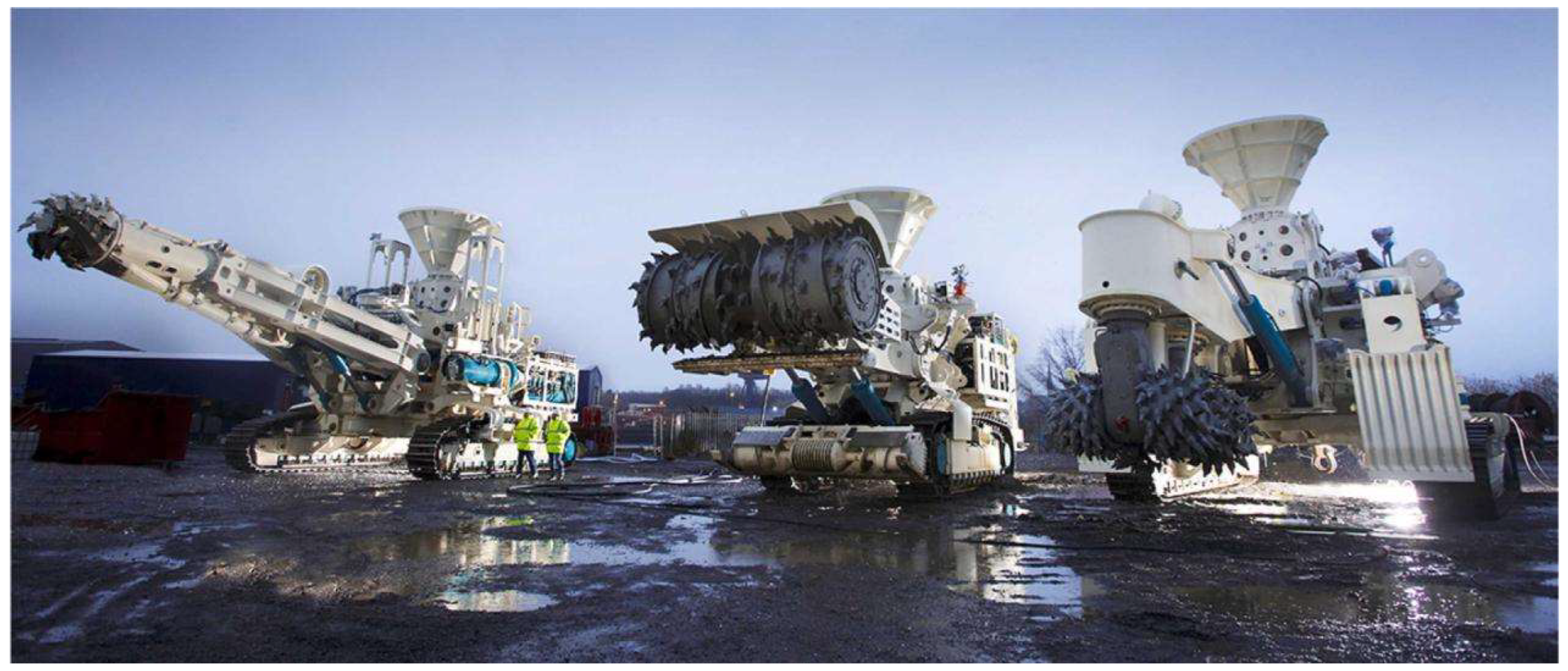
Figure 1. Mining vehicles of polymetallic sulfides developed by Nautilus Minerals Commence (Source: https://dsmobserver.com/2017/07/nautilus-png-submerged-trials/ accessed on 5 December 2024).
Jmse 13 01584 g001
Figure 2. Continuum deformation using the (a) Lagrangian and (b) Eulerian methods.
Jmse 13 01584 g002
Figure 3. Distribution and variation in the shear strength (Pa) of Sample Ⅲ at different moments of the numerical modeling process: (a) Initial moment; (b) Penetration process; (c) Final moment.
Jmse 13 01584 g003
Figure 4. Comparison between the numerical simulation results and the fall cone test results.
Jmse 13 01584 g004
Figure 5. Geometric parameters of the track and track plate: (a) Full-size track geometry model; (b) Track plate geometry model; (c) Overall diagram of the model.
Jmse 13 01584 g005
Figure 6. Mesh sensitivity analysis results.
Jmse 13 01584 g006
Figure 7. Variation in the maximum DSMV sinkage depth with increasing undrained shear strength magnitude and distribution: (a) Different surface shear strengths; (b) Different shear strength enhancement factors.
Jmse 13 01584 g007
Figure 8. Accumulated plastic shear strain under low vs. high ks.
Jmse 13 01584 g008
Figure 9. Relationship between the softening effect parameter and the maximum depth of sinkage of the DSMV under the same load and shear strength conditions: (a) Different soil sensitivities; (b) Different plastic strain parameters; (c) Different soil viscosities.
Jmse 13 01584 g009
Figure 10. Shear strength contours under different viscosity coefficients (η).
Jmse 13 01584 g010
Figure 11. Relationship between the maximum sinkage of the DSMV and its dynamic parameters under the same soil parameter conditions: (a) Different wet weights of mining vehicles; (b) Different bottom contact speeds; (c) Different contact areas.
Jmse 13 01584 g011
Figure 12. Soil velocity field at low and high DSMV bottoming velocities.
Jmse 13 01584 g012
Figure 13. Conceptual diagram of the random forest modeling principle.
Jmse 13 01584 g013
Figure 14. Comparison of the numerical simulation results with the analytical equation results.
Jmse 13 01584 g014
Figure 15. Heatmap of correlation coefficients.
Jmse 13 01584 g015
Figure 16. Variation in random forest accuracy versus key hyperparameters: (a) N_Estimators; (b) Max_Depth; (c) Min_Samples_Split; (d) Min_Samples_Leaf; (e) Max_Features.
Jmse 13 01584 g016
Figure 17. (a) Proximity of the training set actual and predicted values and (b) proximity of the testing set actual and predicted values.
Jmse 13 01584 g017
Figure 18. Error quantification analysis.
Jmse 13 01584 g018
Figure 19. 10-fold cross-validation of the established prediction model: (a) schematic diagram of the 10-fold cross validation principle; (b) 10-fold cross validation results.
Jmse 13 01584 g019
Figure 20. Normalized accuracy and errors from 200 runs of Monte Carlo simulation for the established prediction model: (a) normalized convergence values of R2; (b) normalized convergence values of RMSE; (c) normalized convergence values of MAE.
Jmse 13 01584 g020
Table 1. Physical and mechanical characteristics of the sample soil.
Sample No.Submerged Density
(kg/m3)
Cohesion
(kPa)
Elastic Modulus (MPa)Soil Sensitivity Poission’s Ratio
I590157.5100.49
II5204.22.1420.49
III6608.24.116.40.49
IV180115.58.50.49
Table 2. Mesh sensitivity parameter setting.
Case 1Case 2Case 3Case 4Case 5Case 6
Center region0.020.030.040.050.060.08
Edge region0.50.50.50.50.50.5
Number of elements1,905,1201,503,6631,248,9121,091,475940,212787,626
Stable time increment (s)4.89 × 10−57.34 × 10−59.78 × 10−51.22 × 10−41.47 × 10−41.96 × 10−4
Table 3. Parameter ranges in the sample data.
m (kg)A (m2)vi (m/s)ηStξ95Su0 (Pa)K (Pa/m)
25001.871011020000
30002.1820.0121525001000
45002.530.042.52030002000
65002.8140.0532550002500
85003.1250.13.333060003000
9000 60.154407500
10,500 7 5509000
8 8 10,000
10
Table 4. The corresponding values of the optimal hyperparameters.
ParametersN_EstimatorsMax_DepthMin_Samples_SplitMin_Samples_LeafMax_Features
Value1469214
Table 5. Evaluation metrics and their statistical values for the established prediction models.
Evaluation MetricsR2MSEMAERMSE
Training set0.99140.00010.00660.0120
Testing set0.98070.00030.01040.0173
Disclaimer/Publisher’s Note: The statements, opinions and data contained in all publications are solely those of the individual author(s) and contributor(s) and not of MDPI and/or the editor(s). MDPI and/or the editor(s) disclaim responsibility for any injury to people or property resulting from any ideas, methods, instructions or products referred to in the content.