Optimization of Configuration Design for Underwater Dam Defect Detection Vehicles

Abstract

Hydropower stations and dams play a crucial role in water management, ecology, and energy. To meet the requirements of underwater dam defect detection, this study develops a streamlined underwater vehicle design and operational framework inspired by bionic principles. A parametric modeling approach was employed to propose the vehicle’s streamlined configuration. Using CFD simulations, hydrodynamic coefficients were calculated and validated through towing experiments in a pool. The hydrodynamic stability of the vehicle was assessed and verified through these analyses. Additionally, various configurations were generated using a free deformation method. An optimization function was established with resistance and stability as the objectives, and the optimal result was derived based on the function’s calculation outcomes. The study designed a high-metacentric underwater vehicle, inspired by the seahorse’s shape, and introduced a novel stability evaluation method. Simulations were conducted to analyze the vehicle’s variable attack angle, drift angle, pitching, and rotational motion at a forward three-throttle speed. The results demonstrate that the vehicle achieves static stability in both the horizontal and vertical planes, as well as dynamic stability in the vertical plane, but exhibits limited dynamic stability in the horizontal plane. After optimizing the original configuration, the forward resistance was reduced by 2.15%, while the horizontal plane dynamic stability criterion C_H was improved by 35.29%.

1. Introduction

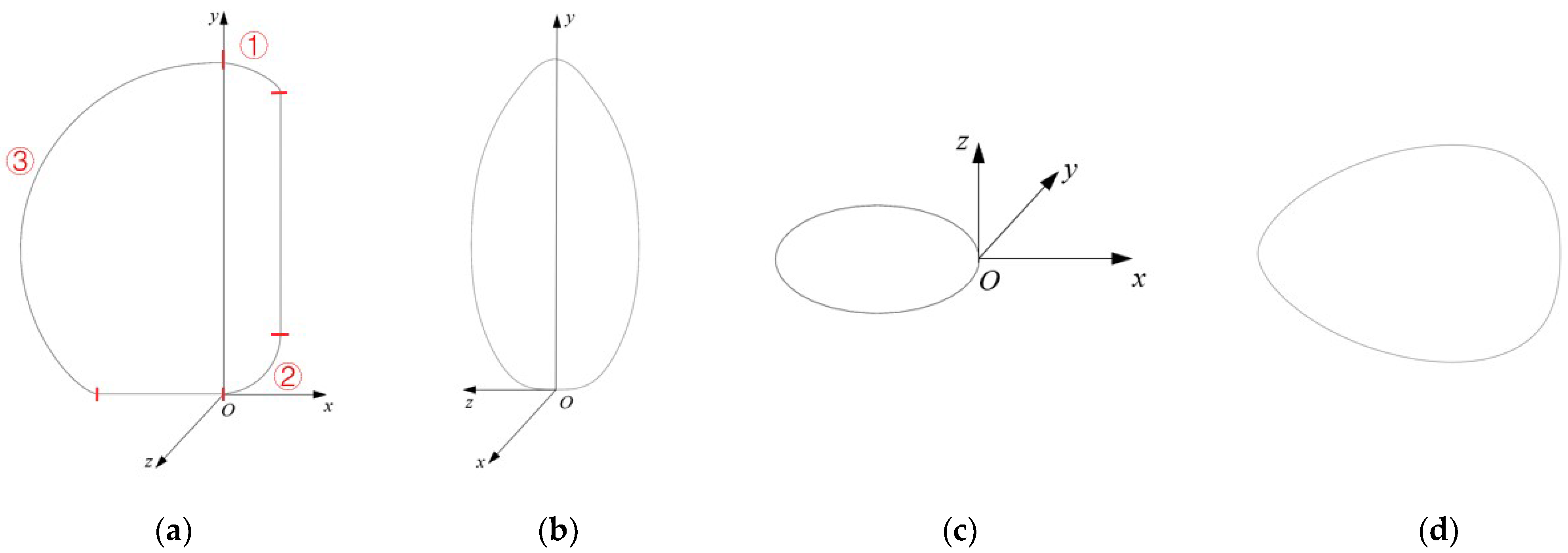
Hydropower stations and reservoir dams are critical national infrastructure, serving functions such as water resource management, ecological restoration, flood control, power generation, and transportation [1,2,3], as shown in Figure 1. However, prolonged underwater immersion, combined with environmental erosion, material aging, loading and temperature variations, chemical corrosion, and hydraulic fracturing, often leads to structural issues such as cracks [4,5,6,7] and cavitation erosion [8]. These types of damage accumulate over time, reducing structural integrity and potentially causing catastrophic failures [9,10]. Remotely operated vehicles (ROVs) are widely used for the underwater inspection of dams, offering comprehensive optical and acoustic scanning to monitor and measure key areas closely. Effective ROV design prioritizes low drag, high maneuverability, and structural strength [11]. Typically, ROVs feature streamlined or open-frame structures, with the latter being the most common for dam inspections [12]. Examples include the French ECA ROV H800 [13], the U.S.-based Seabotix LBV30, Norway’s Argus Mariner, Spain’s University of Girona Ictineu ROV [14], Denmark’s MacArtney FOCUS series, and the UK’s Saab Seaeye Panther Plus. Despite their utility, existing open-frame ROVs often fall short in meeting the demands of rapid deep-water dam inspections due to posture instability and limited detection accuracy. Streamlined ROVs, by contrast, excel in fast underwater detection thanks to their superior attitude control, greater maneuverability, and enhanced resistance to flow disturbances. This paper focuses on designing a streamlined underwater vehicle configuration and evaluating its performance through detailed analysis.

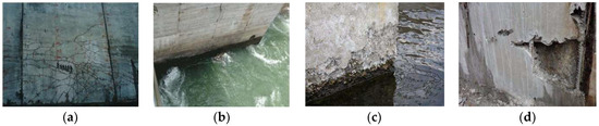
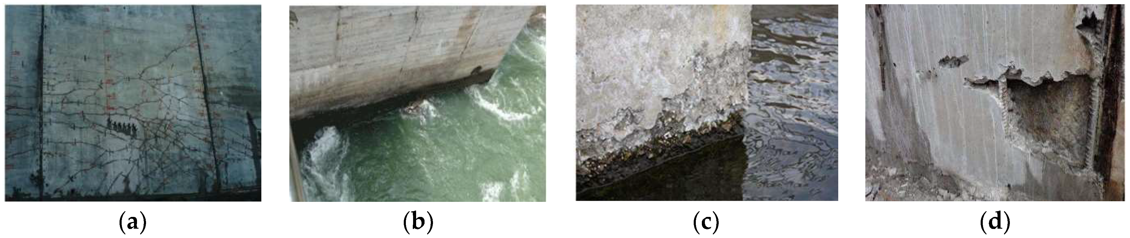
Figure 1. The common defects observed in the dam bodies of hydropower stations include (a) cracks, (b) water leakage, (c) surface erosion, and (d) tendon leakage.

Over millions of years, highly adaptable creatures have evolved with specialized body shapes and locomotion patterns suited to their environments. Inspired by these adaptations, bionics provides valuable insights for designing and improving vehicles to operate effectively in complex working conditions [15,16]. Research in bionics is primarily divided into two areas: materials and structures. In the field of underwater vehicles, materials bionics focuses on mimicking the layered surfaces of aquatic organisms. For example, Li Wen’s team at Beihang University developed a synthetic flexible sharkskin membrane and conducted hydrodynamic experiments to study its performance [17]. Similarly, David Kisailus’s research group at the University of California reviewed the development of multi-scale toughening mechanisms in biological materials and their biomimetic counterparts, highlighting the unique strengthening strategies employed by various organisms [18]. Structural bionics, on the other hand, investigates the morphology, motion, and propulsion mechanisms of animals like crabs [19], fish fins [20,21], jellyfish [22], manta rays [23], snakes [24], and octopuses [25,26]. These studies inspire the design of vehicles capable of adapting to underwater environments by leveraging the structural and functional advantages observed in these species.

This paper focuses on the design of a streamlined ROV for underwater dam inspection, inspired by structural bionics principles. The ROV is required to move vertically along dam surfaces with precision, operate efficiently at low speeds, and perform stationary tasks underwater. As illustrated in Figure 2, three bionic research models were selected to meet these requirements.

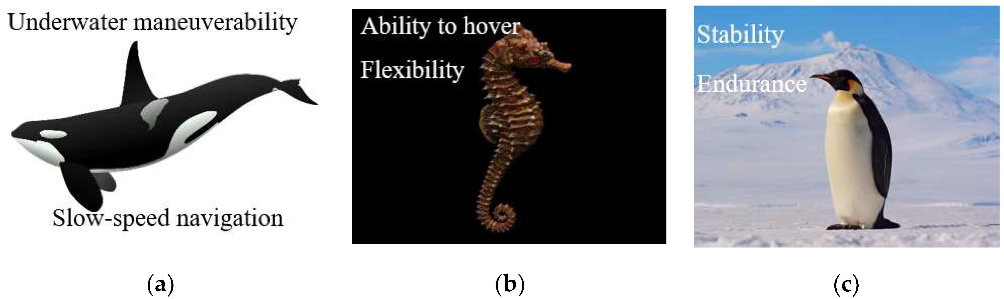
Figure 2. Bionic models for streamlining: (a) killer whale, (b) seahorse, (c) penguin.

Killer whales utilize their vertical tail fins for accelerated swimming, achieving powerful forward and backward propulsion. However, this comes at the cost of reduced flexibility, limiting their ability to perform agile steering and complex movements. Their muscular structure supports high-speed pursuits and long migrations but compromises non-lateral maneuverability. Penguins, on the other hand, have flippers resembling those of seals—broad and flat to enhance propulsion. Compared to fish fins, however, penguin flippers have fewer joints and simpler muscle control, resulting in limited flexibility and reduced capabilities for rapid turns or precise movements.

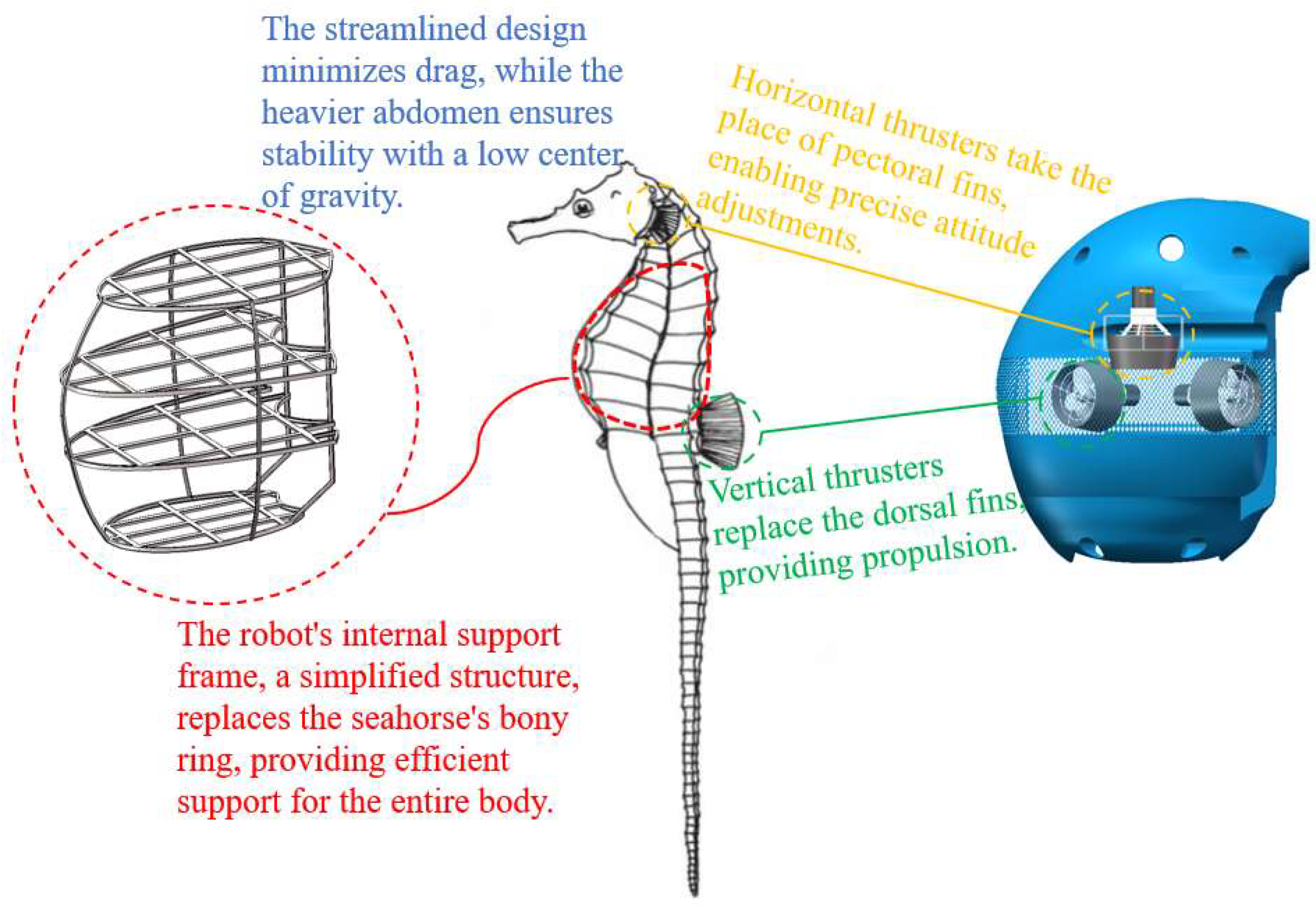
Considering the design requirements of lightweight construction, high stability, and modularity, seahorses were ultimately chosen as the bionic model for configuration. Unlike fast-swimming creatures, seahorses move vertically in the water, a capability supported by their unique anatomy. Their lack of a swim bladder and rigid bony plates limit their swimming speed but enable exceptional hovering ability. Seahorses maintain a stable vertical posture by swinging their dorsal fins and adjusting fin angles for propulsion, while their flexible tails bend to maintain balance. Their heavy abdomen provides a low center of gravity, enhancing stability, while their streamlined body minimizes water resistance and reduces posture disruption.

The preliminary design concept is illustrated in Figure 3 [27]. The high metacentric design ensures that the underwater vehicle maintains a predominantly vertical posture, mimicking the upright movement of a seahorse to enhance maneuverability and facilitate navigation through complex underwater environments. Horizontal and vertical propulsion devices replicate the seahorse’s dorsal fin vibrations and pectoral fin steering, providing thrust and enabling precise attitude adjustments. The rigid bony rings of the seahorse, which protect their internal organs and minimize drag, inspire the vehicle’s structural design. The internal configuration features a simplified support frame that stabilizes the entire body while accommodating equipment, ensuring ease of integration and transport.

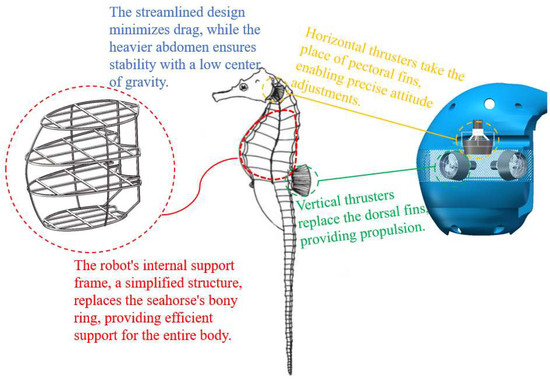
Figure 3. Preliminary design of the underwater vehicle’s streamlined configuration.

The remainder of this paper is organized as follows: Section 2 presents the scientific modeling of the streamlined configuration using specific mathematical equations and outlines the overall design and operational flow of the underwater robot. In Section 3, computational fluid dynamics (CFD) simulations are used to evaluate static stability and dynamic stability. In Section 4, an optimization function is developed to determine the optimal configuration and enhance the dynamic stability in the horizontal plane. Finally, a conclusion is provided based on the above research.

2. Configuration Design of an Underwater Inspection Vehicle for Dams

The above configuration is only a preliminary design, and it is necessary to realize the scientific modeling of the streamline configuration with specific mathematical equations.

2.1. Fundamental Theory

The B-spline method, originally proposed by Schoenberg and derived from the Bessel curve, retains the advantages of the Bessel curve while enabling localized modifications without altering the overall shape. This method allows for efficient curve or surface representation using fewer control points, making it one of the most widely used mathematical approaches today [28,29].

The expression of the B-spline curve of degree k is as follows:

$$L(u)={\displaystyle \sum _{i=0}^n{N}_{i,k}(u)e_i }0\le u\le 1$$

(1)

Non-uniform rational B-splines (NURBSs) are an important extension based on B-spline curves. The NURBS curve is defined as follows:

$$C\left(u\right)={\displaystyle \frac{{\displaystyle \sum _{i=0}^n{N}_{i,k}\left(u\right)e_i{\omega }_i}}{{\displaystyle \sum _{i=0}^n{N}_{i,k}\left(u\right){\omega }_i}}}\left(0\le u\le 1\right)$$

(2)

NURBS surfaces of degree k in u and degree q in v are two-parameter piecewise rational functions of the following form:

$$S\left(u,v\right)={\displaystyle \frac{{\displaystyle \sum _{i=0}^n{\displaystyle \sum _{j=0}^m{N}_{i,k}\left(u\right)N_{j,q}\left(v\right)}}{e}_{i,j}{\omega }_{i,j}}{{\displaystyle \sum _{i=0}^n{\displaystyle \sum _{j=0}^m{N}_{i,k}\left(u\right)N_{j,q}\left(v\right){\omega }_{i,j}}}}}$$

(3)

The NURBS interpolation algorithm constructs a NURBS curve by interpolating a set of arbitrary data, including data point coordinates and guiding vectors. This process ensures that the generated curve or surface strictly adheres to specified data constraints, passing through each data point and aligning with the designated guiding vectors at specific locations.

2.2. Design Procedure

In this paper, the three-dimensional configuration of the non-rotating body is designed, with its contour lines represented mathematically in three principal directions: the transverse section, horizontal plane, and longitudinal section. Due to the lack of complete symmetry among these directions, the asymmetric surfaces are divided into multiple segments to construct the streamlined surface of the vehicle. The coordinate system for this streamlined configuration is illustrated in Figure 4. The standard rectangular coordinate system O-xyz is employed, where the origin O is located at the right end of the bottom surface, and the x, y, and z axes correspond to the forward, vertical, and lateral directions of the configuration, respectively.

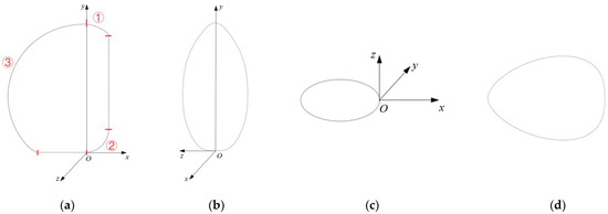
Figure 4. Standard rectangular coordinate system for streamline configuration: (a) frontal view, (b) side view, (c) elevation view, and (d) semi-elevation horizontal profile curve.

The asymmetric section curve cannot be represented by a single mathematical equation, so it is designed in segments. As shown in Figure 4a, the transverse section curve is composed of three curves (ellipse, circle, and NURBS) and two straight lines, with each segment defined parametrically. Only one-half of this symmetric curve is expressed, and the starting and ending tangents are perpendicular to the axis of symmetry. Except for the cross-section, other curves are symmetric. Irregular segments are represented by NURBS curves, which are generated through interpolation using specified data points and defined endpoints. According to the design requirements, these equations for various profile curves are used to construct the profile lines. Using NURBS surface functions and lofting techniques, a 3D model of the vehicle is created, as shown in Figure 4.

2.3. Overall Design

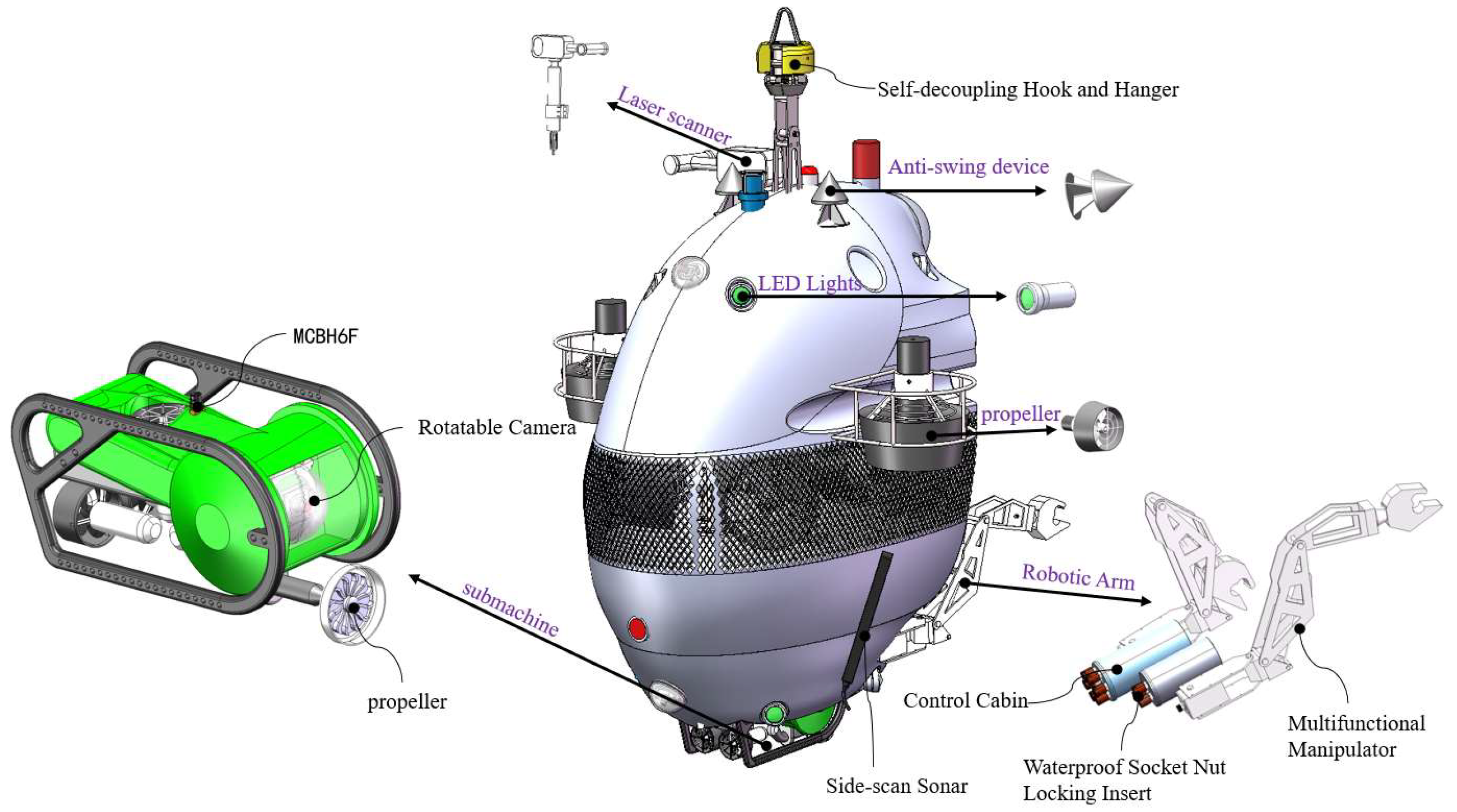
Based on the design plan, the underwater vehicle measures 1.3 m in length, 0.9 m in width, and 1.5 m in height, with an approximate volume of 1 m³ and a total weight of around 180 kg. The design incorporates micro-positive buoyancy, as illustrated in Figure 5.

Figure 5. Vehicle overall scheme layout.

The vehicle is equipped with a self-disconnecting hanger device on its top, facilitating lifting and protecting the umbilical cable. To ensure underwater stability, the relative positioning of the center of buoyancy and the center of gravity must be carefully designed. Ideally, these centers should align vertically, with the center of buoyancy above the center of gravity, enhancing both static and dynamic stability. Because the underwater vehicle in this design is not fully sealed, buoyancy is provided by buoyant materials positioned primarily in the upper section, in line with the vehicle’s configuration to increase metacentric height. Stability is further improved by lowering the center of gravity, such as by adding weight to equipment at the bottom.

To handle various dam surfaces, the vehicle is equipped with optical imaging equipment, supported by a light-emitting diode (LED), and various acoustic devices. Communication equipment is installed on top to minimize interference. The vehicle arms are placed on each side of the optical equipment within the operational range, keeping the height as low as possible. Side-scan sonar units are mounted on either side of the vehicle. A sub-unit, located at the bottom for easy detachment and recovery, connects to the main vehicle via an umbilical cable, with the main unit having a small winch control. Emergency self-rescue equipment includes a jettison mechanism and buoys.

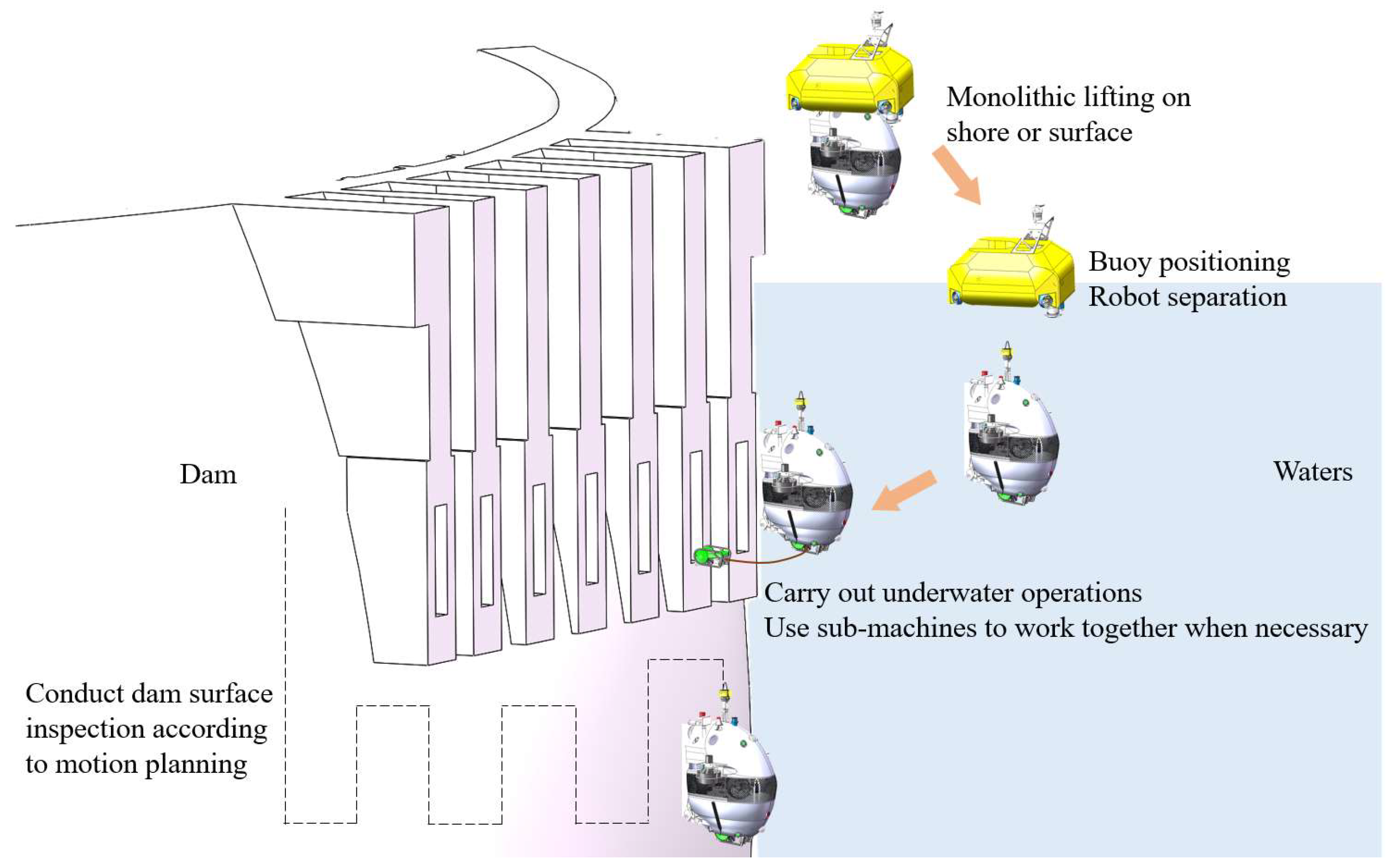
The vehicle operation process consists of deployment, diving, dam surface inspection, dredging, and recovery. As shown in Figure 6, the power buoy and vehicle are initially deployed together. After disconnecting from the buoy, the vehicle descends to the target dam surface and begins the planned inspection route. If certain areas are inaccessible, the sub-unit is deployed for further investigation. In cases of sediment buildup, the vehicle performs dredging to clear the silt. Finally, the vehicle collaborates with the propulsion system and umbilical cable for recovery.

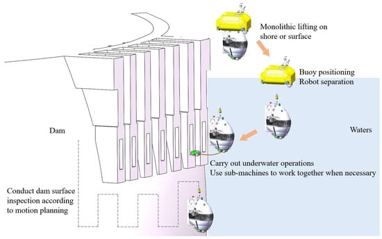
Figure 6. The process of the vehicle working underwater.

3. Hydrodynamic Simulation

3.1. The Principle of CFD Calculation

The law of conservation of momentum is a fundamental principle that must be followed in all flow problems. Within the target fluid system, the rate of change in fluid momentum over time equals the sum of external forces acting on the fluid during that time. The mathematical formulation of this principle is represented by the Navier–Stokes (N-S) equations, which are expressed as follows:

$$\rho \left({\displaystyle \frac{\partial u}{\partial t}}+u{\displaystyle \frac{\partial u}{\partial x}}\right)=f_x-{\displaystyle \frac{\partial p}{\partial x}}+div\left(grad \mu u\right)$$

(4)

$$\rho \left({\displaystyle \frac{\partial u}{\partial t}}+u{\displaystyle \frac{\partial v}{\partial y}}\right)=f_y-{\displaystyle \frac{\partial p}{\partial y}}+div\left(grad \mu v\right)$$

(5)

$$\rho \left({\displaystyle \frac{\partial u}{\partial t}}+u{\displaystyle \frac{\partial w}{\partial z}}\right)=f_z-{\displaystyle \frac{\partial p}{\partial z}}+div\left(grad \mu w\right)$$

(6)

Here, u, v, and w represent the fluid’s velocity components in the x, y, and z directions at time t at the point (x, y, z), respectively; ρ denotes the fluid density; p represents pressure; f is the external force acting on the fluid; and μ is the dynamic viscosity.

The principle of mass conservation applies to all fluid flow problems and is expressed as follows:

$$I{n}_{Mass/Time}=Ou{t}_{Mass/Time}$$

(7)

For an incompressible fluid, the above equation simplifies to

$${\displaystyle \frac{\partial u_i}{\partial x_i}}=0$$

(8)

3.2. Simulation of Direct Flight

Using a rectangular control domain as the computational area and referencing the relevant literature, as shown in Figure 7, the vehicle length is L. To ensure accurate simulation of hydrodynamic forces, the model is positioned such that its distance from the boundary in the x-direction is 6L, in the y-direction it is 4L, and in the z-direction it is 6L.

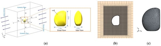
Figure 7. The setting of the calculation area and the division of grid: (a) the setting of the calculation area; (b) results of watershed grid division; (c) results of robot configuration surface meshing.

In the forward three-section working condition, the upstream x-axis boundary is set as the velocity inlet, while the downstream boundary is set as the pressure outlet; the remaining four faces are treated as symmetry planes, and the model surface is specified as a wall. For the transverse two-section condition, the y-axis surfaces are used as the velocity inlet and pressure outlet.

Based on the operational requirements, simulations were conducted to determine the straight-line resistance for the forward three-section and lateral two-section conditions. The results are presented in Table 1 and Figure 8. The direct navigation calculations indicate that the forward-flow surface experiences high pressure over a small area, resulting in substantial force and increased resistance when the streamlined configuration moves at high speed. In lateral flow, the larger incoming flow area causes a marked increase in the vehicle’s resistance.

Table 1. Simulation results for straight-line navigation resistance.

	Forward Three-Section/N	Lateral Two-Section/N
Simulation results for straight-line navigation resistance	117.818	300.517

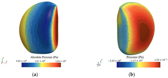
Figure 8. Surface pressure contour of the vehicle configuration: (a) forward three-section; (b) lateral two-section.

3.3. Hydrodynamic Experiments and Configuration Validation

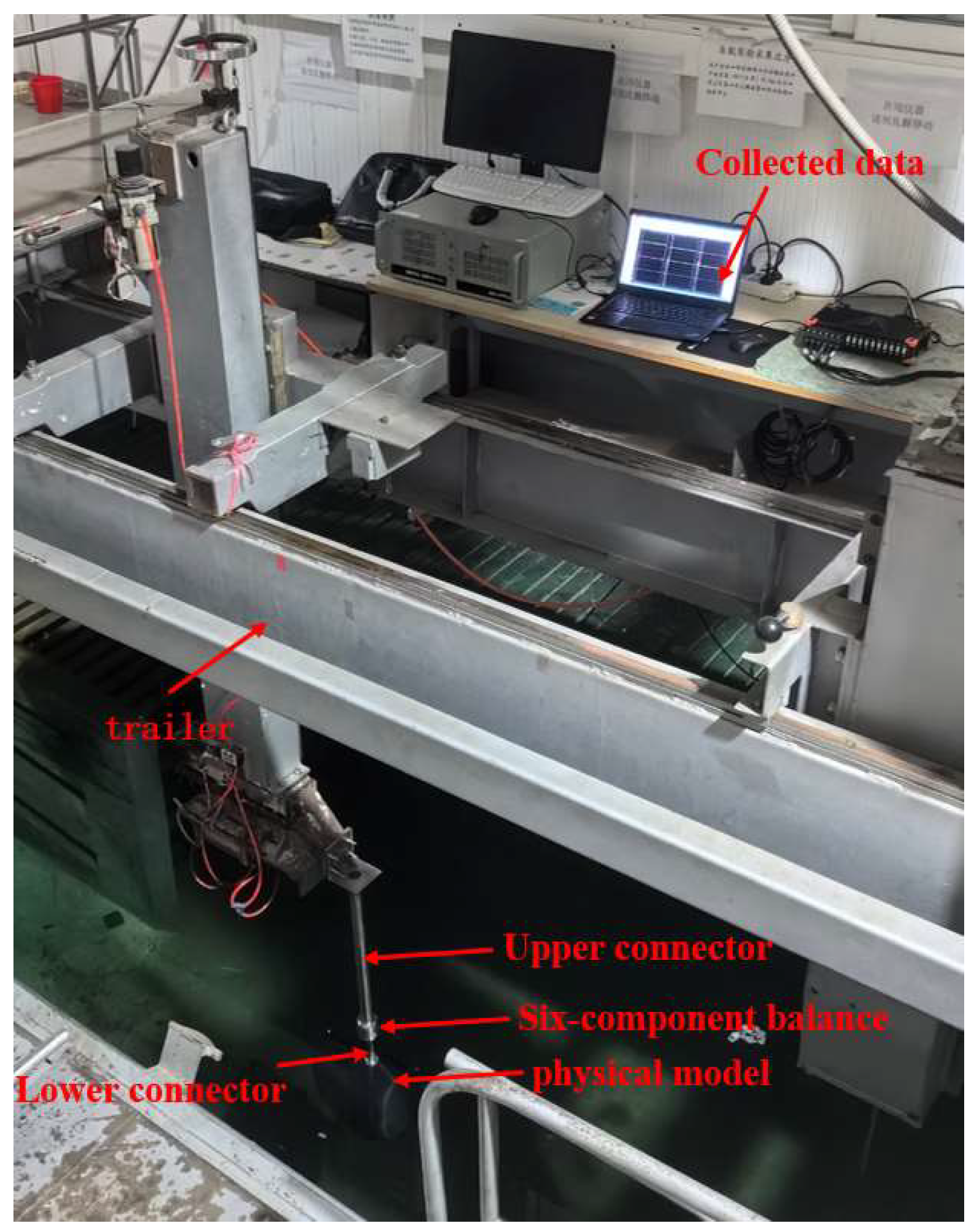
To validate the hydrodynamic calculations, a scaled physical model based on the streamlined configuration was constructed, and resistance measurements were taken under two operating conditions. The full-scale resistance was then determined using a conversion formula and compared with CFD results. The towing tests were conducted in the towing pool at Jiangsu University of Science and Technology, which measures 100 m in length, 5 m in width, and 3 m in depth. The physical model was constructed based on the Froude number scaling law, with a reduction ratio of 1:4.1, in accordance with previous experience and the constant Froude number formula (${\displaystyle \frac{v_s^2}{L_s}}={\displaystyle \frac{{1.5432}^2}{1.28}}={\displaystyle \frac{v_m^2}{L_m}}$). The main dimensions of the physical model are provided in Table 2. Data collection was performed using Dewesoft software, and the assembly test site is shown in Figure 9.

Table 2. Main scale of physical model of vehicle.

Model Scale	Value
long	0.312 m
wide	0.211 m
high	0.400 m
volume	0.244 m
Surface area	0.316 m

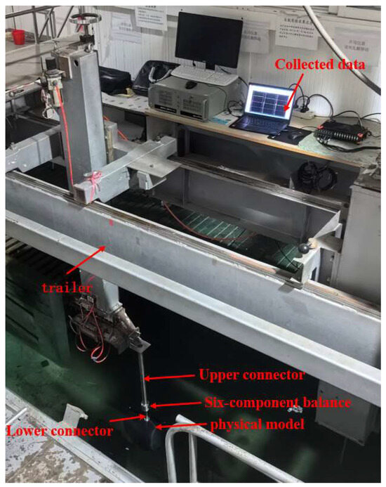
Figure 9. The assembly test site.

Three trailing tests, each lasting over 30 s, were conducted for two conditions, namely forward at 0.76 m/s and lateral at 0.51 m/s, with the average value taken for each. To account for the impact of the dead weight of the upper and lower connectors and the six-component balance on the results, a no-load test was first performed using only these two components. The final physical model test results were obtained by subtracting the no-load values from the measurements under the two working conditions.

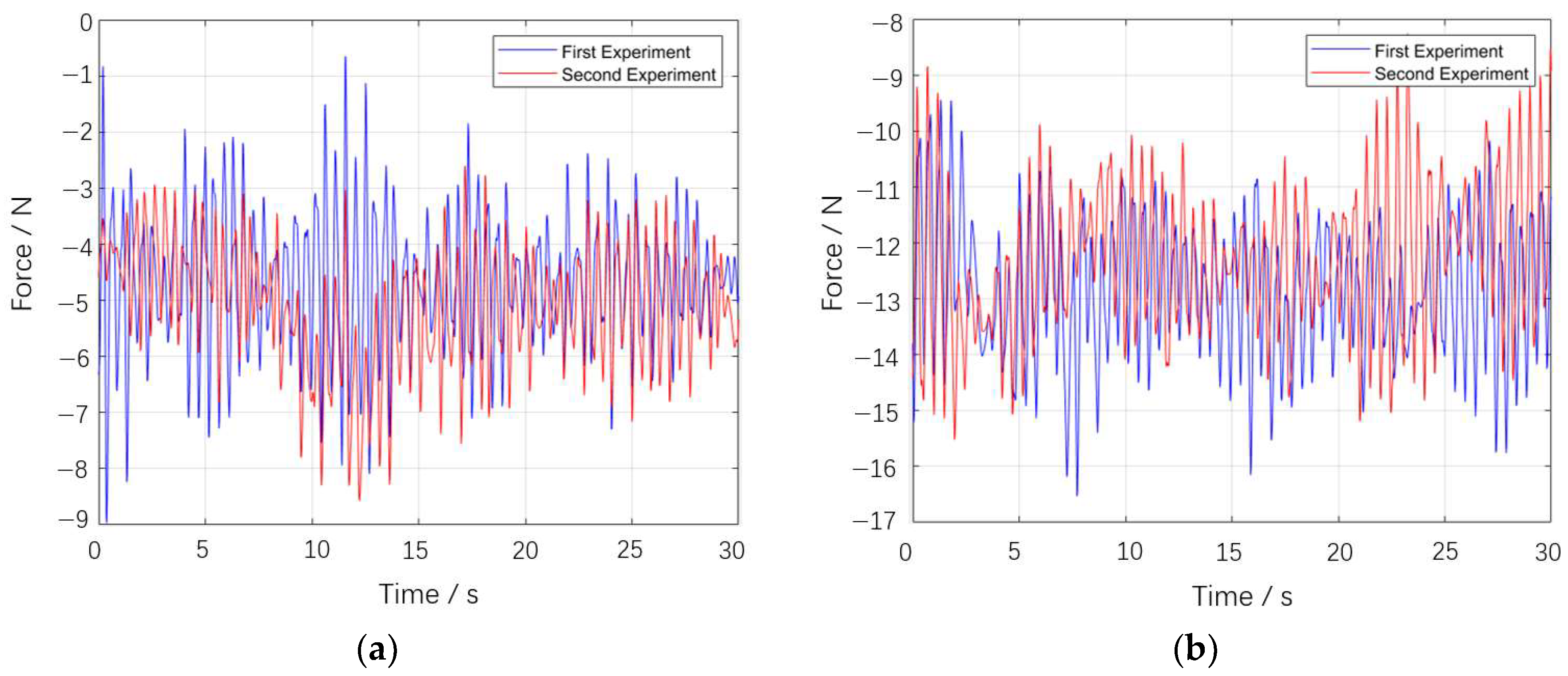
As shown in Figure 10, test results with significant errors were excluded, and the remaining data were averaged. The approximate resistance of the model under the two working conditions was then obtained by subtracting the no-load resistance from the total resistance. The calculation results are presented in Table 3.

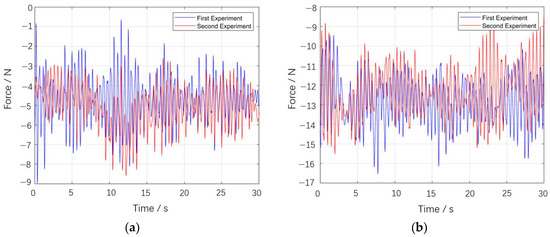
Figure 10. Comparison of force results of two tests: (a) forward 0.76 m/s; (b) lateral 0.51 m/s.

Table 3. Calculation results of four groups of experiments.

	Forward 0.76 M/S		Lateral 0.51 M/S
Number of Trials	Integral Resistance	No-Load Resistance	Integral Resistance	No-Load Resistance
1	−4.162 N	−2.181 N	−12.742 N	−0.721 N
2	−4.205 N	−2.156 N	−12.463 N	−0.723 N
3	−4.251 N	−2.147 N	−12.065 N	−0.724 N
Mean value	−4.206 N	−2.161 N	−12.423 N	−0.723 N
Difference between overall and no-load resistance	−2.044 N		−11.700 N

From the above, the forward drag force of the physical model under standard operating conditions is 2.044 N, which was then used for model drag conversion. The model design parameters are shown in Table 4.

Table 4. Model design parameters.

Argument	Date
The length of the physical model $L_m$	0.313 m
The surface area of the physical model $S_m$	0.316 m2
The speed of the physical model $V_m$	0.760 m/s
The drag force of the physical model $R_m$	2.044 N
The length of the actual size configuratio $L_s$	1.280 m
The surface area of the actual size configuratio $S_s$	5.314 m2
The speed of the actual size configuration $V_s$	1.543 m/s
Scaling ratio $\alpha$	4.1

The resistance of the scaled physical model was converted to correspond to the full-scale configuration, with the final results presented in Table 5. The calculations show that the error between the resistance conversion result and the CFD calculation under the forward three-section condition is 4.98%, while the error for the lateral two-section condition is 3.65%. Both results fall within the acceptable error range, confirming the accuracy of the CFD calculation method.

Table 5. The results of resistance conversion.

	Forward 0.76 m/s	Lateral 0.51 m/s
Result of resistance conversion	123.690 N	311.492 N
Result of CFD simulation	117.818 N	300.517 N
Error	4.98%	3.65%

3.4. Stability Analysis

The stability of an underwater vehicle includes both static and dynamic stability. High stability enhances the vehicle’s maneuverability.

3.4.1. Simulation of Variable Angle of Attack and Variable Angle of Drift

At three throttling speeds, the vertical and horizontal hydrodynamic forces were calculated using CFD within the range of [−10°,10°] for both the angle of attack α and the drift angle β. The torque distribution of the hydrodynamic center along the x-axis was analyzed to identify the maneuverability center. Figure 11 illustrates the definitions of the attack angle α and drift angle β.

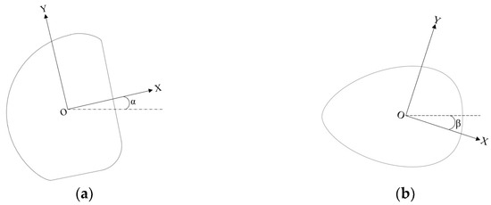
Figure 11. Definition of angle of attack and angle of drift: (a) attack angle α; (b) drift angle β.

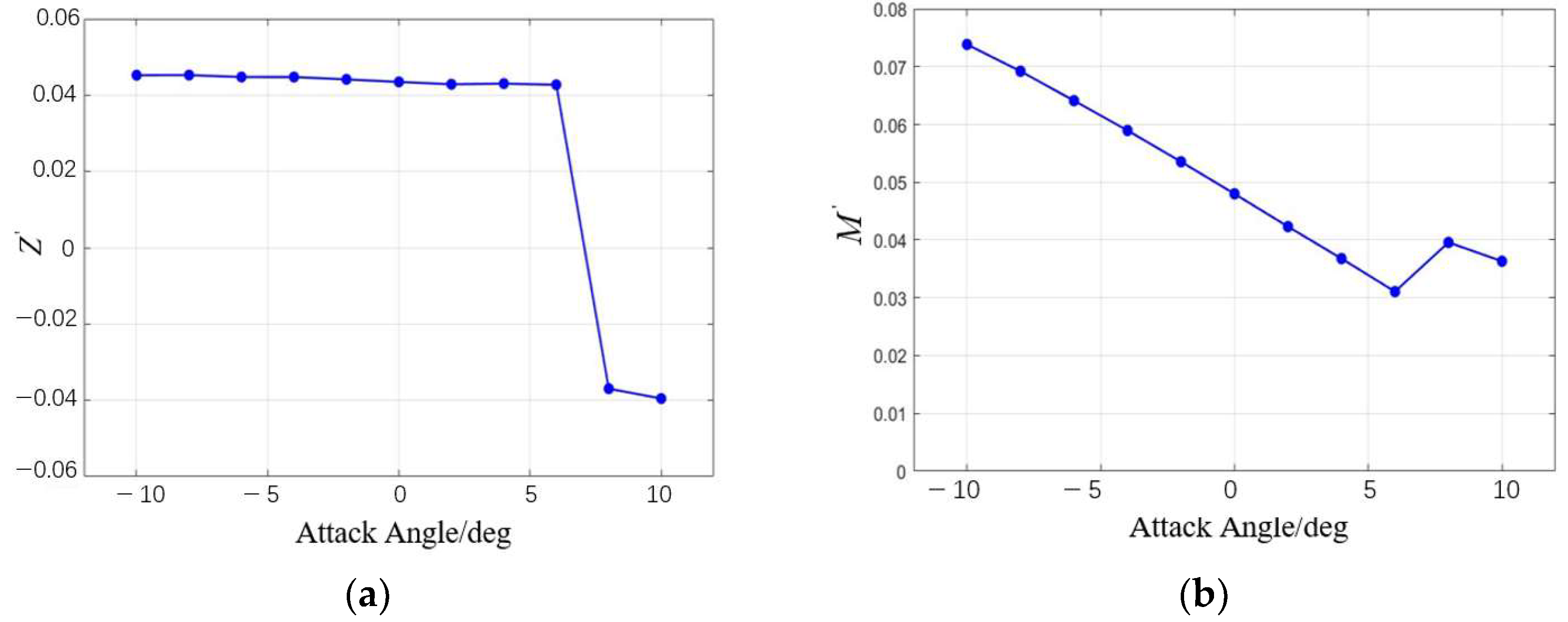
The results obtained were dimensionless, leading to the determination of the lift coefficient and pitching moment coefficient for varying angles of attack, as shown in Figure 12. Within the range of [−10°, 6°], both the lift force and pitching moment exhibit good linearity, with instability observed beyond 6°. Fitting a linear relationship for the range [−10°, 6°] yields position derivatives of $Z_w^{\prime }=-0.0002$ and $M_w^{’}=-0.0027$.

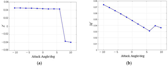
Figure 12. The variation in the lift coefficient $Z_w^{’}$ and pitching moment coefficient $M_w^{’}$ with the angle of attack: (a) the variation in the lift coefficient $Z_w^{’}$ with the angle of attack; (b) the variation in the pitching moment coefficient $M_w^{’}$ with the angle of attack.

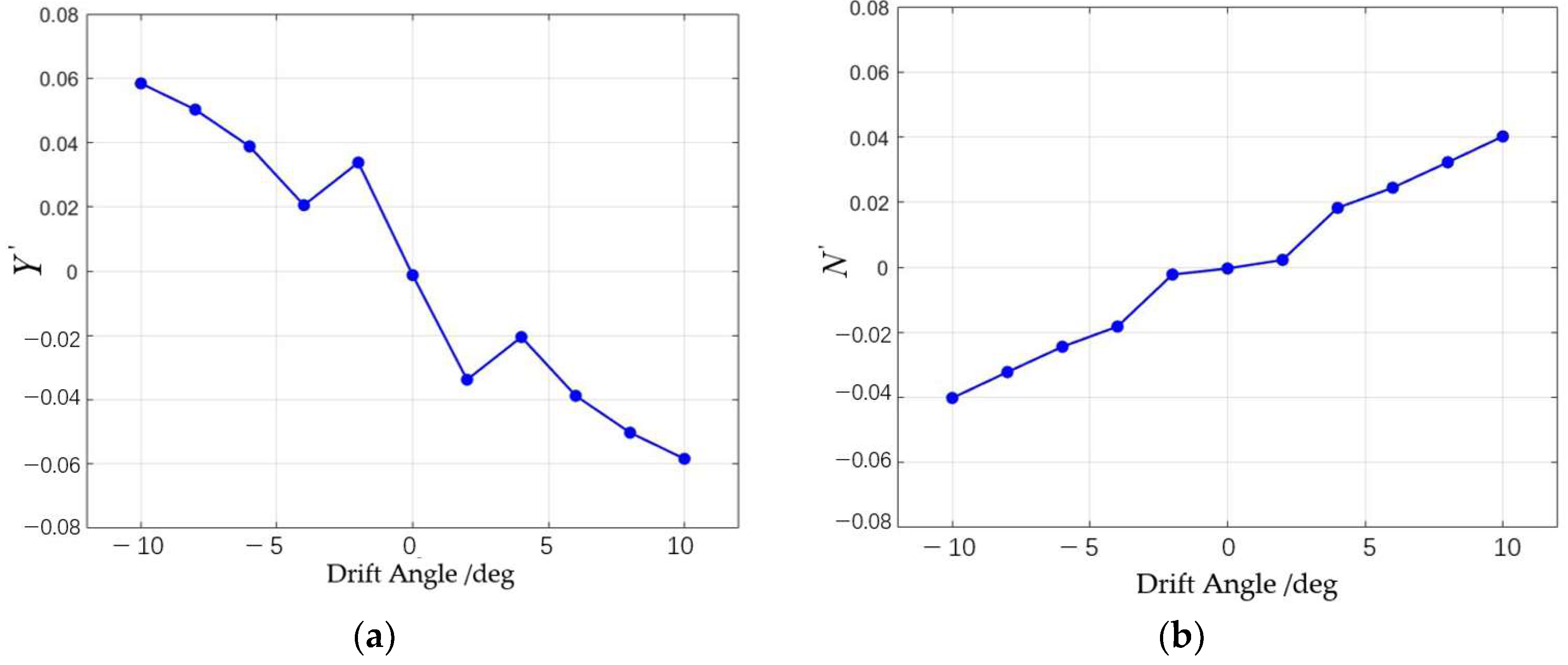
Similarly, the lateral force coefficient and yaw moment coefficient for varying drift angles were dimensionless, with the final results shown in Figure 13. The vehicle’s lateral force coefficient exhibits instability between −2° and 2°, but overall, the relationship is approximately linear. Linear fitting of the data gives position derivatives of $Y_v^{’}=-0.0062$ and $N_v^{’}=0.0040$.

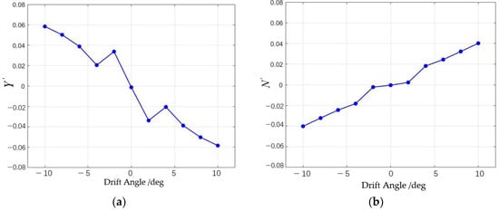
Figure 13. The variation in the lateral force coefficient $Y_v^{’}$ and yaw moment coefficient $N_v^{’}$ with the drift angle: (a) the variation in the lateral force coefficient $Y_v^{’}$ with the angle of attack; (b) the variation in the yaw moment coefficient $N_v^{’}$ with the angle of attack.

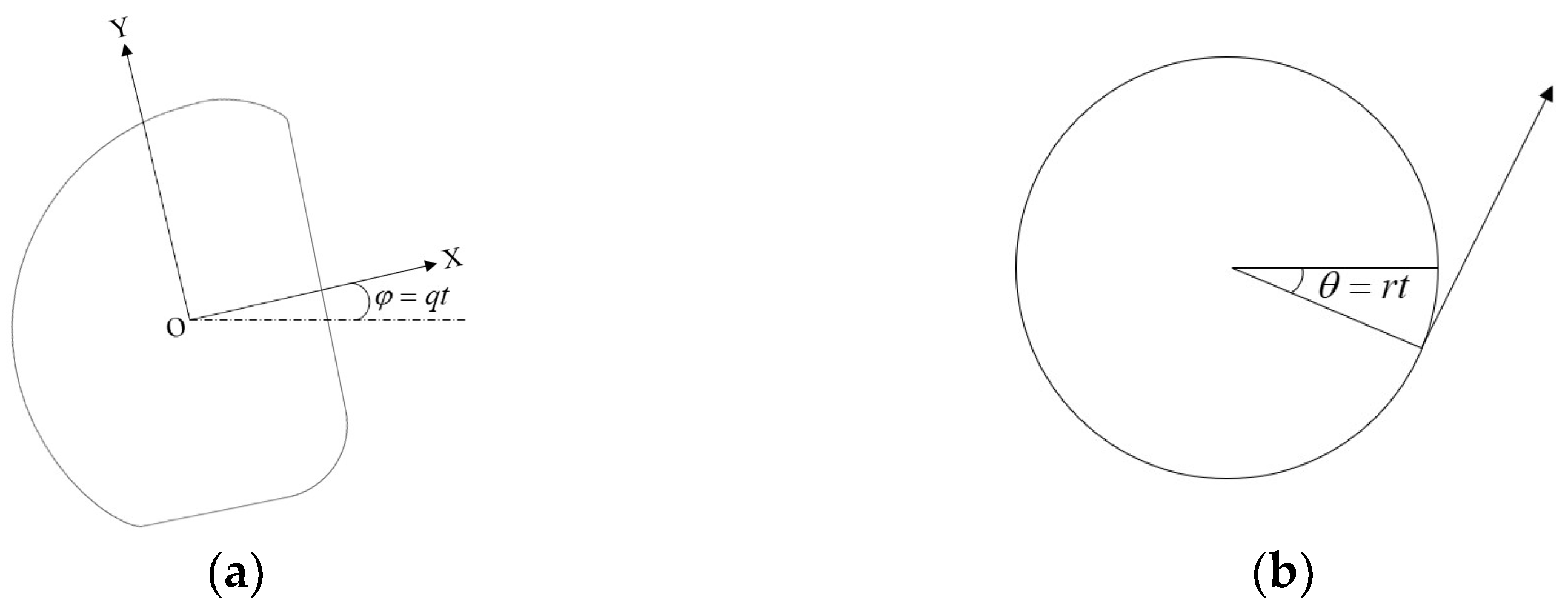
3.4.2. Simulation of Pitch and Turn Motion

The changes in the longitudinal angular velocity $q={\displaystyle \frac{d\phi }{dt}}$ and turning angle $r={\displaystyle \frac{d\theta }{dt}}$ of the hydrodynamic center impact the course stability of the underwater vehicle in both the vertical and horizontal planes. To evaluate this, the hydrodynamic derivatives $M_q$, $Z_q$, $Y_r$, and $N_r$ must be calculated. The angular velocity was varied within the interval [1 deg/s, 3 deg/s] in steps of 0.5 deg/s, and the pitching and rotational motion performance was simulated using the rotating coordinate system method, as shown in Figure 14.

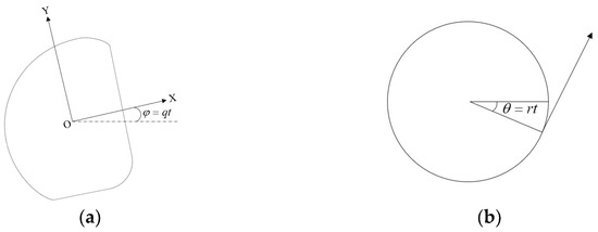
Figure 14. Definition of pitching motion and turning motion: (a) pitching motion, (b) turning motion.

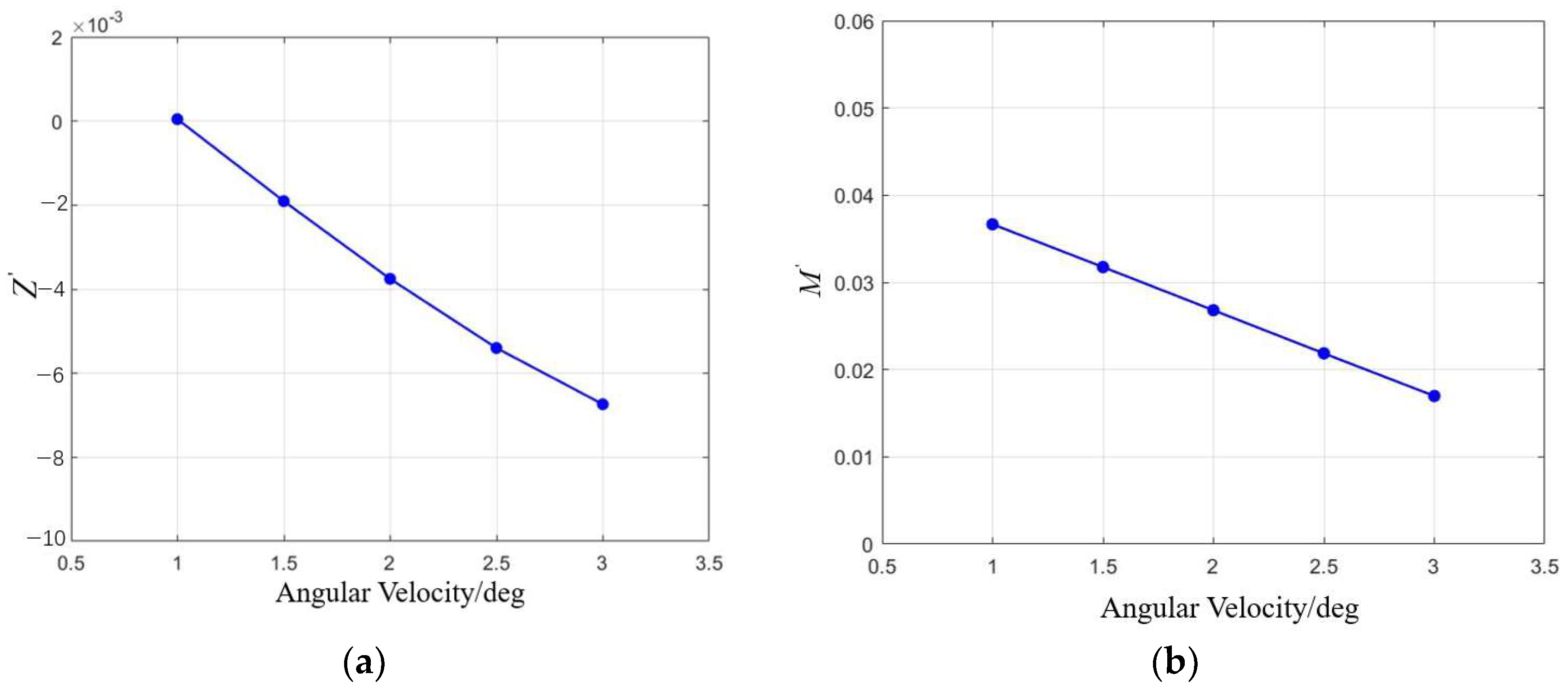
The obtained data were dimensionless, and the corresponding hydrodynamic coefficients were calculated, as shown in Figure 15. Both the lift coefficient and pitching moment coefficient exhibited an approximately linear relationship with angular velocity. A linear fit was applied, yielding $Z_q^{’}=-0.0034$ and $M_q^{’}=-0.0099$.

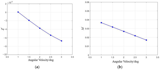
Figure 15. The variation in the lift coefficient $Z_q^{’}$ and pitching moment coefficient $M_q^{’}$ with pitch angular velocity: (a) the variation in the lift coefficient $Z_q^{’}$ with pitch angular velocity; (b) the variation in the pitching moment coefficient $M_q^{’}$ with pitch angular velocity.

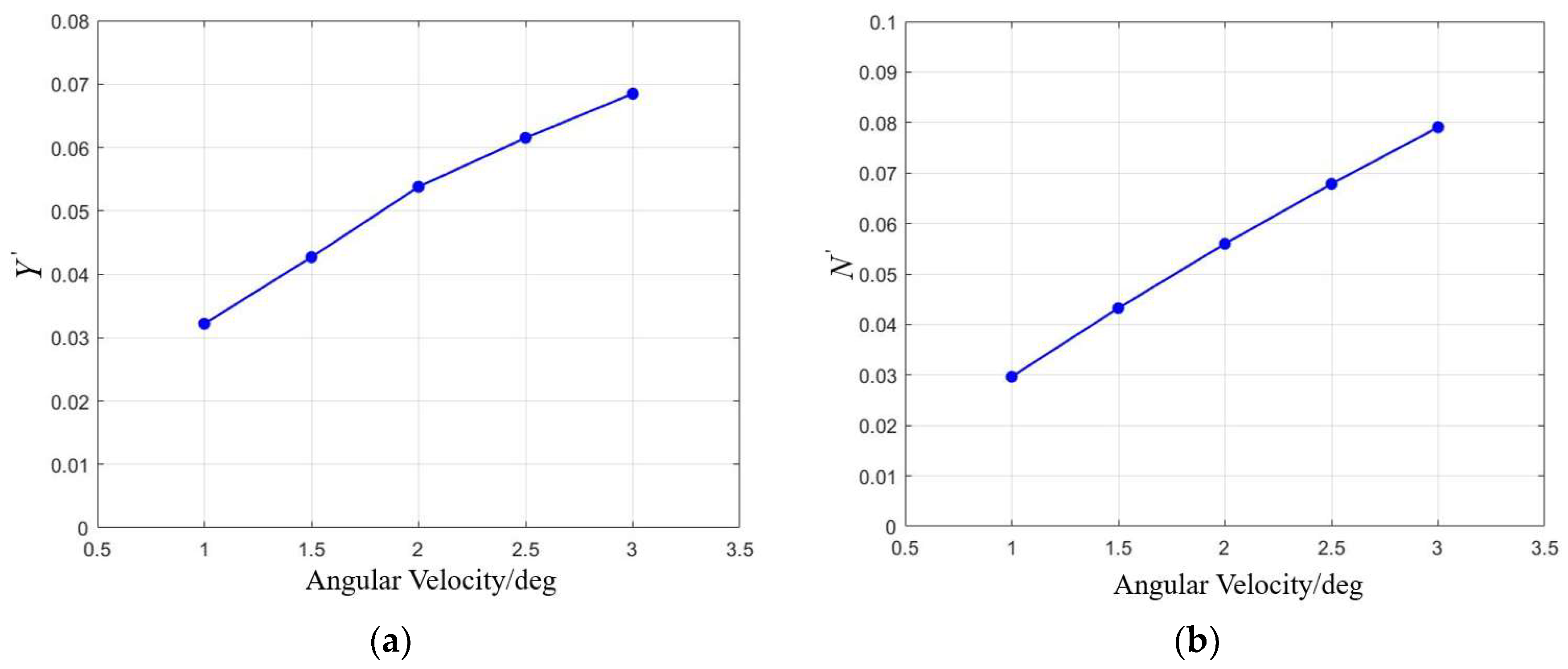
Similarly, as shown in Figure 16, the lateral force coefficient and yaw moment coefficient exhibit an approximately linear relationship with the rotational angular velocity. Fitting a linear model yields $Y_r^{’}=0.0181$ and $N_r^{’}=0.0247$.

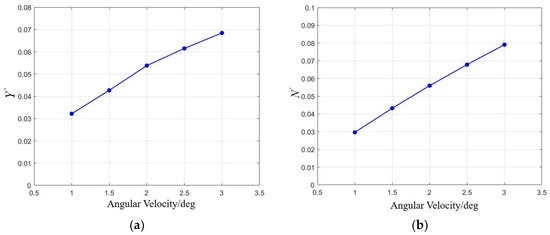
Figure 16. The variation in the lateral force coefficient $Y_r^{’}$ and yaw moment coefficient $N_r^{’}$ with pitch angular velocity: (a) the variation in the lateral force coefficient $Y_r^{’}$ with pitch angular velocity; (b) the variation in the yaw moment coefficient $N_r^{’}$ with pitch angular velocity.

3.4.3. Stability Assessment

This section evaluates the stability of underwater vehicles by considering both static and dynamic criteria.

Static stability focuses on the change in a single parameter during constant motion, addressing only the initial motion response after the removal of external disturbances. The vertical and horizontal stability of the vehicle is determined by the sign of the dimensionless hydrodynamic center lever:

$${l^{\prime }}_{\alpha }=-{\displaystyle \frac{{M^{\prime }}_w}{{Z^{\prime }}_w}}, {l^{\prime }}_{\beta }={\displaystyle \frac{{N^{\prime }}_v}{{Y^{\prime }}_v}}$$

(9)

The stability improves as the value of the dimensionless hydrodynamic center lever decreases. When ${l^{\prime }}_{\alpha }<0$, the angle of attack α is considered statically stable. Conversely, if ${l^{\prime }}_{\alpha }>0$, the system is unstable. This method of determination is also applicable to ${l^{\prime }}_{\beta }$.

If the relationship between the static instability coefficient in the vertical plane ${l^{\prime }}_{\alpha }$ and the dimensionless pitching lever ${l^{\prime }}_q$ is satisfied such that

$${l^{\prime }}_{\alpha }<{l^{\prime }}_q,$$

(10)

this indicates that dynamic stability can be achieved at any speed in the vertical plane, where the dimensionless hydrodynamic center lever ${l^{\prime }}_{\alpha }=-{\displaystyle \frac{{M^{\prime }}_w}{{M^{\prime }}_q}}$ and the dimensionless relative damping lever ${l^{\prime }}_q=-{\displaystyle \frac{{M^{\prime }}_q}{(m^{\prime }+{Z^{\prime }}_q)}}$.

Stability in the horizontal plane is governed by similar criteria:

$$C_H={N^{\prime }}_r{Y_v}^{\prime }+{N^{\prime }}_v(m^{\prime }-{Y^{\prime }}_r)>0$$

(11)

This indicates that the system possesses dynamic stability in the horizontal plane. Therein, $m^{’}={\displaystyle \frac{m}{\frac{1}{2}\rho L^3}}$.

Based on the above calculations, as shown in Table 6, it can be concluded that the vehicle configuration exhibits static stability in the vertical plane within the range of [−10°, 6°], as both the lift coefficient and pitching moment coefficient become unstable when the angle of attack exceeds 6°. Additionally, the configuration shows dynamic stability in the vertical plane but lacks dynamic stability in the horizontal plane.

Table 6. Stability analysis results.

	Static Stability			Dynamic Stability
	Argument	Result	Determining Static Stability	Argument	Result	Determining Dynamic Stability
Vertical Plane	${l^{\prime }}_{\alpha }$	−13.5	Yes	${l^{\prime }}_{\alpha }$	−0.272	Yes
				${l^{\prime }}_q$	0.0617
Horizontal Plane	${l^{\prime }}_{\beta }$	−0.645	Yes	$C_H$	−2.805	No

4. Optimization of Configuration

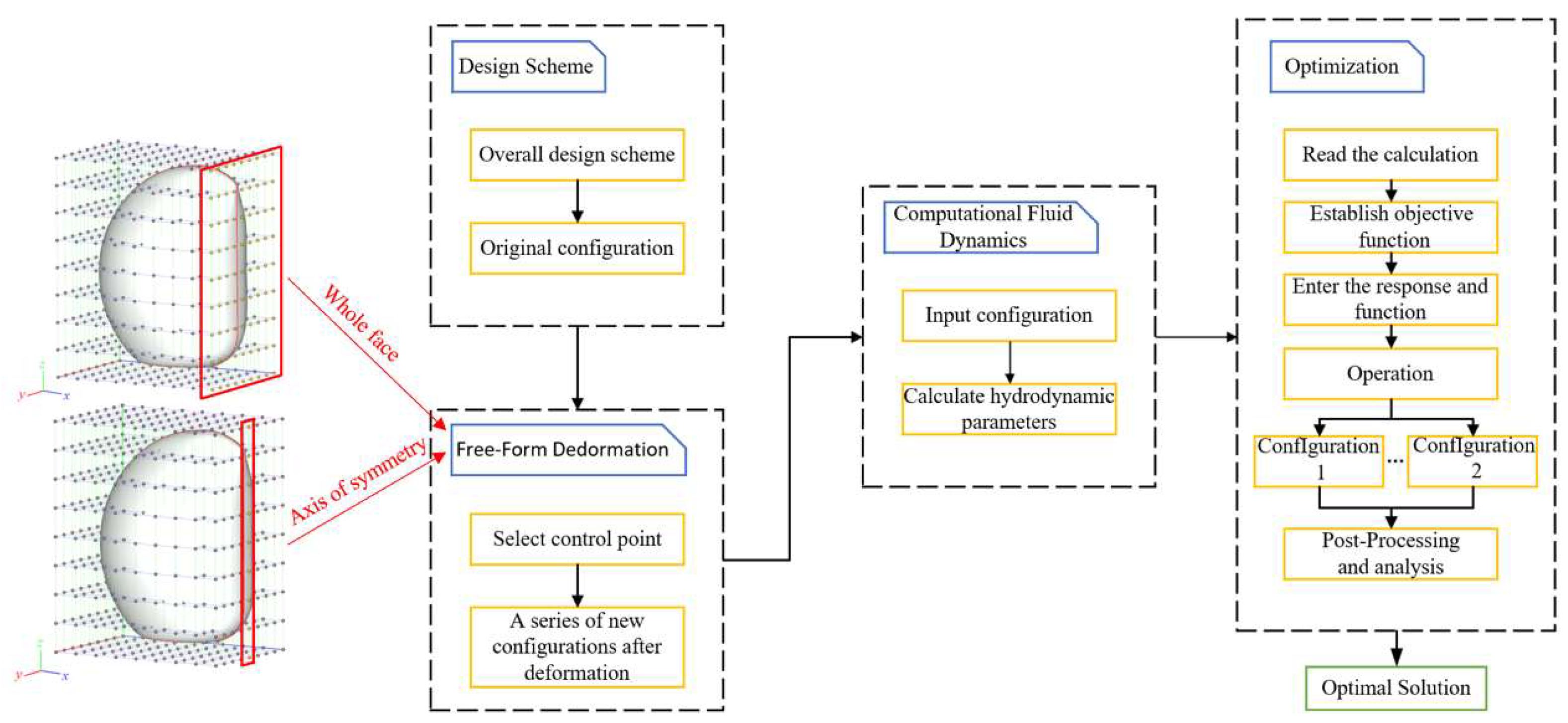
The vehicle configuration optimization process (Figure 17) utilizes free deformation technology to modify the original design, establishing an optimization objective function. This process is divided into four steps: design, deformation, simulation, and optimization. CAESES software was used for free deformation, with the vehicle configuration deformation grid set to 1.5 m × 1 m × 1.8 m, divided into eight equal sections.

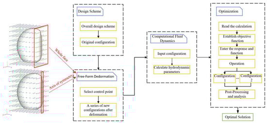
Figure 17. Flowchart for optimizing vehicle configuration.

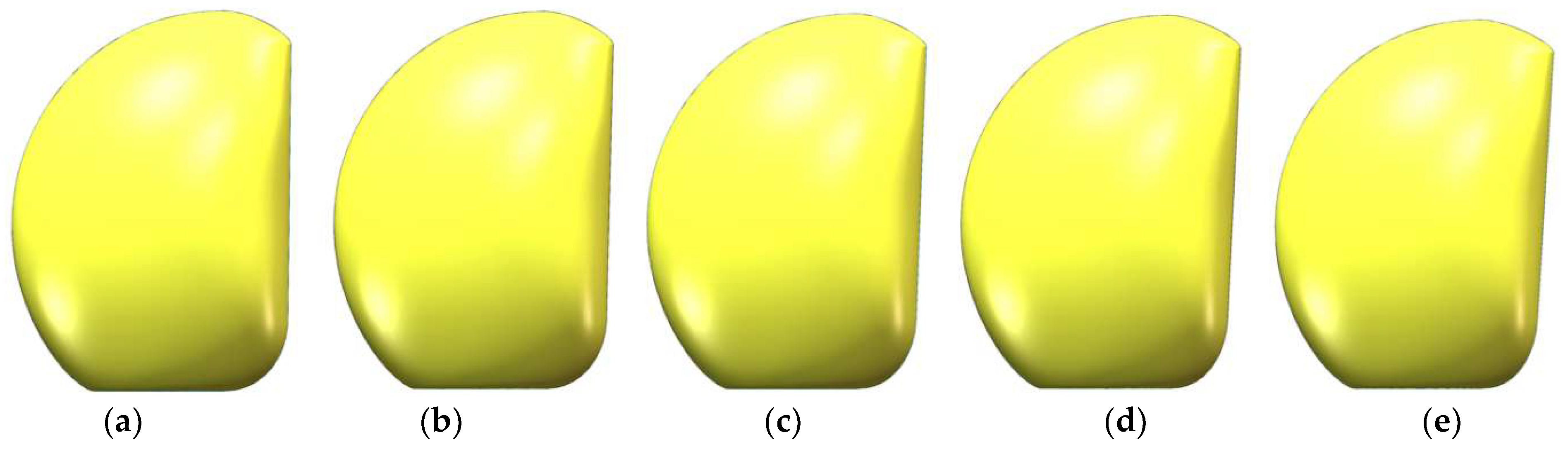
The deformation size corresponds to the change in control points, with the influence diminishing as the control points move away from the surface. Based on the grid distribution, two deformation operations were performed (Figure 18, Figure 19 and Figure 20), as follows:

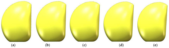
Figure 18. Surface tilt range from −1° to −5° (front view): (a) tilt −1°; (b) tilt −2°; (c) tilt −3°; (d) tilt −4°; (e) tilt −5°.

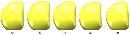
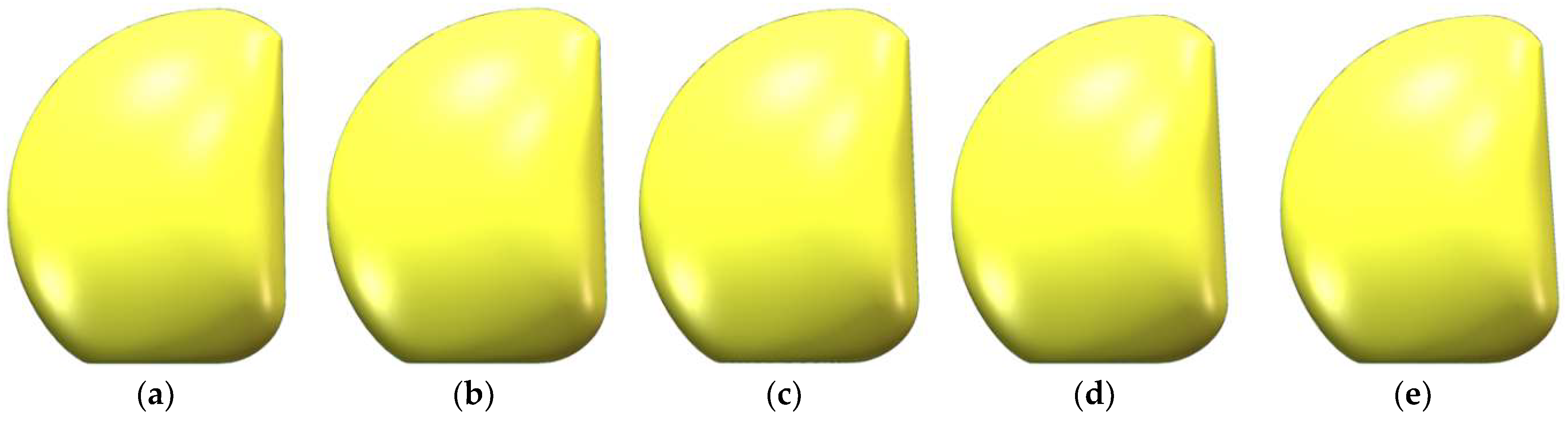
Figure 19. Surface tilt range from 1° to 5° (front view): (a) tilt 1°; (b) tilt 2°; (c) tilt 3°; (d) tilt 4°; (e) tilt 5°.

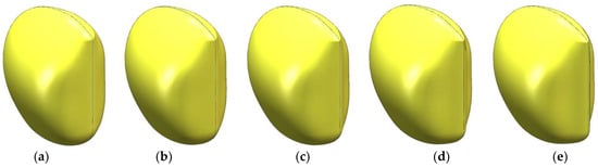
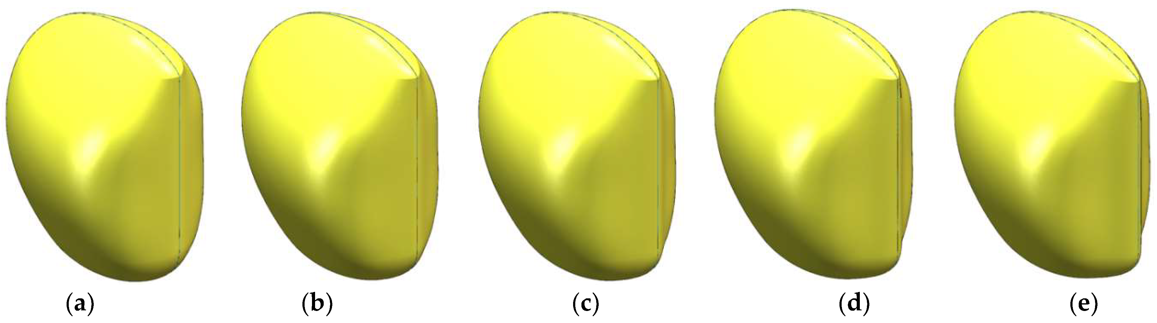
Figure 20. Surface stretch of 0.05 m to 0.25 m (isometric view): (a) stretch of 0.05 m, (b) stretch of 0.1 m, (c) stretch of 0.15 m, (d) stretch of 0.2 m, and (e) stretch of 0.25 m.

• Control points along the vehicle’s working face in the x-direction were selected, and their longitudinal tilt angle was adjusted within a range of [−5°, 5°], with a step size of 1°.
• The symmetry axis of the vehicle’s working face was selected, and its stretching parameters along the x-axis (forward direction) were modified within a range of [0.05 m, 0.25 m], with a step size of 0.05 m.

To optimize the vehicle’s performance, multiple configurations are generated through local deformation, and the one with the best overall performance is selected. The optimization is constrained by a drainage volume variation of ≤2%, with resistance and stability as the primary objectives. Due to the limited propeller power caused by the umbilical cable, the weight of resistance is relatively low, while the weight of stability is higher. The optimization function is defined as follows:

$$\min F\left(X\right)={\displaystyle \frac{1}{3}}{\xi }_1+{\displaystyle \frac{2}{3}}({\xi }_2+{\xi }_3),$$

(12)

$${\xi }_1={\displaystyle \frac{1}{2}}{\displaystyle \frac{F_m-F_p}{F_p}}+{\displaystyle \frac{1}{2}}{\displaystyle \frac{F_n-F_t}{F_t}}$$

(13)

$${\xi }_2={\xi }_{x2}+{\xi }_{y2}$$

(14)

$${\xi }_{x2}=\left\{\begin{array}{l}0,\hspace{1em}{l}_{\alpha }^{’}<0\\ 0.01,l_{\alpha }^{’}\ge 0\end{array}\right., {\xi }_{y2}=\left\{\begin{array}{l}0,\hspace{1em}{l}_{\beta }^{’}<0\\ 0.01,l_{\beta }^{’}\ge 0\end{array}\right.$$

(15)

$${\xi }_3={\xi }_{x3}+{\xi }_{y3}$$

(16)

$${\xi }_{x3}=\left\{\begin{array}{l}0,\hspace{1em}{l}_{\alpha }^{’}<l_q^{’}\\ 0.01,l_{\alpha }^{’}\ge l_q^{’}\end{array}\right., {\xi }_{y3}={\displaystyle \frac{C_H-C_0}{C_0}}$$

(17)

$$s.t\left|{\displaystyle \frac{V_m-V}{V}}\right|\le 2\%$$

(18)

In these equations, $F_m$ and $F_p$ represent the drag forces of the deformed and original configurations, respectively, under the forward three-segment condition. $F_n$ and $F_t$ represent the drag forces of the deformed and original configurations, respectively, under the lateral two-segment condition. ${\xi }_{x2}$ is the vertical plane static stability criterion, ${\xi }_{y2}$ is the horizontal plane static stability criterion, ${\xi }_{x3}$ is the vertical plane dynamic stability criterion, and ${\xi }_{y3}$ is the horizontal plane dynamic stability criterion. $C_H$ and $C_0$ are the horizontal plane stability parameters for the deformed and original configurations, respectively. $V_m$ represents the volume of the deformed configuration, and $V$ represents the volume of the original configuration.

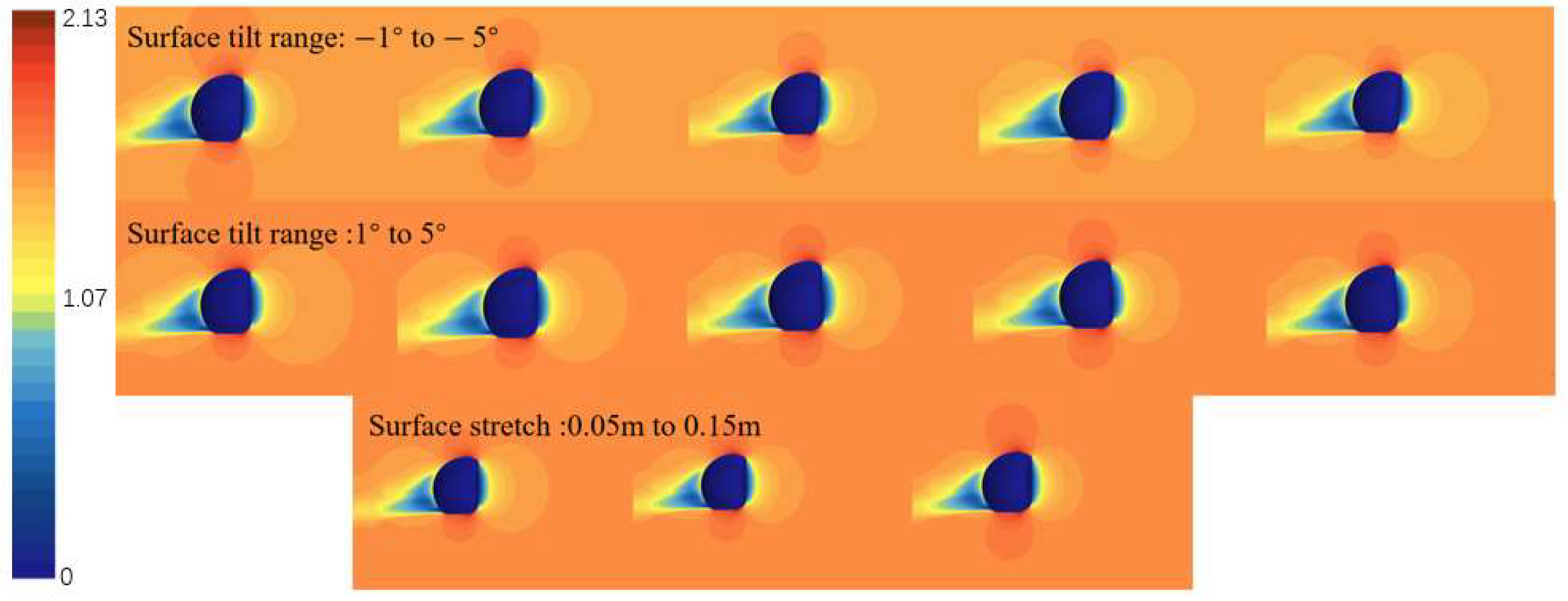
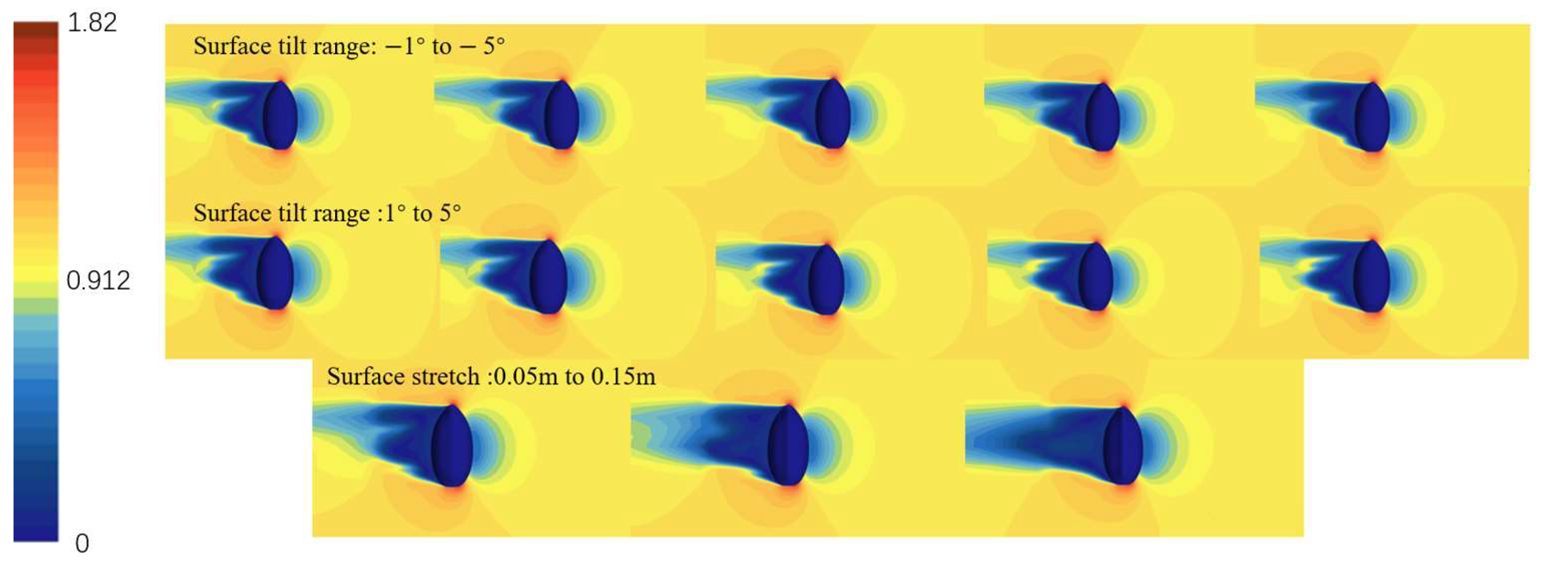
The deformation configurations of 0.20 m and 0.25 m do not satisfy the optimization constraints and are therefore excluded. To investigate the hydrodynamic behavior of the vehicle under forward three-knot and lateral two-knot inflows, velocity contour plots for various deformation configurations were generated through steady-state simulations. The results are presented in Figure 21, Figure 22, Figure 23 and Figure 24.

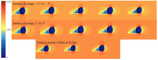
Figure 21. Velocity contour plots of forward 3-knot flow (front view).

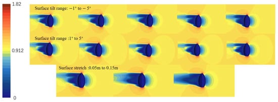
Figure 22. Velocity contour plots of lateral 2-knot flow (side view).

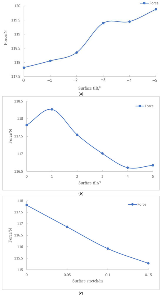
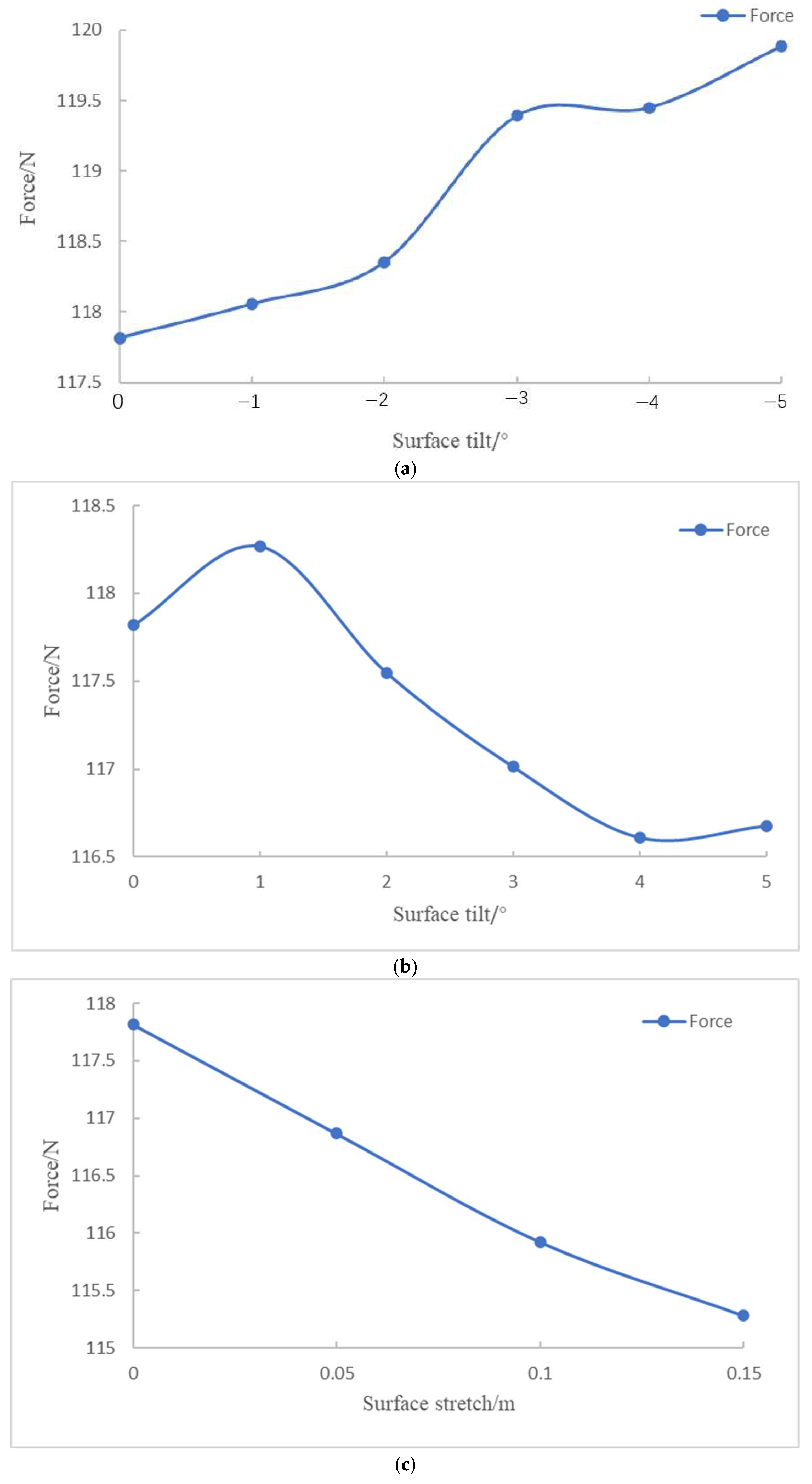
Figure 23. Variation in resistance under forward 3-knot flow: (a) surface tilt range of −1° to −5°; (b) surface tilt range of 1° to 5°; (c) surface stretch of 0.05 m to 0.15 m.

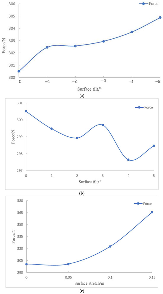
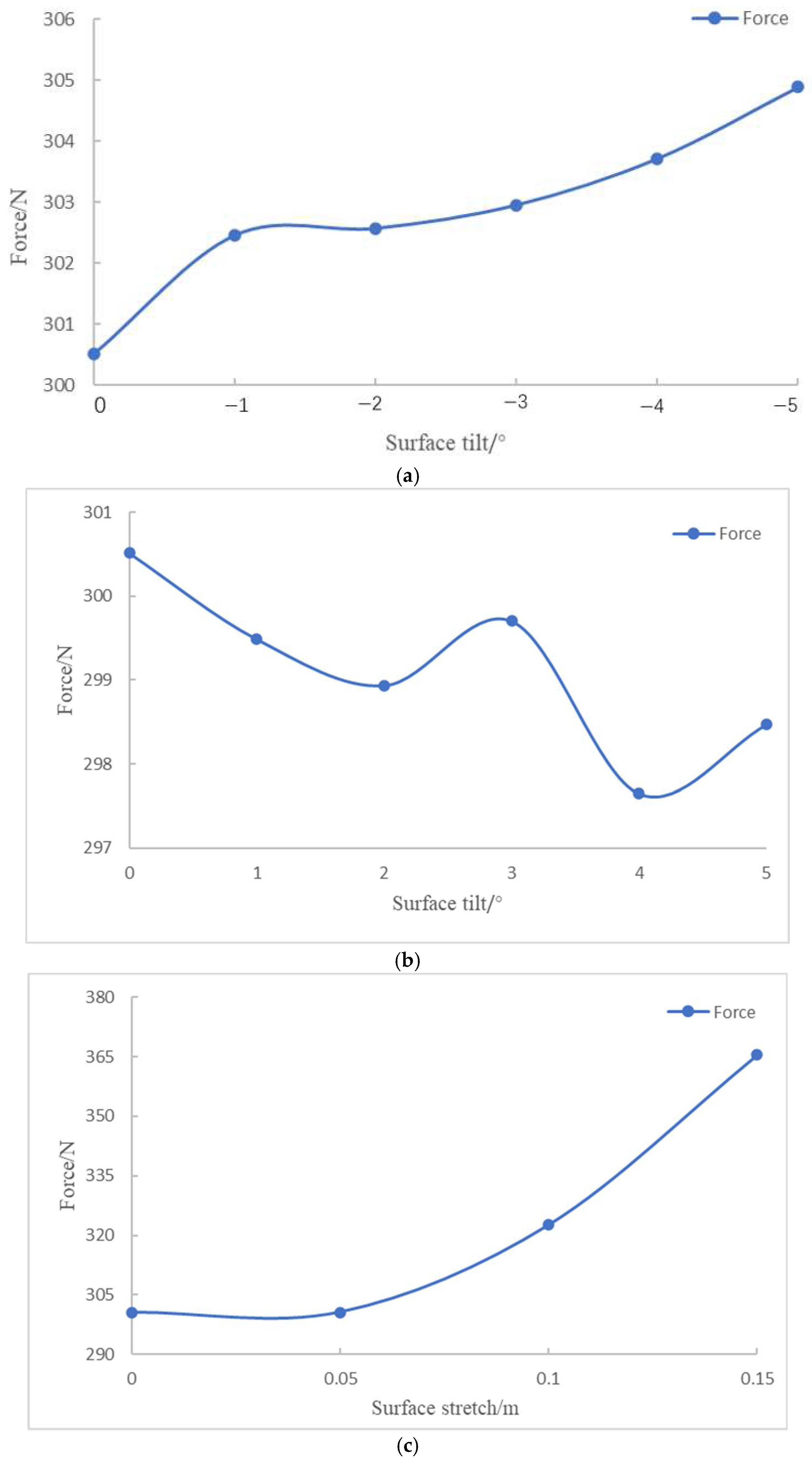
Figure 24. Variation in resistance under lateral 2-knot flow: (a) surface tilt range of −1° to −5°; (b) surface tilt range of 1° to 5°; (c) surface stretch of 0.05 m to 0.15 m.

The static stability of the series configuration was evaluated through simulations involving variable angles of attack and drift. As shown in Table 7, the results indicate that changes in the tilt or stretch of the oncoming plane have minimal impact on the static stability of both the vertical and horizontal planes, with the configuration remaining stable within a tilt range of [−10°, 6°]. Increasing the bottom indentation and top outward expansion improves the horizontal static stability. Dynamic stability is then assessed through simulations of pitching and rotating motions. It is observed that variations in the oncoming surface significantly affect the dynamic stability in the horizontal plane. Specifically, the C_H coefficient decreases as the tilt angle increases, while it increases with the stretching of the oncoming surface. However, all configurations lack horizontal dynamic stability. The vertical dynamic stability remains largely unaffected by these changes, ensuring stability in the vertical plane.

Table 7. Evaluation of static and dynamic stability coefficients for different configurations.

Serial Number	Configuration	Static Stability		Dynamic Stability			$\mathit{F}\left(\mathit{X}\right)$
		${\mathit{l}}_{\mathit{\alpha }}^{’}$	${\mathit{l}}_{\mathit{\beta }}^{’}$	${\mathit{C}}_{\mathit{H}}$	${\mathit{l}}_{\mathit{\alpha }}^{’}$	${\mathit{l}}_{\mathit{q}}^{’}$
1	Tilt −5°	−13.5	−0.661	−7.247	−0.529	0.0315	1.06125
2	Tilt −4°	−13.5	−0.656	−5.432	−0.479	0.0377	0.62862
3	Tilt −3°	−13.5	−0.652	−4.241	−0.434	0.0455	0.34517
4	Tilt −2°	−13.5	−0.648	−3.237	−0.361	0.0518	0.10444
5	Tilt −1°	−13.5	−0.645	−2.805	−0.275	0.0611	0.00117
6	Origin	−13.5	−0.645	−2.805	−0.272	0.0617	0
7	Tilt 1°	−13.5	−0.645	−2.805	−0.279	0.0610	0.00047
8	Tilt 2°	−13.5	−0.638	−3.169	−0.346	0.0523	0.08542
9	Tilt 3°	−13.5	−0.621	−4.180	−0.425	0.0461	0.32498
10	Tilt 4°	−13.5	−0.609	−5.015	−0.460	0.0384	0.52191
11	Tilt 5°	−13.5	−0.609	−6.522	−0.519	0.0319	0.88052
12	Stretch 0.05 m	−13.5	−0.627	−2.340	−0.265	0.0586	−0.11228
13	Stretch 0.10 m	−13.5	−0.635	−2.064	−0.253	0.0550	−0.1715
14	Stretch 0.15 m	−13.5	−0.655	−1.815	−0.240	0.0517	−0.21605

As shown in Table 8, the optimal configuration corresponds to a 0.15 m surface stretch deformation. Compared to the original design, this configuration results in a 2.15% reduction in forward resistance, a 21.62% increase in lateral resistance, and a 1.98% increase in volume. It exhibits good static stability and maintains vertical dynamic stability. While it lacks full horizontal dynamic stability, the horizontal stability improves from −2.805 to −1.815, indicating a notable enhancement in horizontal plane dynamic stability.

Table 8. Comparison of configuration parameters before and after optimization.

Argument	Original Configuration	Optimized Configuration	Rate of Change
Resistance in the forward 3-knots condition/N	117.818	115.282	−2.15%
Resistance in the lateral 2-knots condition/N	300.517	365.502	21.62%
Vertical static stability	−13.5	−13.5	-
Horizontal static stability	−0.645	−0.655	−1.55%
Vertical dynamic stability	yes	yse	-
Horizontal dynamic stability	−2.805	−1.815	35.29%

5. Conclusions

This paper addresses the demand for underwater dam defect detection by designing an overall layout and operational mode for a streamlined underwater robot and parameterizing the streamlined configuration. CFD methods were used to conduct a series of hydrodynamic simulations on the configuration, calculating relevant hydrodynamic coefficients and determining the stability of the configuration. A scaled physical model was built, and resistance data were collected through towing tests in a water tank. The full-scale drag was then calculated using a drag conversion formula, and the reliability of the CFD method was verified through comparison. A series of different configurations were generated using the free deformation method, and hydrodynamic simulations were performed for each. The drag and stability performance were used to establish an optimization objective function, which was optimized using a genetic algorithm. The main research findings of this paper are as follows:

1. In response to the specific requirements of underwater dam defect detection, a streamlined configuration inspired by the shape of a seahorse was designed, integrating the vehicle’s hydrodynamic performance and operational posture. This bionic design is particularly significant for the development of the ROV hover system.

2. A streamline model of the vehicle was developed to assess its hydrodynamic coefficients under various working conditions. The evaluation results show that, while the vehicle lacks horizontal dynamic stability, it maintains static stability in both the horizontal and vertical planes, as well as dynamic stability in the vertical plane.

3. The vehicle’s original configuration was optimized using free deformation technology. The optimization function, focused on resistance and stability, with a volume change constraint of ≤2%, was established. The optimized configuration resulted in a 2.152% reduction in forward resistance and a 35.29% improvement in horizontal dynamic stability (C_H).

References

- Benchimol, M.; Peres, C.A. Predicting local extinctions of Amazonian vertebrates in forest islands created by a mega dam. Biol. Conserv. 2015, 187, 61–72. [Google Scholar] [CrossRef]
- Carmignotto, A.P. Effects of damming on a small mammal assemblage in Central Brazilian Cerrado. Bol. Soc. Bras. Mastozool. 2019, 85, 63–73. [Google Scholar]
- Hafen, K.C.; Wheaton, J.M.; Roper, B.B.; Bailey, P.; Bouwes, N. Influence of topographic, geomorphic, and hydrologic variables on beaver dam height and persistence in the intermountain western United States. Earth Surf. Process. Landf. 2020, 45, 2664–2674. [Google Scholar] [CrossRef]
- Qu, F.L.; Li, W.G.; Dong, W.K.; Tam, V.W.Y.; Yu, T. Durability deterioration of concrete under marine environment from material to structure: A critical review. J. Build. Eng. 2021, 35, 17. [Google Scholar] [CrossRef]
- Mucolli, L.; Krupinski, S.; Maurelli, F.; Mehdi, S.A.; Mazhar, S. Detecting cracks in underwater concrete structures: An unsupervised learning approach based on local feature clustering. In Proceedings of the MTS/IEEE Oceans Seattle Conference (Oceans Seattle), Seattle, WA, USA, 27–31 October 2019. [Google Scholar]
- Pushpakumara, B.H.J.; Thusitha, G.A. Development of a Structural Health Monitoring Tool for Underwater Concrete Structures. J. Constr. Eng. Manag. 2021, 147, 12. [Google Scholar] [CrossRef]
- Jain, H.; Patankar, V.H. Simulations and experimentation of ultrasonic wave propagation and flaw characterisation for underwater concrete structures. Nondestruct. Test. Eval. 2024, 39, 1581–1598. [Google Scholar] [CrossRef]
- Echávez, G. Risk Analysis of Cavitation in Hydraulic Structures. World J. Eng. Technol. 2021, 9, 614–623. [Google Scholar] [CrossRef]
- Zhang, Y.B.; Wang, W.B.; Zhu, Y. Investigation on conditions of hydraulic fracturing for asphalt concrete used as impervious core in dams. Constr. Build. Mater. 2015, 93, 775–781. [Google Scholar] [CrossRef]
- Li, Y.N.; Zhang, H.; Yuan, Y.L.; Lan, L.; Su, Y.Q. Research on Failure Modes and Causes of 100-m-High Core Wall Rockfill Dams. Water 2024, 16, 1809. [Google Scholar] [CrossRef]
- Okada, S.; Kobayashi, R.; Otani, K.; Ohno, K. Development of a swim-type ROV for narrow space inspection. J. Nucl. Sci. Technol. 2017, 54, 414–423. [Google Scholar] [CrossRef]
- Capocci, R.; Dooly, G.; Omerdic, E.; Coleman, J.; Newe, T.; Toal, D. Inspection-Class Remotely Operated Vehicles-A Review. J. Mar. Sci. Eng. 2017, 5, 13. [Google Scholar] [CrossRef]
- Xu, P.; Chen, M.; Kai, Y.; Wang, Z.; Li, X.; Wan, G.; Wang, Y. Research progress on remotely operated vehicle technology for underwater inspection of large hydropower dams. J. Tsinghua Univ. Sci. Technol. 2023, 63, 1032–1040. [Google Scholar]
- Ridao, P.; Carreras, M.; Ribas, D.; Garcia, R. Visual Inspection of Hydroelectric Dams Using an Autonomous Underwater Vehicle. J. Field Robot. 2010, 27, 759–778. [Google Scholar] [CrossRef]
- Ren, K.; Yu, J.C. Research status of bionic amphibious robots: A review. Ocean Eng. 2021, 227, 18. [Google Scholar] [CrossRef]
- Fan, X.M.; Sayers, W.; Zhang, S.J.; Han, Z.W.; Ren, L.Q.; Chizari, H. Review and Classification of Bio-inspired Algorithms and Their Applications. J. Bionic Eng. 2020, 17, 611–631. [Google Scholar] [CrossRef]
- Wen, L.; Weaver, J.C.; Lauder, G.V. Biomimetic shark skin: Design, fabrication and hydrodynamic function. J. Exp. Biol. 2014, 217, 1656–1666. [Google Scholar] [CrossRef]
- Huang, W.; Restrepo, D.; Jung, J.Y.; Su, F.Y.; Liu, Z.Q.; Ritchie, R.O.; McKittrick, J.; Zavattieri, P.; Kisailus, D. Multiscale Toughening Mechanisms in Biological Materials and Bioinspired Designs. Adv. Mater. 2019, 31, 37. [Google Scholar] [CrossRef] [PubMed]
- Hu, S.H.; Chen, X.; Li, J.W.; Yu, P.Y.; Xin, M.F.; Pan, B.Y.; Li, S.C.; Tang, Q.Y.; Wang, L.Q.; Ding, M.X.; et al. Effect of Bionic Crab Shell Attitude Parameters on Lift and Drag in a Flow Field. Biomimetics 2024, 9, 81. [Google Scholar] [CrossRef]
- Liu, H.L.; Curet, O. Swimming performance of a bio-inspired robotic vessel with undulating fin propulsion. Bioinspir. Biomim. 2018, 13, 16. [Google Scholar] [CrossRef]
- Zhao, Z.J.; Dou, L. Computational research on a combined undulating-motion pattern considering undulations of both the ribbon fin and fish body. Ocean Eng. 2019, 183, 1–10. [Google Scholar] [CrossRef]
- Tang, B.; Jiang, L.; Li, R.T. Bionic Robot Jellyfish Based on Multi-Link Mechanism. In Proceedings of the 16th IEEE International Wireless Communications and Mobile Computing Conference (IEEE IWCMC), Electr Network, Limassol, Cyprus, 27 July 2020; pp. 649–652. [Google Scholar]
- Wang, Z.Y.; Yang, Q.; Xie, H.L.; Huang, Y.; Qiao, J.A.; Li, E.H. Analysis of the motion characteristics of a rope-driven multi-jointed bionic flutter wing. In Proceedings of the OCEANS Hampton Roads Conference, Electr Network, Hampton Roads, VA, USA, 17–20 October 2022. [Google Scholar]
- Kang, S.; Yu, J.C.; Zhang, J.; Jin, Q.L. Development of Multibody Marine Robots: A Review. IEEE Access 2020, 8, 21178–21195. [Google Scholar] [CrossRef]
- Kazakidi, A.; Tsakiris, D.P.; Ekaterinaris, J.A. Impact of Arm Morphology on the Hydrodynamic Behavior of a Two-arm Robotic Marine Vehicle. In Proceedings of the 20th World Congress of the International-Federation-of-Automatic-Control (IFAC), Toulouse, France, 9–14 July 2017; pp. 2304–2309. [Google Scholar]
- Sfakiotakis, M.; Kazakidi, A.; Tsakiris, D.P. Octopus-inspired multi-arm robotic swimming. Bioinspir. Biomim. 2015, 10, 035005. [Google Scholar] [CrossRef] [PubMed]
- Foster, S.J.; Vincent, A.C.J. Life history and ecology of seahorses: Implications for conservation and management. J. Fish Biol. 2004, 65, 1–61. [Google Scholar] [CrossRef]
- Beccari, C.V.; Casciola, G. Matrix representations for multi-degree B-splines. J. Comput. Appl. Math. 2021, 381, 18. [Google Scholar] [CrossRef]
- Xu, H.X.; Hu, Q.Q. Approximating uniform rational B-spline curves by polynomial B-spline curves. J. Comput. Appl. Math. 2013, 244, 10–18. [Google Scholar] [CrossRef]
Disclaimer/Publisher’s Note: The statements, opinions and data contained in all publications are solely those of the individual author(s) and contributor(s) and not of MDPI and/or the editor(s). MDPI and/or the editor(s) disclaim responsibility for any injury to people or property resulting from any ideas, methods, instructions or products referred to in the content. |
© 2025 by the authors. Licensee MDPI, Basel, Switzerland. This article is an open access article distributed under the terms and conditions of the Creative Commons Attribution (CC BY) license (https://creativecommons.org/licenses/by/4.0/).