Abstract
This study investigates typhoon-induced oscillations within Youngan Harbor, southwestern Taiwan, which frequently compromise port operations and cause dock overtopping. Two representative wave-resolving models, the Boussinesq-type FUNWAVE-TVD and the non-hydrostatic XBeach-NH, were applied to simulate a typhoon event and evaluate their predictive performance against field observations. Both models underestimated significant wave height across all frequency bands. Spectral analysis revealed that FUNWAVE-TVD generated higher energy in the infragravity and very-low-frequency ranges, whereas XBeach-NH exhibited greater energy in the swell and wind-wave bands. Spatial resonance patterns further indicated that a berth, located in a nodal region, experienced reduced tranquility due to considerable horizontal currents. Conversely, wave overtopping at a dock was driven by amplified vertical water-level oscillations in an antinodal region. These contrasting responses highlight the sensitivity of the models to nonlinear wave interactions and underscore the critical role of simulating harbor currents, emphasizing the need for careful model selection in harbor tranquility assessment.
1. Introduction
Harbors in typhoon-prone regions are exposed to severe risks from storm-generated waves. When typhoons are located far offshore, radiated swells can propagate long distances and penetrate harbor entrances, reducing tranquility and affecting port operations. During nearby typhoons, energetic swell waves may directly impact breakwater structures and threaten their stability (Burcharth, 1987) [1]. The associated long-period infragravity (IG, approximately 20–200 s periods) waves, which increase with swell peak periods and wave heights, can interact with harbor geometry and induce resonance (Rabinovich, 2009) [2]. The resulting resonance can amplify oscillatory motions and then disrupt port operations and damage mooring facilities. Under extreme conditions, these amplified motions may further trigger wave overtopping at localized sections of the harbor, thus leading to dock inundation (Maravelakis et al., 2021) [3]. Therefore, a clear understanding of harbor oscillations is essential for developing effective mitigation measures and guiding engineering design strategies.
With advances in computational techniques, numerical wave models have become valuable tools for reproducing harbor oscillations and providing a scientific foundation for engineering solutions to mitigate tranquility problems. Two main categories of wave models are commonly used in harbor studies: wave-averaged models and wave-resolving models. Both approaches were originally developed for open-coast environments, such as sandy beaches. Wave-averaged models describe the statistical evolution of wind and swell (SW, periods of 5–20 s) waves, typically based on linear wave theory implemented with empirical parameterizations to account for wave transformation and IG waves (Ardhuin et al., 2014 [4]; Rijnsdorp et al., 2021 [5]). In contrast, wave-resolving models explicitly capture nonlinear interactions and long-wave generation by resolving individual waveforms in both time and space. This capability enables a detailed simulation of reflection, diffraction, and breaking, thus providing a more realistic representation for nearshore hydrodynamics (Shi et al., 2012 [6]; Zijlema and Stelling, 2008 [7]). Consequently, wave-resolving models are increasingly regarded as the preferred tools for harbor engineering applications (Guerrini et al., 2014) [8].
Among wave-resolving models, mild-slope equations (MSEs), including both hyperbolic and elliptic formulations, are widely used for long-wave amplification within harbors (Bellotti and Franco, 2011 [9]; Guerrini et al., 2014 [8]; Cuomo and Guza, 2017 [10]). To accurately specify the boundary condition of MSEs, incident long waves are typically prescribed using empirical or analytical approaches derived from offshore wave parameters such as significant wave heights, peak periods, and water depth. However, the inherent linear wave assumptions fundamentally restrict their ability to represent nonlinear wave interactions and associated energy transfers. As a result, more advanced Boussinesq-type and non-hydrostatic models have emerged as powerful wave-resolving models to address these complex nonlinear processes with improved physical fidelity.
Boussinesq-type models solve weakly dispersive and weakly nonlinear forms of the governing equations and have been extensively applied to simulate wave amplification and resonance modes in harbors (Guerrini et al., 2014 [8]; Kofoed-Hansen et al., 2005 [11]; Kwak et al., 2020 [12]; Kofoed-Hansen et al., 2012 [13]). Non-hydrostatic models solve nonlinear shallow-water equations with an additional pressure term, accounting for resolving wave propagation, group-induced long waves, and frequency-dependent dispersion over complex bathymetry. These capabilities make them suited for modeling wave–structure interactions and harbor resonance (Wong, 2016 [14]; Maroudi and Reijmerink, 2020 [15]). Both model types have demonstrated skills in reproducing observed resonance frequencies, nodal–antinodal structures, and energy amplification patterns in harbors. Continued advances in computational performance have further broadened the application of wave-resolving models to investigate harbor oscillations at realistic field scales.
Despite extensive numerical studies on harbor oscillations, few have explicitly simulated energetic meteorological conditions that lead to significant harbor oscillations. Youngan Harbor in southwestern Taiwan often experiences significant harbor oscillations at a specific berth and wave overtopping onto a specific dock during typhoon events. Prior to proposing any mitigation measures, it is essential to elucidate the underlying mechanisms driving these phenomena. However, the limited availability of in situ wave measurements makes it difficult to identify these processes, underscoring the need for numerical modeling. Advanced wave-resolving models are therefore employed to reproduce and interpret the harbor’s dynamics. In this study, two such models—FUNWAVE-TVD, a Boussinesq-type model, and XBeach-NH, a non-hydrostatic model—are applied to simulate typhoon-induced harbor oscillations and evaluate their predictive capabilities. The comparative assessment provides scientific insights for linking modeled oscillation patterns to harbor tranquility issues. Moreover, the results support the design of future field measurement campaigns and offer guidance for engineering decisions on harbor modification and improvement.
2. Study Site
2.1. Harbor Description
Youngan Harbor is located on the southwest coast of Taiwan (Figure 1a). It is the largest liquefied natural gas (LNG)-receiving terminal in Taiwan, with a total storage capacity of 4.5 million tons. The construction of the harbor was completed in 2005. The harbor platform is approximately rectangular with a length of 1.6 km and a width of 1.2 km, enclosing a water surface area of about 3.0 km2, and a mean depth of 15.0 m. Two LNG berths were built inside the harbor basin (Figure 1b). The study area is characterized by mixed, microtidal conditions, with a mean tidal range of 0.75 m.
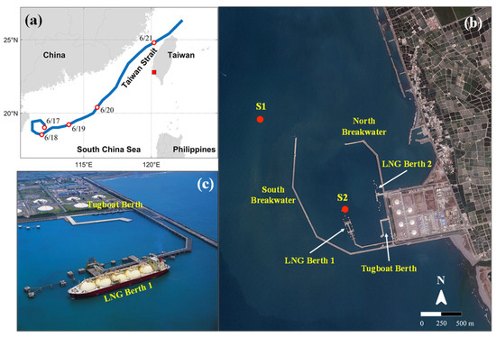
Figure 1.
(a) The geographical location of Youngan Harbor (red square) and the track of Typhoon Talim (2012). (b) A Google image of the harbor, harbor structures, and wave instrument stations S1 and S2 (red circles). (c) An aerial photograph of LNG Berth 1 and the tugboat berth (courtesy of CECI Engineering Consultants, Inc., Taipei, Taiwan).
The harbor is protected from prevailing seasonal waves by a main (southern) breakwater and a secondary (northern) breakwater (Figure 1b). The 2520 m long main breakwater is designed to protect the harbor from predominant southwest waves in the summer. Meanwhile, the 1030 m long secondary breakwater, which extends along the eastern and northern lateral boundaries, shelters the harbor from minor northwest waves in the winter. The 650 m wide harbor entrance is oriented toward the north and directly exposed to the open sea. Additionally, a tugboat dock is located in the corner of the inner basin, enclosing a 320 m long and 90 m wide berthing basin.
The passage of typhoons in the region between the Taiwan Strait and the South China Sea exerts a distinct influence on harbor oscillations, the magnitude of which depends on their distance from the site. Due to the limited protection of the main breakwater against typhoon waves, diffracted swells propagate into the harbor and cause a significant reduction in harbor tranquility. LNG Berth 1 and the tugboat berth are hot spots for this (Figure 1c). The post-typhoon observations made by harbor personnel at LNG Berth 1 indicate that oscillations within the basin can persist for nearly one day after the typhoon warning is lifted before tranquility is fully restored. Furthermore, reported instances of wave overtopping at the tugboat dock present considerable risks to crew safety and the stability of moored barges. These two recurring phenomena, namely the oscillations at LNG Berth 1 and the wave overtopping at the tugboat dock, were the main operational issues observed during typhoon events. Such occurrences reveal critical vulnerabilities of harbor operations under typhoon conditions and underscore the necessity of effective mitigation strategies.
2.2. Field Measurements for Typhoon Waves
According to feedback from harbor personnel, harbor oscillations intensified and persisted for extended periods as typhoons approached the harbor. To investigate this phenomenon, CPC Corporation, which is the harbor authority, conducted short-term wave measurements during selected typhoon events. This study focuses on the dataset collected in June 2012.
Two wave instruments were deployed outside and inside the harbor (Figure 1b). Station S1, located approximately 700 m seaward of the harbor entrance at a water depth of about 16 m, measured offshore wave conditions, while station S2, positioned inside the harbor, recorded wave characteristics near the LNG berth. During the observation period from 17 June to 21 June 2012, Typhoon Talim passed through the study site (Figure 1a). The recorded parameters were significant wave height (HS), peak period (TP), and the corresponding wave direction of TP, as depicted in Figure 2.
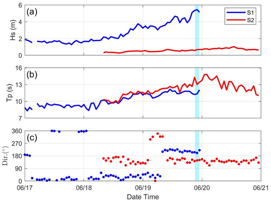
Figure 2.
Wave measurements from 17 to 20 June 2012 at offshore station S1 and in-harbor S2. The plots show (a) significant wave height HS, (b) peak period TP, and (c) wave direction corresponding to TP. The shaded blue interval marks the time of the maximum HS at S1.
Wave information for offshore station S1 was available only until 0:00 on 20 June. The subsequent absence of data was likely due to instrument failure caused by extreme wave conditions as the typhoon transited the study site. This data gap limited the ability to capture the largest wave height during the event. Within the available record at S1, the maximum HS was 5.44 m, with a corresponding TP of 11.34 s and a wave direction from the southwest (220°) at 22:00 on 19 June.
Station S2 began recording wave data at 08:00 on 18 June. S2 measured an HS of 0.68 m with a corresponding TP of 13.02 s when S1 registered its maximum wave height. Measurements at S2 continued until 21 June, during which HS gradually increased, reaching a maximum of 1.03 m with a TP of 12.73 s at 13:00 on 20 June, when data from S1 were unavailable.
A comparison of wave data from the offshore station (S1) and the in-harbor station (S2) during the maximum Hs event at S1 highlights the considerable wave attenuation. The measured HS of 5.44 m at S1 was reduced to 0.68 m at S2, an approximately 87% reduction attributable to the sheltering effect of the breakwaters. The longer TP at S2 reflects the selective attenuation of shorter-period components and the subsequent dominance of relatively longer-period waves within the harbor. Furthermore, the diffracted waves that entered the harbor were trapped, and subsequent multiple reflections resulted in a directional spreading between 120° and 160°, approximately corresponding to the south–southeast sector.
It is important to note that this study was limited by the data provided by the harbor authority, which consisted only of processed bulk wave characteristics. The lack of time series water levels precluded a full spectral analysis to resolve energy contributions across different frequency bands. Consequently, a direct quantification of low-frequency wave energy during the observation period was not possible.
3. Methodology
In this study, two wave-resolving models were employed to simulate typhoon-induced oscillations in the harbor: the Boussinesq-type FUNWAVE-TVD and the non-hydrostatic XBeach (XBeach-NH). Both models have been extensively applied in nearshore hydrodynamic studies and are recognized for their capability to resolve wave transformations and nonlinear interactions. Although the harbor is situated offshore at a depth of approximately 15.0 m, potential reflections from the adjacent coastline and breakwaters could affect long-period oscillations. Appropriate boundary conditions were applied to minimize coastal reflections and ensure that simulated harbor oscillations are primarily driven by offshore incident waves. This configuration allows for a focused comparison of the model performance of nonlinear wave dynamics under predominantly non-breaking conditions. These characteristics make both models suitable for investigating long-period oscillations within the harbor basin. To evaluate model performance, simulated significant wave heights are compared against field observations. This comparative analysis demonstrates the ability of both models to reproduce wave-induced harbor oscillations and supports their application for future harbor tranquility assessments.
3.1. FUNWAVE-TVD Model
The fully nonlinear and dispersive wave model, FUNWAVE-TVD, developed by Shi et al. (2012) [6], is used to numerically simulate nearshore water surface elevations and velocities. The model solves the fully nonlinear Boussinesq equations using a hybrid finite volume-finite difference scheme and incorporates a moving reference level. The governing equations are formulated in a well-balanced conservative form and solved numerically using a total variation diminishing (TVD) scheme, which significantly enhances model stability. The model code is parallelized using domain decomposition with the Message Passing Interface, thus enabling efficient simulations on CPU-based high-performance computing clusters over time scales of several hours.
The governing equations for mass conservation and horizontal momentum equations are given by
where the subscript t denotes time differentiation; ∇ is the horizontal gradient operator; η is the free surface elevation; h is the still water depth; is the velocity at a reference elevation; and is the depth-averaged contribution to the horizontal velocity field. Rs represents the subgrid lateral turbulent mixing, and Rf is the bottom friction parameterized as a quadratic drag law. V1 and V2 represent the Boussinesq dispersion terms, and V3 is the vertical vorticity term. Wave breaking is represented by a shock-capturing approach that locally switches to nonlinear shallow-water equations once a breaking criterion is exceeded or by an eddy-viscosity roller formulation.
3.2. XBeach-NH Model
The XBeach-NH model is based on the incompressible Reynolds-averaged Navier–Stokes equations with a non-hydrostatic pressure term. The governing equations are depth-averaged and consist of the continuity equation:
and the momentum equations:
Here, u, v, and w are the flow velocities in Cartesian coordinates (x, y, and z); represents the turbulent stress tensor; and represents the bottom stress parameterized using a quadratic friction law. The pressure term P is integrated over the vertical direction. A detailed description of equations can be found in a study by Zijlema et al. (2011) [16]. The model treats wave breaking as a sub-grid shock process, in which waves steepen until they are nearly vertical and dissipate energy as a bore. Based on non-hydrostatic principles, the model conserves mass and momentum while including frequency dispersion for accurate breaking-point prediction.
3.3. Model Setup
The model’s bathymetry was derived from a detailed survey conducted in June 2012 by CECI Inc., covering the inner and outer harbor areas. To align the shoreline and contours with the computational grid, the nautical coordinate system was rotated 22.5° clockwise, establishing a local Cartesian coordinate system with the x-axis directed cross-shore and the y-axis alongshore. The computational domain consists of a structured grid of 1200 × 1000 cells with a uniform resolution of 4 m, extending 4.0 km in the x-direction and 4.8 km in the y-direction. The offshore boundary is located approximately 2.6 km seaward of the harbor entrance, where the water depth reaches 20 m. The landward boundary follows the coastline, situated at a depth of approximately 0 m (Figure 3).
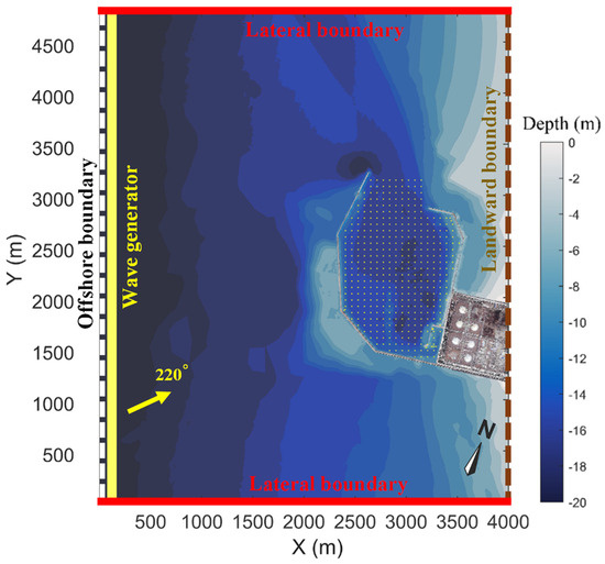
Figure 3.
The computational domain and bathymetry with boundary conditions and a wave generator. Yellow dots mark the locations used for natural mode analysis. The yellow arrow represents the direction of incident waves.
At the offshore boundary, a wavemaker was imposed to generate incident waves characterized by Hs of 5.44 m and peak frequency fP of 0.088 Hz (TP = 11.34 s), observed at station S1. Due to the lack of observed wave spectra, the incident waves were modeled using a JONSWAP spectrum, with a peak enhancement factor of 2.48 following Doong et al. (2015) [17] to represent typhoon conditions in the Taiwan Strait. Unidirectional incident waves were generated from the southwest direction (220°), corresponding to the associated typhoon event. XBeach-NH utilizes an absorbing–generating weakly reflective scheme that enables outgoing long waves to exit with minimal re-reflection. Likewise, FUNWAVE-TVD employs a sponge layer to absorb reflected waves. Although the numerical implementations differ, both boundary treatments aim to suppress spurious reflections and ensure realistic harbor wave dynamics.
In FUNWAVE-TVD, a second-order correction can introduce IG wave components into the offshore waves (Malej et al., 2021) [18]. However, this correction has been found to have a minor influence on the structure and magnitude of resonance modes inside harbors. In addition, this function has not been investigated in XBeach-NH. Accordingly, the input JONSWAP spectrum was restricted to the swell–wind bands (0.05–0.3 Hz), with low-frequency waves below the IG band of 0.05 Hz excluded. This approach is consistent with established research on harbor resonance simulations (Wong, 2016 [14]; Maravelakis et al., 2021 [3]; Thotagamuwage and Pattiaratchi, 2014 [19]).
Lateral boundary conditions were configured differently in the two models. In FUNWAVE-TVD, periodic boundary conditions were imposed, allowing the wave field to wrap continuously around the domain and thereby minimizing artificial reflections. In XBeach-NH, the boundary velocity was prescribed using only the advective terms, following the approach recommended for harbor applications (Wong, 2016) [14]. At the landward boundary, coastal reflections were suppressed to simplify the effect of free IG waves generated by nearshore breaking and refracted by the adjacent coastline. FUNWAVE-TVD applied a sponge layer, whereas XBeach-NH used a weakly reflective absorbing boundary.
To minimize the effect of bottom friction on wave energy inside the harbor, small quadratic friction coefficients for sandy bottoms were prescribed: Cd = 0.001 in FUNWAVE-TVD (Choi et al., 2015) [20] and Cf = 0.001 in XBeach-NH. For the inner harbor boundaries, impermeable structures such as vertical quay walls and breakwaters fronted by armor layers were specified as fully reflective, as long waves experience very limited energy dissipation. Conversely, the pile-supported LNG jetties were modeled as fully transmissive, allowing long waves to propagate through the structures.
3.4. Model Data Analysis
Waves in different frequency bands are known to affect harbor oscillations and ship motions in distinct ways. Short-period swell and wind waves primarily influence ship pitch and roll, while long-period wave motions such as infragravity and very-low-frequency waves are more closely associated with the motions of large ships. In this study, we evaluated three frequency bands: swell and wind-waves (SW) bands, infragravity (IG) bands, and very-low-frequency (VLF) bands. Spectral analysis was applied to model outputs to quantify the power spectral density associated with each frequency component. The significant wave height with a specific frequency band X is defined as (López and Iglesias, 2014) [21]
where Sη(f) denotes the spectral density at frequency f, and and are the lower and upper boundaries of the frequency band X. The overall significant wave height (HS) is calculated over the full frequency range of [0, 0.3 Hz]. The specific band limits for HSW, HIG, and HVLF correspond to frequency ranges [0.05, 0.3 Hz], [0.005, 0.05 Hz], and [0.001, 0.005 Hz], respectively. The significant wave height associated with a natural resonance period T (HT) is obtained by integrating the spectral density over a narrow spectral band centered at f = 1/T.
4. Results and Discussion
4.1. Wave Characteristics at the Measured Location Inside the Harbor
Model validation is typically performed by comparing simulated and observed significant wave heights (HS), as HS serves as a fundamental measure of both wave energy and model accuracy. In common practice, HS is derived from the integration of power spectral densities over the full frequency range, thereby incorporating contributions across all relevant bands (Equation (8)). In the 2012 observational dataset used in this study, the wave instruments recorded 1024 s segments every hour at a 2 Hz sampling resolution. This record length is sufficient to capture the SW and IG bands but is inadequate to resolve VLF motions. Consequently, the measured HS values exclude contributions from the VLF band.
Figure 4 presents a comparison of the simulated HS at station S2 with measurements, along with the decomposed components HSW, HIG, and HVLF from the two models. Both models underestimated HS relative to the measured value of 0.68 m. XBeach-NH showed closer agreement, with a 25% error, compared to 38% for FUNWAVE-TVD. This underestimation of HS by FUNWAVE-TVD in harbor applications is consistent with previous studies (Su and Ma, 2025 [22]; Malej et al., 2021 [18]). Malej et al. (2021) [18] specifically noted model limitations in representing wave diffraction and the scattering of shorter waves, which may have contributed to the underprediction. Similar discrepancies have also been reported for XBeach-NH in harbor environments (Alabart et al., 2014 [23]; Dusseljee et al., 2014 [24]). Collectively, these findings underscore the difficulty both models face in resolving short-wave energy in harbor basins, a factor critical for reliable assessments of harbor tranquility.
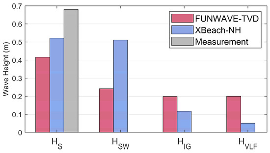
Figure 4.
Comparison of measured and modeled significant wave heights (HS) and decomposed components (HSW, HIG, HVLF) at station S2 from FUNWAVE-TVD and XBeach-NH.
Since the observational dataset does not provide decomposed values for the SW, IG, and VLF bands, the comparison is based solely on the model results. For HSW, XBeach-NH predicted nearly twice the value of FUNWAVE-TVD, thus suggesting stronger short-wave penetration into the harbor. In contrast, FUNWAVE-TVD produced larger HIG and HVLF, implying a more effective nonlinear transfer of energy from shorter to longer periods. The enhanced low-frequency energy of FUNWAVE-TVD is particularly relevant to harbor resonance, as it may contribute to stronger oscillations and longer decay times compared with XBeach-NH.
Figure 5 presents a comparison of the power spectral densities of the two models at station S2. In the SW band, XBeach-NH generally exhibited higher energy densities, although FUNWAVE-TVD produced relatively greater energy at the lower end of this range. At higher SW frequencies, the FUNWAVE-TVD spectrum declined sharply relative to XBeach-NH, primarily due to its inherent limitations in resolving wave diffraction and scattering of high-frequency wave components. In the IG band, FUNWAVE-TVD consistently predicted larger energy densities, particularly at the lower end, suggesting stronger nonlinear wave interactions transferring energy from short to long waves. In the VLF band, FUNWAVE-TVD exceeded XBeach-NH by one to two orders of magnitude. The presence of large VLF waves inside the harbor has been previously documented using FUNWAVE-TVD (Malej et al., 2021 [18]). The existence of large VLF waves was initially attributed to unresolved long-wave reflections from the lateral boundaries, which could contaminate the long-wave field due to accumulation effects during extended simulations. However, in this study, periodic boundary conditions at the lateral boundaries were implemented in FUNWAVE-TVD specifically to minimize reflections. Therefore, the simulated large VLF waves cannot be attributed to the effect of the lateral boundary. This discrepancy between the two models indicates that further field observations are required to clarify the mechanisms governing VLF band dynamics. In addition, the presence of multiple spectral peaks within the IG and VLF bands suggested potential for harbor resonance through coupling with the natural resonance modes of the basin.
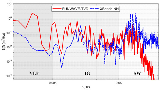
Figure 5.
Modeled spectra at station S2 from FUNWAVE-TVD (solid red line) and XBeach-NH (dashed blue line) at station S2. Gray-shaded regions mark the VLF, IG, and SW frequency bands.
4.2. Spatial Distribution of Wave Heights in SW, IG, and VLF Bands
The spatial distributions of wave heights in the SW, IG, and VLF bands are commonly employed to emphasize the necessity of distinguishing frequency components, since oscillations from different bands affect moored vessels in distinct ways. The distribution of HSW generally reflects the offshore waves penetrating the harbor and their associated diffraction, primarily governing vessel motions in the vertical plane, including heave, pitch, and roll (López and Iglesias, 2014 [21]). In contrast, the distributions of HIG and HVLF reveal the amplification of long waves within harbors, arising from their resonance with the harbor geometry (Wong, 2016 [14]; Malej et al., 2021 [18]; Su and Ma, 2025 [22]). Such long-period oscillations mainly excite horizontal ship motions, particularly sway, surge, and yaw (López and Iglesias, 2014) [21]. Furthermore, harbor resonance has been associated with wave overtopping at harbor structures (Maravelakis et al., 2021) [3]. This phenomenon has been observed by the operational staff at the tugboat dock of Youngan Harbor.
Figure 6 shows the spatial distributions of the simulated HSW, HIG, and HVLF inside the harbor obtained for both models. These results highlight hot spots significantly affected by harbor oscillations. We first examined the FUNWAVE-TVD simulations, with the contour range limited to a maximum of 0.4 m (Figure 6a–c). For HSW, larger values are focused along the interior north breakwater. This pattern arose because diffracted waves penetrating the harbor were reflected from the interior north breakwater and subsequently propagated toward LNG Berth 1 (Goda, 2000) [25]. The tugboat berth, which is the most sheltered area, exhibited the lowest HSW with an average of 0.1 m inside the harbor. For HIG, substantial wave energy was localized along the harbor side of the breakwaters. The largest HIG of approximately 0.8 m occurred in the tugboat berth due to wave trapping and amplification within the confined area. In contrast, relatively low energy appeared in parts of the central basin, including LNG Berth 1. For HVLF, a distinct quasi nodal line developed near the harbor entrance, producing minimal oscillations, whereas an antinode structure occurred in the innermost part of the harbor, leading to considerable energy around the tugboat berth. Therefore, the larger HIG and HVLF around the tugboat berth were consistent with operational staff reports of overtopping at the tugboat dock during typhoon events (Maravelakis et al., 2021) [3].
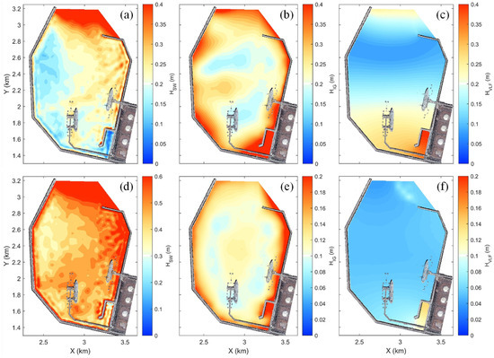
Figure 6.
Spatial distributions of simulated significant wave heights in SW, IG, and VLF bands inside harbor. Panels (a–c) illustrate results from FUNWAVE-TVD, and panels (d–f) illustrate those from XBeach-NH.
The XBeach-NH simulations are presented with contour ranges adjusted to reflect their respective magnitudes in Figure 6d–f. For HSW, the spatial distribution resembled that of FUNWAVE-TVD, with higher values near the north breakwater and lower values near the south breakwater. For HIG, pronounced energy was distributed along the interior sides of breakwaters, forming two quasi nodal lines. LNG Berth 1 was close to one of these nodal lines, which is consistent with the FUNWAVE-TVD result. Additionally, distinct amplification appeared in the tugboat berth, underscoring the tendency of long waves to accumulate within the confined basin. For HVLF, energy levels are generally low throughout the harbor, except for a clear amplification in the tugboat berth.
Both models consistently identified that the largest oscillations occurred in the innermost tugboat berth, where long waves were trapped and amplified within the confined geometry (Su and Ma, 2025) [22]. Overall, the XBeach-NH simulations emphasized the role of short-period SWs in driving harbor oscillations, whereas the FUNWAVE-TVD simulations revealed the dominant influence of long-period IG and VLF waves.
4.3. Identification of Natural Resonance Periods of Harbor
Harbor natural resonance periods are typically characterized by distinct spectral peaks, since low-frequency energy is generally concentrated around resonance modes (Dong et al., 2020 [26]; Thotagamuwage and Pattiaratchi, 2014 [27]; López et al., 2012 [28]). These natural periods are fundamentally determined by harbor geometry and bathymetry (Thotagamuwage and Pattiaratchi, 2014) [19]. However, spectral peaks may be underestimated or even absent if measurements are spatially limited, particularly if instruments are located near the nodal regions of the standing-wave system. Hence, while spectral analysis provides a practical approach for estimating natural periods, reliable identification requires dense measurements covering the entire harbor basin.
To overcome this limitation, a dense grid of 500 points (Figure 3) was uniformly distributed throughout the harbor to simulate water surface elevations, providing a high-resolution spatial coverage. A spectral analysis of the resulting time series was then conducted to identify energy concentrations in the IG and VLF bands. Subsequently, significant peaks were extracted using the MATLAB R2024b (MathWorks, Natick, MA, USA) function findpeaks, which employed a robust adaptive threshold based on the median and median absolute deviation, with constraints on peak height, prominence, and frequency separation. The aggregated peak frequencies were then analyzed using kernel density estimation (KDE) via the MATLAB function ksdensity to obtain a smoothed probability density over frequency (Silverman, 1998) [29]. A higher probability density indicates a greater concentration of spectral peaks around that frequency, thus implying a stronger likelihood of resonance in the corresponding period. Finally, closely spaced peaks in the estimated spectrum were merged to determine robust dominant modes representing the natural resonance periods.
Figure 7 presents the spectral peaks extracted using KDE analysis, which identified the dominant natural resonance periods inside the harbor for the two models. The FUNWAVE-TVD results (Figure 7a) revealed prominent periods at 677 s, 410 s, 186 s, 128 s, 108 s, 85 s, and 64 s. Notably, the model captured VLF oscillations at 677 s and 410 s, indicating high sensitivity to long-period wave dynamics. In contrast, the XBeach-NH results (Figure 7b) showed dominant modes at 254 s, 171 s, 128 s, 89 s, 76 s, and 66 s within the IG band, with the strongest concentration at 89 s. Despite these differences, both models consistently reproduced a robust mode at 128 s and identified resonance modes in comparable frequency ranges. Specifically, FUNWAVE-TVD peaks at 85 s and 64 s correspond closely to XBeach-NH peaks at 89 s and 66 s. Residual discrepancies can be attributed to differences in numerical formulations and their sensitivity to specific long-wave processes.
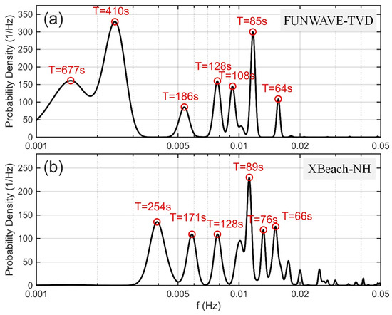
Figure 7.
Dominant resonance periods identified using KDE analysis of spectral probability densities. (a) FUNWAVE-TVD and (b) XBeach-NH model simulations.
Natural resonance periods within the VLF band have been documented in several harbors from long-duration field observations, including 667 s in Marina di Carrara, Italy (Bellotti et al., 2012) [30]; 400 s in Hambantota Port, Sri Lanka (Dong et al., 2020) [26]; 489 s in the harbor of Chania, Greece (Maravelakis et al., 2021) [3]; and 588 s in the Port of Ferrol, Spain (López et al., 2012) [28]. The longer periods simulated by FUNWAVE-TVD, particularly at 677 s and 410 s, are consistent with these reported values. In contrast, XBeach-NH produced only a shorter VLF mode at 254 s. For the comparison of resonance wave heights between the two models, the longest-period VLF mode at 677 s was excluded, since it was not captured by XBeach-NH. This exclusion ensured a consistent and meaningful comparison of the simulated resonance behavior. Table 1 summarizes six peak frequencies within the IG and VLF bands for both models.

Table 1.
Natural resonance periods (in seconds) identified by the two model simulations.
4.4. Spatial Distribution of Natural Resonance Modes
In this section, we investigate the spatial structures of the identified resonance modes to elucidate their distribution within the harbor basin. Analyzing the standing-wave patterns is essential, as it reveals the locations of nodal (minimum oscillation) and antinodal (maximum oscillation) regions. This information is critical for assessing whether specific berths, particularly the LNG and tugboat berths, are affected by harbor resonance. Furthermore, understanding these spatial resonance patterns would provide a crucial basis for mitigation planning and future harbor improvement.
Figure 8 illustrates the spatial distribution of significant wave heights for six resonant modes simulated by FUNWAVE-TVD. For the 410 s mode, the pattern represents a fundamental longitudinal-direction (Y-axis) mode, characterized by a transverse (X-axis) nodal line near the harbor entrance and antinodes at both ends. LNG Berth 1 is located in the transition region of the standing-wave structure, and the tugboat is in the largest antinodal region. For the 186 s mode, the largest antinode appears at the tugboat berth, while much of the harbor basin remains relatively calm. LNG Berth 1 is located in a transitional region of the standing-wave structure, with small wave heights. For the 128 s mode, the longitudinal and transverse nodal lines intersect within the harbor basin, forming four antinodal regions concentrated at the interior breakwater corners. The tugboat berth coincides with an antinodal region, indicating amplified oscillations, whereas LNG Berth 1 lies within a nodal region with minimal oscillations. For the 108 s mode, transverse nodal lines divide the harbor into alternating regions of low and high oscillations. Antinodal regions are concentrated near the breakwater corners, again leading to strong oscillations at the tugboat berth. In contrast, LNG Berth 1 is at a nodal region with minimal oscillations. Finally, the 85 s and 64 s modes exhibit complex resonance characteristics, with alternating nodal and antinodal regions distributed across the basin. For the 85 s mode, amplified oscillations are concentrated at the tugboat berth. In both modes, LNG Berth 1 is generally located near a nodal region with relatively weaker oscillations.
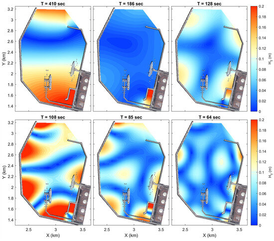
Figure 8.
The spatial distributions of significant wave heights for resonance modes at 410 s, 186 s, 128 s, 108 s, 85 s, and 64 s as simulated by the FUNWAVE-TVD model.
Overall, the analysis reveals that LNG Berth 1 is consistently located within or near the nodal regions of the simulated resonance modes. According to standing-wave theory, these nodal points are characterized by minimal vertical surface oscillation but maximum horizontal current velocity. Therefore, this finding strongly implies that ship motion at LNG Berth 1 at these resonance periods is predominantly induced by horizontal currents associated with nodal standing waves, rather than by direct vertical wave height amplification.
Figure 9 shows the spatial distribution of significant wave heights for six resonant modes simulated by XBeach-NH. The 254 s mode represents a fundamental longitudinal (Y-axis) resonance mode, characterized by a distinct nodal line near the harbor entrance and a wide antinodal region covering the inner harbor basin. LNG Berth 1 is located in the transition region of the standing-wave structure. For the 171 s mode, a node line extends along the longitudinal basin, which is flanked by antinodal regions on either side. The tugboat berth is in an antinodal region, whereas LNG Berth 1 falls within a nodal region. For the 128 s mode, the spatial structure is identical to that simulated by FUNWAVE-TVD, but it exhibits relatively lower wave heights. The 97 s mode is characterized by alternating standing-wave structures, with lower oscillations in the tugboat berth. LNG Berth 1 falls within a nodal region. For the 89 s mode, a pronounced antinode develops at the central basin, surrounded by nodal structures. LNG Berth 1 is located within the region where nodal lines intersect. For the 67 s mode, multiple nodal and antinodal structures appear throughout the basin, producing amplified oscillations along the north breakwater. LNG Berth 1 is again situated in the transition region of a standing-wave structure.
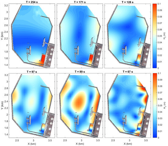
Figure 9.
Spatial distributions of significant wave heights for resonance modes at 254 s, 171 s, 128 s, 97 s, 89 s, and 67 s simulated by XBeach-NH.
In contrast to LNG Berth 1, the harbor authority did not report tranquility problems at LNG Berth 2, which is consistent with the model results. LNG Berth 2 is located near the eastern section of the harbor basin, positioned at the transition zone between an antinode and a node of the standing-wave pattern across all simulated resonance modes (Figure 8 and Figure 9). This region is characterized by mild vertical oscillations and weak horizontal currents, thus resulting in a relatively calm hydrodynamic environment. Consequently, no significant motion or resonance-induced disturbances were observed at LNG Berth 2 during typhoon events.
The comparative study of the spatial distributions of resonance modes obtained from the two model simulations highlights a clear contrast in the impact on key infrastructure. LNG Berth 1 is consistently located in the nodal regions, which are characterized by minimal vertical oscillations but elevated horizontal velocity (López and Iglesias, 2014) [21]. In contrast, the tugboat berth is situated in antinodal regions, where large vertical oscillations occur due to harbor resonance and localized amplification. Therefore, wave overtopping at the tugboat is frequently triggered by typhoon-induced long-period oscillations. To substantiate these modeled mechanisms, current measurements inside the harbor are required to verify the nodal and antinodal structures and confirm the current-driven ship motions inferred at LNG Berth 1.
5. Conclusions
This study compared two wave-resolving models, the Boussinesq-type FUNWAVE-TVD and the non-hydrostatic XBeach-NH, for simulating typhoon-induced oscillations in Youngan Harbor. Both models underestimated the significant wave height across the full frequency range; however, their performance diverged across different frequency bands. XBeach-NH reproduced stronger energy in the swell and wind-wave bands, indicating more pronounced short-wave penetration, whereas FUNWAVE-TVD generated larger energy in the infragravity and very-low-frequency bands, reflecting more effective nonlinear energy transfer to long waves. The resonance analysis clarified the physical mechanisms behind compromised harbor tranquility. LNG Berth 1 was consistently located in nodal regions, where minimal vertical oscillations coincided with elevated horizontal currents that induced ship motions. In contrast, the tugboat berth was situated in antinodal regions, where amplified vertical oscillations explained the recurrent overtopping at the tugboat dock under typhoon conditions. The comparative results showed that no single model was universally superior. Model selection depended on whether short-period swell penetration or long-period infragravity wave resonance was the primary concern, thus suggesting that the complementary use of both models may be beneficial. Future monitoring should include in-harbor current measurements to verify the resonance structure and directly assess ship response. In addition, deploying wave sensors at the tugboat berth and LNG Berth 2 would capture site-specific oscillations, thereby improving model validation. Overall, this study provided a useful framework for future applications of numerical models in harbor tranquility assessment and offered practical insights for harbor management under extreme weather conditions.
Author Contributions
Conceptualization, S.-F.S.; methodology, S.-F.S.; software, I.-A.C.; data curation, P.-W.W.; writing—original draft preparation, S.-F.S.; writing—review and editing, S.-F.S.; visualization, I.-A.C.; supervision, S.-F.S. All authors have read and agreed to the published version of the manuscript.
Funding
This research was primarily supported by the National Science Council of Taiwan (Grant No. 114-2221-E-019-042), with additional support from CECI Engineering Consultants, Inc., Taiwan (Project No. 12947).
Data Availability Statement
The original contributions presented in this study are included in the article. Further inquiries can be directed to the corresponding author.
Conflicts of Interest
Author Pei-Wen Wang was employed by the company CECI Engineering Consultants, Inc. The remaining authors declare that the research was conducted in the absence of any commercial or financial relationships that could be construed as a potential conflict of interest.
References
- Burcharth, H. The lessons learnt from recent breakwater failures: Developments in breakwater design. In Proceedings of the World Federation of Engineering Organizations Technical Congress, Vancouver, BC, Canada, 25–26 May 1987; pp. 1–26. [Google Scholar]
- Rabinovich, A. Chapter 9: Seiches and harbor oscillations. In Handbook of Coastal and Ocean Engineering; Kim, Y.C., Ed.; World Scientific Publishing: Singapore, 2009; pp. 193–236. [Google Scholar]
- Maravelakis, N.; Kalligeris, N.; Lynett, P.J.; Skanavis, V.L.; Synolakis, C.E. Wave overtopping due to harbour resonance. Coast. Eng. 2021, 169, 103973. [Google Scholar] [CrossRef]
- Ardhuin, F.; Rawat, A.; Aucan, J. A numerical model for free infragravity waves: Definition and validation at regional and global scales. Ocean Model. 2014, 77, 20–32. [Google Scholar] [CrossRef]
- Rijnsdorp, D.P.; Reniers, A.J.H.M.; Zijlema, M. Free infragravity waves in the North Sea. J. Geophys. Res. Ocean. 2021, 126, e2021JC017368. [Google Scholar] [CrossRef]
- Shi, F.; Kirby, J.T.; Harris, J.C.; Geiman, J.D.; Grilli, S.T. A high-order adaptive time-stepping TVD solver for Boussinesq modeling of breaking waves and coastal inundation. Ocean Model. 2012, 43–44, 36–51. [Google Scholar] [CrossRef]
- Zijlema, M.; Stelling, G.S. Efficient computation of surf zone waves using the nonlinear shallow water equations with non-hydrostatic pressure. Coast. Eng. 2008, 55, 780–790. [Google Scholar] [CrossRef]
- Guerrini, M.; Bellotti, G.; Fan, Y.; Franco, L. Numerical modelling of long waves amplification at Marina di Carrara harbour. Appl. Ocean Res. 2014, 48, 322–330. [Google Scholar] [CrossRef]
- Bellotti, G.; Franco, L. Measurement of long waves at the harbor of Marina di Carrara, Italy. Ocean Dyn. 2011, 61, 2051–2059. [Google Scholar] [CrossRef]
- Cuomo, G.; Guza, R.T. Infragravity Seiches in a Small Harbor. J. Waterw. Port Coast. Ocean. Eng. 2017, 143, 04017032. [Google Scholar] [CrossRef]
- Kofoed-Hansen, H.; Kerper, D.R.; Sørensen, O.R.; Kirkegaard, J. Simulation of long wave agitation in ports and harbours using a time-domain boussinesq model. In Proceedings of the Fifth International Symposium on Ocean Wave Measurement and Analysis-Waves, Madrid, Spain, 3–7 July 2005; pp. 77–85. [Google Scholar]
- Kwak, M.; Jeong, W.; Kobayashi, N. A case study on harbor oscillations by infragravity waves. Coast. Eng. Proc. 2020, 33. [Google Scholar] [CrossRef]
- Kofoed-Hansen, H.; Sloth, P.; So/rensen Ole, R.; Fuchs, J. Combined Numerical and Physical Modelling of Seiching in Exposed New Marina. In Coastal Engineering 2000; American Society of Civil Engineers (ASCE): Reston, VA, USA, 2012; pp. 3600–3614. [Google Scholar]
- Wong, A. Wave Hydrodynamics in Ports: Numerical Model Assessment of XBeach. Master’s Thesis, Delft University of Technology, Delft, The Netherlands, 2016. [Google Scholar]
- Maroudi, K.A.; Reijmerink, S.P. Advanced modelling of wave penetration in ports. Coast. Eng. Proc. 2020, 36v, waves.18. [Google Scholar] [CrossRef]
- Zijlema, M.; Stelling, G.; Smit, P. Swash: An operational public domain code for simulating wave fields and rapidly varied flows in coastal waters. Coast. Eng. 2011, 58, 992–1012. [Google Scholar] [CrossRef]
- Doong, D.; Tsai, C.; Chen, Y.; Peng, J.; Huang, C. Statistical analysis on the long-term observations of typhoon waves in the Taiwan sea. J. Mar. Sci. Technol. 2015, 23, 8. [Google Scholar] [CrossRef]
- Malej, M.; Shi, F.; Smith, J.M.; Cuomo, G.; Tozer, N. Boussinesq-type modeling of low-frequency wave motions at Marina di Carrara. J. Waterw. Port Coast. Ocean. Eng. 2021, 147, 05021015. [Google Scholar] [CrossRef]
- Thotagamuwage, D.T.; Pattiaratchi, C.B. Influence of offshore topography on infragravity period oscillations in Two Rocks Marina, western Australia. Coast. Eng. 2014, 91, 220–230. [Google Scholar] [CrossRef]
- Choi, J.; Kirby, J.T.; Yoon, S.B. Boussinesq modeling of longshore currents in the SandyDuck experiment under directional random wave conditions. Coast. Eng. 2015, 101, 17–34. [Google Scholar] [CrossRef]
- López, M.; Iglesias, G. Long wave effects on a vessel at berth. Appl. Ocean Res. 2014, 47, 63–72. [Google Scholar] [CrossRef]
- Su, S.-F.; Ma, G. Boussinesq modeling of typhoon-induced infragravity oscillations in Hualien Harbor, eastern Taiwan: Influence of the adjacent coast. Coast. Eng. 2025, 201, 104789. [Google Scholar] [CrossRef]
- Alabart, J.; Sanchez-Arcilla, A.; van Vledder, G.P. Analysis of the performance of swash in harbour domains. In Proceedings of the 3rd IAHR Europe Congress, Porto, Portugal, 14–16 April 2014; Armanini, A., Ed.; IAHR: Madrid, Spain, 2014; pp. 1–10. [Google Scholar]
- Dusseljee, D.W.; Klopman, G.; Van Vledder, G.; Riezebos, H.J. Impact of harbor navigation channels on waves: A numerical modelling guideline. Coast. Eng. Proc. 2014, 1, waves.58. [Google Scholar] [CrossRef]
- Goda, Y. Random seas and design of maritime structures. In Advanced Series on Ocean Engineering; World Scientific: Singapore, 2000; Volume 15, 464p. [Google Scholar]
- Dong, G.; Zheng, Z.; Ma, X.; Huang, X. Characteristics of low-frequency oscillations in the Hambantota port during the southwest monsoon. Ocean Eng. 2020, 208, 107408. [Google Scholar] [CrossRef]
- Thotagamuwage, D.T.; Pattiaratchi, C.B. Observations of infragravity period oscillations in a small marina. Ocean Eng. 2014, 88, 435–445. [Google Scholar] [CrossRef]
- López, M.; Iglesias, G.; Kobayashi, N. Long period oscillations and tidal level in the Port of Ferrol. Appl. Ocean Res. 2012, 38, 126–134. [Google Scholar] [CrossRef]
- Silverman, B.W. Density Estimation for Statistics and Data Analysis, 1st ed.; Routledge: London, UK, 1998. [Google Scholar] [CrossRef]
- Bellotti, G.; Briganti, R.; Beltrami, G.M.; Franco, L. Modal analysis of semi-enclosed basins. Coast. Eng. 2012, 64, 16–25. [Google Scholar] [CrossRef]
Disclaimer/Publisher’s Note: The statements, opinions and data contained in all publications are solely those of the individual author(s) and contributor(s) and not of MDPI and/or the editor(s). MDPI and/or the editor(s) disclaim responsibility for any injury to people or property resulting from any ideas, methods, instructions or products referred to in the content. |
© 2025 by the authors. Licensee MDPI, Basel, Switzerland. This article is an open access article distributed under the terms and conditions of the Creative Commons Attribution (CC BY) license (https://creativecommons.org/licenses/by/4.0/).