Research on a Real-Time Prediction Method of Hull Girder Loads Based on Different Recurrent Neural Network Models

Abstract

Real-time prediction of hull girder loads is of great significance for the safety of ship structures. Some scholars have used neural network technology to investigate hull girder load real-time prediction methods based on motion monitoring data. With the development of deep learning technology, a variety of recurrent neural networks have been proposed; however, there is still a lack of systematic comparative analysis on the prediction performance of different networks. In addition, the real motion monitoring data inevitably contains noise, and the effect of data noise has not been fully considered in previous studies. In this paper, four different recurrent neural network models are comparatively investigated, and the effect of different levels of noise on the prediction accuracy of various load components is systematically analyzed. It is found that the GRU network is suitable for predicting the torsional moment and horizontal bending moment, and the LSTM network is suitable for predicting the vertical bending moment. Although filtering has been applied to the original noise data, the prediction accuracy still decreased as the noise level increased. The prediction accuracy of the vertical bending moment and horizontal bending moment is higher than that of the torsional moment.

1. Introduction

The hull girder loads are an important factor affecting the overall structural safety of ships, which is a key focus in the design and use of ship structures [1,2]. Real-time prediction of hull girder load data will be of great help to the captain’s navigation decision-making, especially in high-sea conditions when the hull girder loads are large and there is a high risk of failure in the ship’s structure.

The Hull Response Monitoring System (HRMS) is a system that measures and displays ship structure stress, ship structure strain, and ship motion data. Many scholars have established a real-time prediction method for hull girder loads based on real-time strain monitoring data by utilizing the mechanical relationship between hull girder loads and structural strain [3,4,5,6,7,8]. Strain sensors on the hull structure may experience data drift and other issues during long-term use, which can lead to incorrect reporting of the hull girder loads. Compared with the strain gauge data, the ship motions are more accessible to obtain and more stable. For ships without HRMS installed, the hull girder loads can be indirectly predicted through motion monitoring data. For ships that have already been installed with HRMS, the hull girder loads obtained by using motion data and strain data can be compared to ensure the accuracy of hull girder load measurements further.

Xu [9] developed a methodology for estimating wave-induced vertical bending moments from heave and pitch measurements based on artificial neural networks. The artificial neural networks were trained by using the auto- and cross-correlation functions of the bending moment and the ship motions. The prediction model has been validated through a comparison of experimental data. Moreira and Guedes Soares [10] presented a neural network model for the estimation of hull bending moment and shear force of ships in waves. The ship motion and hull girder loads were simulated by using a time domain strip method [11], and then a reasonable network model was established to estimate the instantaneous bending moment and shear force by analyzing the effect of different numbers of neurons. Xu et al. [12] also utilized an improved BP neural network to investigate the prediction method of sectional shear force and bending moment based on ship motion data. Previous research tends to focus more on utilizing networks to train the correlation between motion and hull girder loads. However, due to the memory effect of waves, ship motion and hull girder loads exhibit strong temporal correlations.

With the advancement of networks, recurrent neural networks (RNNs) with long-term memory effects are increasingly being utilized in the fields of ship and ocean engineering. Liu et al. [13] presented a model for the reconstruction and prediction of global whipping responses on a large cruise ship based on Long Short-Term Memory (LSTM) neural networks. Su et al. [14] introduced a real-time algorithm for predicting ship vertical acceleration using the LSTM and GRU models. Based on the database originating from a commercial professional simulator, Li et al. [15] predicted short-term ship roll motion by leveraging the encoder–decoder structure of Bidirectional Long Short-Term Memory Networks (Bi-LSTM) with teacher forcing. Fan et al. [16] combined the different empirical mode decomposition methods with LSTM networks to effectively predict short-term offshore structure motions. Liu et al. [17] proposed an input vector space optimization for the LSTM deep learning model in real-time prediction of ship motions. Xie et al. [18] introduced a mooring line tension model based on the GRU network, which accurately predicts mooring line tension using wave elevation components or float motion responses.

Many scholars use recurrent neural networks to solve time-series problems with temporal correlations in the ship and ocean engineering field. However, the performance of different RNNs in real-time prediction of the hull girder loads still lacks systematic research. In addition, real-time monitoring data of ship motion, as input data for the real-time prediction model of the hull girder load, inevitably contains certain noise components. However, there is a lack of detailed analysis of the impact of noise on motion input data in previous studies.

In this paper, the real-time prediction method of hull girder loads is investigated by using several different recurrent neural network models. The performance of different recurrent neural networks is systematically compared and analyzed. The method of controlling variables is used for hyperparameter optimization. Taking into account the characteristic that the ship motion data contains noise, a new prediction procedure combining filtering techniques to reduce the influence of noise is established. In addition, the effect of different levels of noise on the prediction accuracy of hull girder loads is systematically analyzed.

2. Hull Girder Loads Prediction Model

2.1. Basic Concepts of RNN

Simple recurrent networks can theoretically establish dependencies between states with long-time intervals. The gradient explosion or gradient vanishing problem restricts the learning of only short-term dependencies. The Long Short-Term Memory Network (LSTM) is a variant of recurrent neural networks that can effectively solve the problems of gradient explosion or vanishing encountered in simple RNNs. The LSTM model calculates the gradient through the backpropagation through time (BPTT) algorithm and then adjusts the model weight and bias parameters until convergence. The sensitivity of the model to time is reflected in the three gating units (input gate, forgetting gate, and output gate) that control the information flow. Through these three gating units, information can be selectively remembered and forgotten [19].

The Gated Recurrent Unit (GRU) network represents a simpler form of the recurrent neural network compared to the LSTM network. It incorporates a gating mechanism to regulate the update of information. Unlike LSTM, GRU omits an additional memory unit and employs an update gate to determine the amount of historical state information to retain in the current state, as well as how much new information from the candidate set should be considered for inclusion [20].

Increasing the depth of recurrent neural networks enhances model performance, commonly achieved by stacking multiple recurrent networks, forming a Stacked Recurrent Neural Network (SRNN). A Bidirectional Recurrent Neural Network (BI-RNN) comprises two layers of recurrent neural networks with identical inputs, differing only in the direction of information flow. In conjunction with the LSTM neural network and the GRU neural network, the bidirectional recurrent neural network may encompass a bidirectional long short-term memory (BI-LSTM) neural network [15] and a bidirectional gated recurrent unit (BI-GRU) neural network [21].

2.2. Input and Output Data

In this study, the RNN models are developed to predict the hull girder loads by the known ship motion responses. A container ship is chosen as the research object, and the numerical simulation of the ship is conducted in the time domain. The specific parameters are shown in the following Section 3.1, taking the ship’s heave motion, pitch motion, and roll motion as input, and the vertical bending moment, horizontal bending moment, and torsional moment at the midship section as output. After giving the complete input and output time histories of each operating sea state in the data of RNN models, the data are divided into the training and validating sets, which are respectively used for training the RNN models and validating the accuracy of the predicting results from the trained RNN models. In addition, the validating sets should be independent of the training sets; that is, validating sets do not participate in the training process of the neural network model.

The motion data of the ship obtained by the hull response monitoring systems (HRMS) are usually accompanied by a significant amount of noise. Numerical motion data obtained from simulations are artificially augmented with numerical noise, forming testing sets with motion input data that includes noise. The testing sets are designed with inputs of data containing various levels of noise to test the accuracy of the predicted results.

2.3. Data Pre-Processing

The normalized data can enhance the convergence speed of the network model and improve the prediction performance. Input and output data often differ significantly in their numerical values and dimensions. Normalization helps to eliminate these differences and achieve consistency in the data, facilitating more effective training of the model.

$$x\prime =\frac{x-x_{\min }}{x_{\max }-x_{\min }}$$

(1)

where $x^{\prime }$ is the normalized input or output data, $x$ is the original data, and $x_{\max }$ and $x_{\min }$ are the maximum and minimum value in the sequence, respectively. To ensure a meaningful comparison with the actual hull girder load sequence, it is necessary to apply an inverse normalization to the predicted results.

2.4. Evaluation Criterion

Evaluation criteria are crucial parameters for evaluating the prediction performance of the model. Root Mean Square Error (RMSE), Mean Absolute Percentage Error (MAPE), and Pearson’s correlation coefficient ($\rho$) are selected.

$RMSE$ represents the standard deviation of the residuals between the predicted and actual values, providing a measure of error discretization. It is defined as

$$RMSE=\sqrt{\raisebox{1ex}{$1$}\!\left/ \!\raisebox{-1ex}{$n$}\right.{\displaystyle \sum _{i=1}^n{(y_i^{origin}-y_i^{pred})}^2}}$$

(2)

where $y_i^{origin}$ is the actual value, $y_i^{pred}$ is the predicted value, $n$ represents the quantity of data, and the range of the $RMSE$ value is $\left[0,+\infty \right]$, which is equal to 0 if the predicted value exactly matches the true value; the larger the error, the larger the value.

$MAPE$ is a percentage representation of the MAE, which is the average of the absolute value of the error:

$$MAPE=\frac{100\%}{n}{\displaystyle \sum _{i=1}^n\left|\frac{y_i^{origin}-y_i^{pred}}{y_i^{origin}}\right|}$$

(3)

where $y_i^{origin}$ is the actual value, $y_i^{pred}$ is the predicted value, and $n$ represents the quantity of data. The range of $MAPE$ is $\left[0,+\infty \right]$ and a $MAPE$ of 0% indicates a perfect model; the closer the value is to 0, the better the model’s predictive accuracy.

Pearson’s correlation coefficient quantifies the linear relationship between two random variables. The concept of correlation coefficient is introduced:

$$\rho =Corr(X,Y)=\frac{Cov(X,Y)}{\sigma X\cdot \sigma Y}$$

(4)

Here, $\sigma X, \sigma Y$ represent the standard deviations of variables $X,Y$, respectively. $Cov(X,Y)$ is the covariance of $X,Y$. The closer the correlation coefficient ($\rho$) is to 1, the stronger the correlation in the model and the more accurate the model prediction.

3. Physics-Based Numerical Simulation

3.1. Simulation Model

A large container ship is selected as the object of this paper. Table 1 shows the main parameters of the container ship. Motion simulation in irregular waves is conducted using the commercial software Wasim to generate databases of ship motion responses and hull girder loads. Wasim is a three-dimensional hydrodynamic analysis software based on potential flow theory in the time domain; it can predict ship motion responses in waves with the Rankine panel method and considers many nonlinear factors. The fluid dynamic pressure field can be generated based on Bernoulli’s equation. The d’Alembert principle is used to solve the sectional-induced loads of the ship in waves.

Table 1. Container ship’s principal dimensions.

Length	Width	Depth	Structural Draught	Speed	Block Coefficient
278 m	32.2 m	23.3 m	13 m	23 kn	0.7

Figure 1 illustrates the wet surface mesh. The Pierson–Moskowitz (PM) spectrum is chosen as a wave spectrum to describe irregular waves. Irregular waves are represented using 200 sub-waves. Eight percent of the critical damping is applied to roll motion. The control of gravity is assigned as (124.63 m, 0, 10.22 m). A non-linear solver is employed for the 3 h time domain simulation.

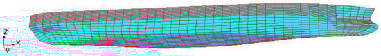
Figure 1. Wet surface mesh.

3.2. Simulation Load Case

The databases of ship motion responses and hull girder loads under different short-term sea conditions are established to train the network models. Parameters related to short-term sea conditions include significant wave height H_s, average zero-crossing period T_z, wave direction $\beta$, and ship speed $v$. When the sea condition parameters encountered during the ship’s voyage are the same as those in the training database, the data have strong relevance, which may lead to higher forecast accuracy.

Considering that the actual sea conditions experienced by the ship may not be consistent with the sea conditions in the training set, the load case in Table 2 is designed to verify the predictive ability of the neural network model. The sea state parameters encountered by the ship are assumed to be H_s = 11 m, T_z = 11 s, $\beta$ = 135°, and $v$ = 7.5 kn, as indicated in Table 2 for the testing database. Sixteen sets of short-term sea conditions for numerical simulation are assumed as the training and validating databases. In subsequent practical applications, it is only necessary to further increase the number of samples in the training set to obtain a neural network model with a wider applicability.

Table 2. Loadcase parameters of B_MULTI.

Load Case	Databases	Significant Wave $\mathbf{Height}{\mathit{H}}_{\mathit{s}}$ (m)	Zero-Crossing $\mathbf{Periods}{\mathit{T}}_{\mathit{z}}$ (s)	Wave Direction $\mathit{\beta }$ (°)	Velocity $\mathit{v}$ (kn)
B_MULTI	Training and validating	10.5	10.5	120	5
		10.5	10.5	120	10
		10.5	10.5	150	5
		10.5	10.5	150	10
		10.5	11.5	120	5
		10.5	11.5	120	10
		10.5	11.5	150	5
		10.5	11.5	150	10
		11.5	10.5	120	5
		11.5	10.5	120	10
		11.5	10.5	150	5
		11.5	10.5	150	10
		11.5	11.5	120	5
		11.5	11.5	120	10
		11.5	11.5	150	5
		11.5	11.5	150	10
	Testing	11	11	135	7.5

4. Results and Discussion

4.1. Determination of Network Structures of Different RNN Models

The training process of the neural network is to find the suitable fitting function in the hypothesis space on a certain number of training data. The control variable method is the common method to find the optimal model by adjusting the single variable and maintaining other variables unchanged [16,22,23]. In this section, the influence of window length, optimizers, layer number, and neuron number on the accuracy of hull girder loads prediction models will be studied in turn.

4.1.1. Determination of Window Length

The variation in window length is one of the key factors affecting the prediction accuracy of the model. When the window length is set to ‘a’, its physical meaning is that the motion data from the previous ‘a’ time steps are used as inputs, and the ship hull girder loads at the ‘a’th time step are used as the output. By sliding the window, multiple databases of motion inputs and ship hull girder load outputs are obtained.

For the torsional moment (TM) prediction model, to investigate the impact of different window lengths on network prediction performance, window lengths of 50, 100, 150, and 200 are analyzed. A single-layer neural network with 32 neurons and the ‘adam’ optimizer is chosen, and four networks—LSTM, GRU, BI-LSTM, and BI-GRU—are separately trained.

The GRU network model exhibits the highest prediction accuracy, followed by the BI-GRU network model, whereas the LSTM and BI-LSTM network models demonstrate lower prediction accuracy and larger errors, as shown in Figure 2 and Figure 3 For the GRU network, a window length of 150 yields $\rho$ = 0.772, and RMSE = 0.051, significantly outperforming the window length of 50 and slightly outperforming the window lengths of 100 and 200. The window lengths of 150, 100, and 150 are the optimal window lengths for the LSTM, BI-LSTM, and BI-GRU networks, respectively.

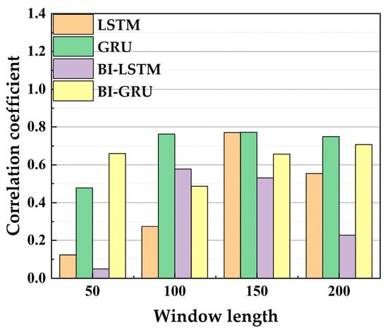
Figure 2. Correlation coefficient (TM model).

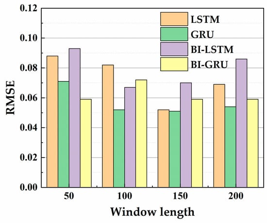
Figure 3. RMSE (TM model).

For the vertical bending moment (VBM) prediction model, a single-layer neural network with 32 neurons using the ‘adam’ optimizer was chosen. The evaluation index value for a window length of 150 is slightly higher than that for the other three lengths, indicating that the accuracy of the four neural network models is not significantly affected by changes in window length, as shown in Figure 4 and Figure 5. For a window length of 150, the precision ($\rho$) of all four networks exceeds 0.9, and the RMSE is less than 0.037. Specifically, the LSTM network model achieves the highest precision of $\rho$ = 0.935 and RMSE = 0.032 among all networks. The window lengths of 150, 100, and 150 are the optimal window lengths for the GRU, BI-LSTM, and BI-GRU networks, respectively.

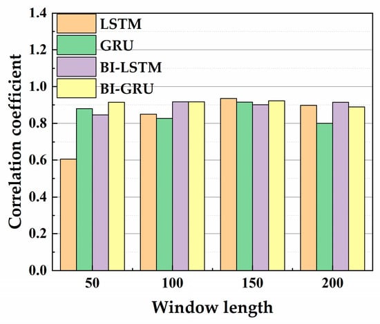
Figure 4. Correlation coefficient (VBM model).

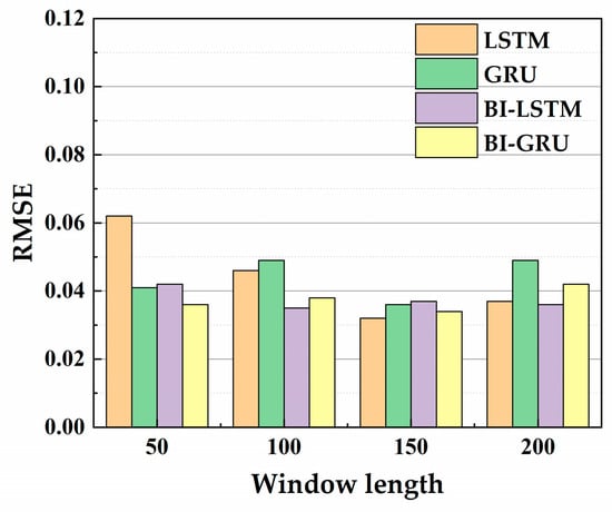
Figure 5. RMSE (VBM model).

For the horizontal bending moment (HBM) prediction model, a single-layer neural network with 64 neurons using the ‘adam’ optimizer is employed. The GRU network model exhibits the highest prediction accuracy, followed by the BI-GRU network model, while the prediction accuracy of the LSTM and BI-LSTM network models is slightly lower, as shown in Figure 6 and Figure 7. Among GRU networks, at a window length of 150, $\rho$ = 0.837 and RMSE = 0.057, demonstrating notably superior performance compared to a window length of 100, and marginally better performance compared to window lengths of 50 and 200. The window lengths of 200, 200, and 200 are the optimal window lengths for the LSTM, BI-LSTM, and BI-GRU networks, respectively.

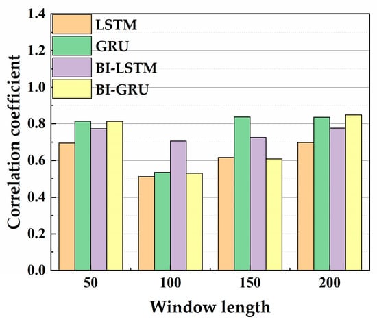
Figure 6. Correlation coefficient (HBM model).

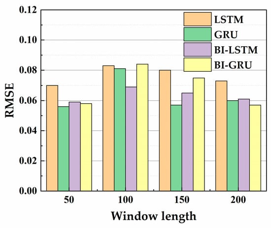
Figure 7. RMSE (HBM model).

4.1.2. Determination of Optimizers

The variation in optimizers is another one of the key factors affecting the prediction accuracy of the model. The role of the optimizer in the backpropagation process of deep learning is to guide the parameters of the loss function to update in the correct direction with an appropriate magnitude, allowing the loss function to gradually approach or achieve its minimum value.

For the TM prediction model, to investigate the impact of different optimizers on network prediction performance, optimizers of SGD, adam, RMSprop, and Nadam are analyzed. A single-layer neural network with 32 neurons and a window length of 150 is chosen, and four networks—LSTM, GRU, BI-LSTM, and BI-GRU—are separately trained.

Figure 8 and Figure 9 illustrate that the adam and Nadam optimizers achieve relatively high prediction accuracy across all four neural network models, surpassing significantly the accuracy obtained with SGD and RMSprop optimizers. Among the four models, the traditional optimizer SGD exhibits the lowest prediction accuracy. Among the four network models, the GRU network demonstrates the highest prediction accuracy, followed by the LSTM network. Regarding the GRU network, the adam optimizer yields significantly better prediction accuracy compared to RMSprop and slightly outperforms the Nadam optimizer, as shown in Figure 10. The adam optimizer exhibits results closest to the actual values; hence it is selected for constructing the GRU network. The optimizer of adam is also the optimal optimizer for LSTM and BI-GRU. Nadam is the optimal optimizer for the BI-LSTM network.

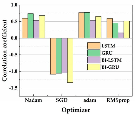
Figure 8. Correlation coefficient (TM model).

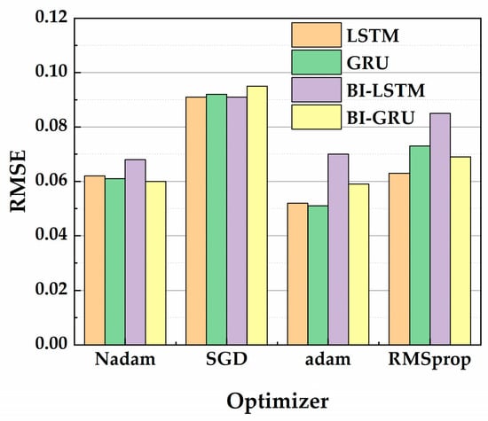
Figure 9. RMSE (TM model).

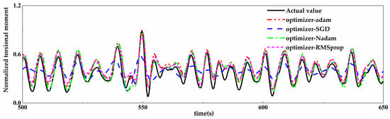
Figure 10. Prediction results under different optimizers (GRU network).

For the VBM prediction model, a single-layer neural network with 32 neurons and a window length of 150 is used. As shown in Figure 11 and Figure 12, it is evident that the adam, Nadam, and RMSprop optimizers have relatively higher prediction accuracy than the SGD optimizers. The LSTM network model demonstrates the highest prediction accuracy among the four network models, followed by the BI-GRU network model. In LSTM networks, the prediction accuracy achieved with the adam optimizer is comparable to that obtained with RMSprop and Nadam. Figure 13 illustrates the prediction results obtained with different optimizers in the LSTM network. The adam optimizer yields predictions closest to the true values; thus, it is selected for constructing the LSTM network. The optimizer of adam is also the optimal optimizer for GRU and BI-GRU. RMSprop is the optimal optimizer for the BI-LSTM network.

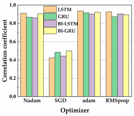
Figure 11. Correlation coefficient (VBM model).

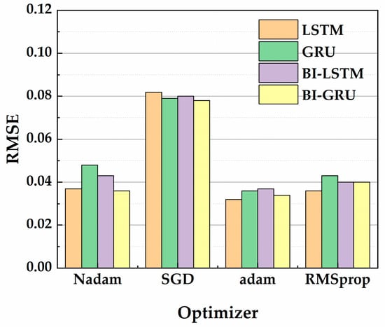
Figure 12. RMSE (VBM model).

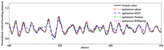
Figure 13. Prediction results under different optimizers (LSTM network).

For the HBM prediction model, a single-layer neural network with 64 neurons and a window length of 150 is used. As shown in Figure 14 and Figure 15, the adam optimizer consistently yields relatively high prediction accuracy across all four neural network models, slightly outperforming the Nadam optimizer. Conversely, the RMSprop optimizer exhibits relatively low prediction accuracy, while the SGD optimizer, the most traditional choice, performs the worst among the four models. Among the four network models, the GRU network model achieves the highest prediction accuracy, followed by the BI-LSTM network model. In GRU networks, the adam optimizer yields slightly higher prediction accuracy compared to the Nadam and RMSprop optimizers. Figure 16 illustrates the prediction results obtained with different optimizers in the GRU network. The adam optimizer yields predictions closest to the true values; thus, it is selected for constructing the GRU network. The optimizer of adam is also the optimal optimizer for LSTM and BI-LSTM. Nadam is the optimal optimizer for the BI-GRU network.

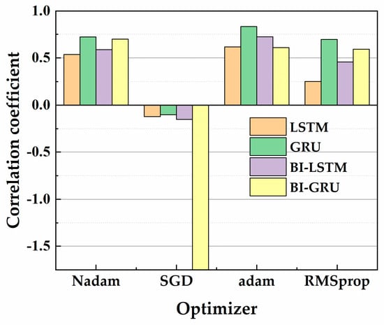
Figure 14. Correlation coefficient (HBM model).

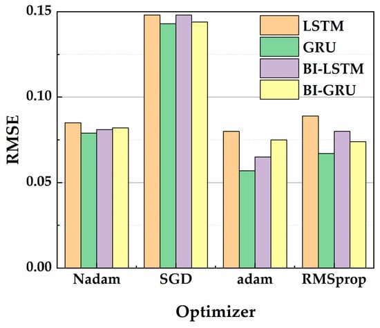
Figure 15. RMSE (HBM model).

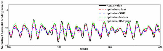
Figure 16. Prediction results under different optimizers (GRU network).

4.1.3. Coupling Determination of the Layer and Neuron Number

The number of neurons and the depth of the neural network are the key factors affecting the prediction accuracy of the model. Considering the coupled impact of the number of network layers and the number of neurons on the network’s prediction accuracy, the most suitable network structure is identified.

For the TM prediction model, to investigate the impact of different numbers of network layers and neurons on network prediction performance, nine types of network structure were analyzed. A window length of 150 and the ‘adam’ optimizer are chosen. Table 3 illustrates the number of network layers and neurons.

Table 3. Number of network layers and number of neurons (TM model).

Item	1-1	1-2	1-3	2-1	2-2	2-3	3-1	3-2	3-3
Network Layers	1	1	1	2	2	2	3	3	3
Number of neurons	16	32	64	16-8	32-16	32-32	16-32-16	32-32-32	64-32-16

Figure 17 and Figure 18 illustrate that for a single layer (layer = 1), the BI-LSTM network achieves the highest prediction accuracy with $\rho$ = 0.846 and RMSE = 0.043; for two layers (layer = 2), the GRU network exhibits the highest prediction accuracy with $\rho$ = 0.767 and RMSE = 0.054; and for three layers (layer = 3), the GRU network attains the highest prediction accuracy with $\rho$ = 0.853 and RMSE = 0.042. For a single layer (layer = 1), the prediction accuracy of the network rises with an increasing number of neurons; while for three layers (layer = 3) with 32 neurons each, the network achieves the highest prediction accuracy. Figure 19 illustrates the prediction results of the GRU network with different numbers of hidden layers.

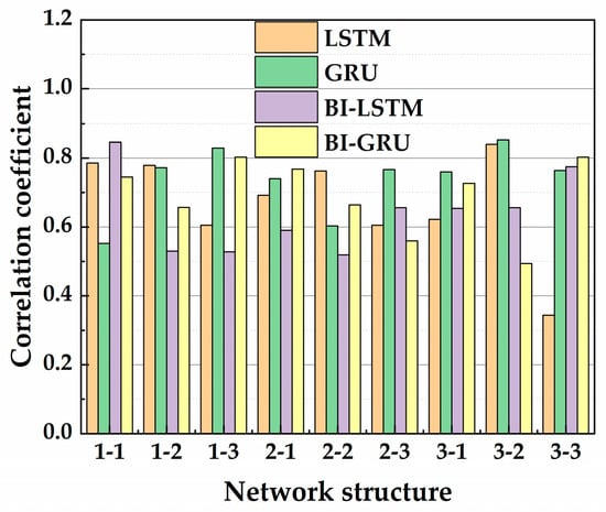
Figure 17. Correlation coefficient (TM model).

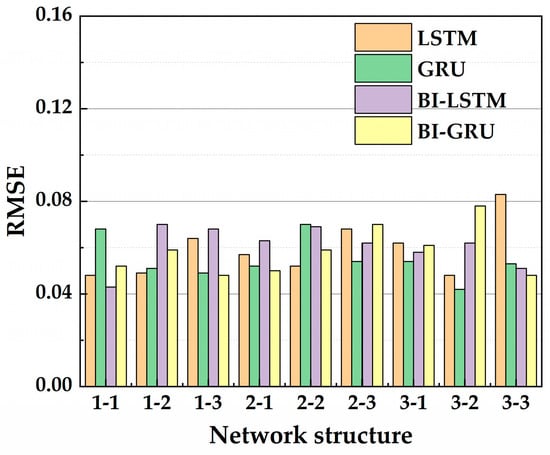
Figure 18. RMSE (TM model).

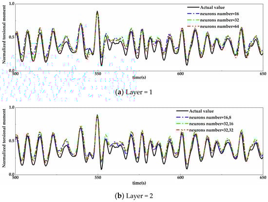
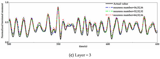
Figure 19. Prediction results under different network structures (GRU network).

In the case of a three-layer GRU network, changing the number of neurons per layer to 64, 32, and 16 results in lower prediction accuracy compared to when the number of neurons remains consistent at 32 for all layers. This suggests that excessive neurons may lead to overfitting. Moreover, having varying numbers of neurons for the same number of layers does not necessarily improve performance; hence, thorough parameter discussion is crucial to determine the optimal settings. The three-layer networks with 32 neurons each and the single-layer networks with 16 neurons and 64 neurons are the optimal network structures for LSTM, BI-LSTM, and BI-GRU networks, respectively.

For the VBM prediction model, four different numbers of hidden layers and various numbers of neurons are chosen to analyze the influence of coupling parameters. The window length is set to 150, and the ‘adam’ optimizer is employed. Table 4 illustrates the number of network layers and neurons.

Table 4. Number of network layers and number of neurons (VBM model).

Item	1-1	1-2	1-3	2-1	2-2	3-1	4-1
Network Layers	1	1	1	2	2	3	4
Number of neurons	8	16	32	16-8	32-16	16-32-16	16-32-32-16

Figure 20 and Figure 21 illustrate that when the number of layers is set to 1, the prediction accuracy of all networks increases as the number of neurons increases. Figure 22 illustrates the prediction results obtained with different numbers of neurons in a single-layer LSTM network. When the number of neurons is set to 32, all four networks achieve a prediction accuracy of over 0.9. The highest prediction accuracy is achieved with 32 neurons in the LSTM network. When the number of layers is 2, 3, and 4, despite the gradual increase in the number of layers, the number of neurons also increases. However, the prediction accuracy of all four networks remains around 0.8–0.9. The networks show insensitivity to changes in the number of layers and neurons, but increasing the number of layers and neurons prolongs the training time. The single-layer LSTM network model demonstrates relatively high prediction accuracy and training efficiency. The two-layer networks with 16-8 neurons, the three-layer networks with 16-32-16 neurons, and the one-layer network with 32 neurons are the optimal network structures for GRU, BI-LSTM, and BI-GRU networks, respectively.

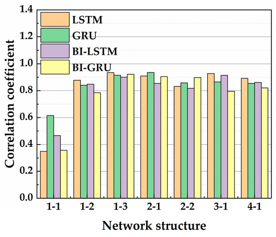
Figure 20. Correlation coefficient (VBM model).

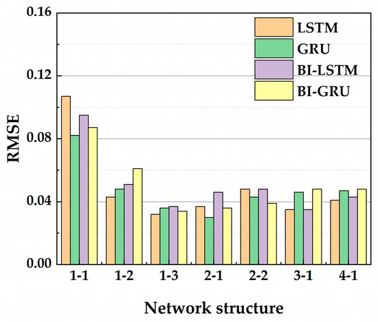
Figure 21. RMSE (VBM model).

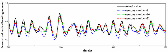
Figure 22. Prediction results under different network structures (LSTM network, layer = 1).

For the HBM prediction model, nine types of network structure were analyzed. A window length of 150 and the ‘adam’ optimizer is chosen. Table 5 illustrates the number of network layers and neurons.

Table 5. Number of network layers and number of neurons (HBM model).

Item	1-1	1-2	1-3	2-1	2-2	2-3	3-1	3-2	3-3
Network Layers	1	1	1	2	2	2	3	3	3
Number of neurons	16	32	64	16-8	32-16	32-32	16-32-16	32-32-32	64-32-16

Figure 23 and Figure 24 illustrate that when the number of layers is set to 1, the GRU network achieves the highest prediction accuracy at $\rho$ = 0.837 and RMSE = 0.057. With two layers, the GRU network attains the highest prediction accuracy at $\rho$ = 0.883 and RMSE = 0.046. Similarly, with three layers, the GRU network exhibits the highest prediction accuracy at $\rho$ = 0.901 and RMSE = 0.045. Figure 25 illustrates the prediction results of the GRU network with varying numbers of hidden layers. The network achieves the highest prediction accuracy when it has three layers and each layer has 32 neurons. The three-layer networks with 32 neurons each are also the optimal network structures for LSTM, BI-LSTM, and BI-GRU networks, respectively.

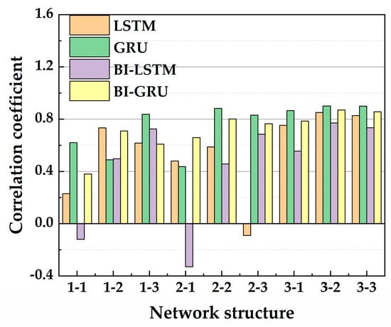
Figure 23. Correlation coefficient (HBM model).

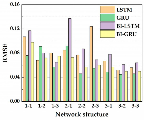
Figure 24. RMSE (HBM model).

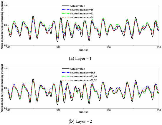
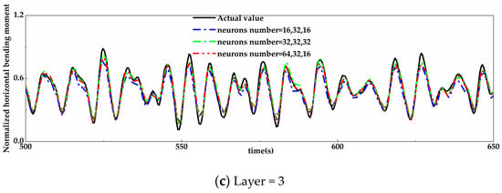
Figure 25. Prediction results under different network structures (GRU network).

4.2. Prediction of Different Network Models Using Motion Data with The Same Noise

4.2.1. Numerical Noise

The ship motion data obtained by the hull response monitoring systems (HRMS) is usually accompanied by a large amount of noise. In order to make the simulation data of the testing database similar to the actual ship monitoring data, different levels of numerical noise are artificially added to the simulated data of the testing database. The ship motion data with noise is used as input to verify the prediction accuracy and noise resistance of the ship hull girder load prediction model established in this paper. The motion response to noise can be represented by the following equation:

$$Y=Y^{true}+l\cdot std(Y^{true})\cdot randn$$

(5)

Here, $Y^{true}$ represents the simulation ship motion response, $std(Y^{true})$ represents the standard deviation of the calculated response, $l$ denotes the noise level, and $randn$ refers to a set of random numbers with a mean of 0 and a variance of 1.

Three levels of noise ($l=5\%$, $l=10\%$, and $l=15\%$) were added to the original numerical simulation ship motion data. Figure 26 illustrates a comparison between the time histories of heave motion data and the corresponding data with three levels of noise. It is evident that the deviation from the true value increases with higher noise levels.

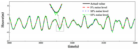
Figure 26. Heave motion data with three levels of noise.

4.2.2. Filtering Technique

When directly using the motion data with added noise for ship hull girder load prediction, the presence of noise often tends to further amplify its impact on the prediction results, leading to greater high-frequency oscillation outputs, as shown in Figure 27. Typically, existing HRMS usually filter real-time monitoring data to mitigate noise effects. The purpose of filtering processing is to eliminate the unrealistic high-frequency oscillation noise. Fast Fourier Transform (FFT) filtering is a noise reduction method widely adopted for experimental data [24,25] and actual monitoring data [26,27]. The basic principle of FFT filtering is to operate on the frequency composition of the signal in the frequency domain to alter its frequency characteristics. By analyzing the frequency, it is possible to filter out the inauthentic high-frequency oscillations that represent noise, thereby extracting pure ship motion data.

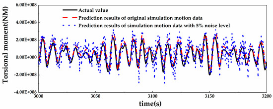
Figure 27. Direct prediction results of 5% noise level.

Spectral analysis is conducted on both the original time-series data and the time-series data with varying levels of noise, as illustrated in Figure 28. It can be observed that selecting a cutoff frequency of 0.2 Hz is appropriate, as it can filter out high-frequency noise at various noise levels. As the noise level increases, the deviation between the filtered data and the original data also increases. To more clearly express the deviation between the filtered data and the original data, the overall standard deviation $\sigma$ is used to represent the degree of deviation:

$$\sigma =\sqrt{{\displaystyle \sum _{i=1}^n{(x_i^{original}-x_i^{filtered})}^2}/n}\times 100\%$$

(6)

where $x_i^{filtered}$ represents the filtered data at $t=i$, $x_i^{original}$ represents the original data at $t=i$, and $n$ represents the total number of moments. For noise level $l=5\%$, $\sigma =4.01\%$. For noise level $l=10\%$, $\sigma =7.89\%$. For noise level $l=15\%$, $\sigma =12.75\%$.

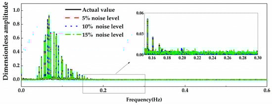
Figure 28. Spectral analysis.

4.2.3. Prediction Results

Through the parameter analysis in Section 4.1, the optimal parameters for the four network models suitable for predicting the hull girder loads have been identified, as shown in Table 6. For the original simulation data without added noise, the prediction results of some models are quite similar. For example, taking the TM prediction as an example, the results from the three-layer GRU network and the single-layer BI-LSTM are both relatively high, with the prediction results not exceeding 1%.

Table 6. Optimal parameter combinations for the four network models.

model	LSTM			GRU
	window length	optimizer	network structure	window length	optimizer	network structure
TM	150	adam	3, 32-32-32	150	adam	3, 32-32-32
VBM	150	adam	1, 32	150	adam	2, 16-8
HBM	200	adam	3, 32-32-32	150	adam	3, 32-32-32
model	BI-LSTM			BI-GRU
	window length	optimizer	network structure	window length	optimizer	network structure
TM	100	Nadam	1, 16	150	adam	1, 64
VBM	100	RMSprop	3, 16-32-16	150	adam	1, 32
HBM	200	adam	3, 32-32-32	200	Nadam	3, 32-32-32

In order to further compare the prediction performance of different models on input data with noise, the motion input data with the same noise level are used to validate. The motion data with a noise level $l=10\%$ are selected. According to Section 4.2.2, the cut-off frequency of 0.2 Hz is chosen to filter the data with noise.

Table 7 illustrates the evaluation index values for the four network models. For the TM prediction model, the GRU network exhibits higher prediction accuracy and noise resistance. For the VBM prediction model, the four network models exhibit similar and relatively high prediction accuracies, the $\rho$ of all four networks remains around 0.87. For the HBM prediction model, compared to the other networks, the GRU network has a slight advantage. Therefore, Table 8 presents the optimal model types and model parameters for predicting torsional moment (TM), vertical bending moment (VBM), and horizontal bending moment (HBM).

Table 7. Evaluation index values for the four network models.

model	LSTM			GRU
	$\rho$	RMSE	MAPE	$\rho$	RMSE	MAPE
TM	0.608	0.089	7.50%	0.660	0.085	7.40%
VBM	0.873	0.050	3.90%	0.875	0.052	4.00%
HBM	0.841	0.052	4.00%	0.886	0.050	3.80%
model	BI-LSTM			BI-GRU
	$\rho$	RMSE	MAPE	$\rho$	RMSE	MAPE
TM	0.583	0.090	8.30%	0.612	0.092	8.50%
VBM	0.876	0.051	4.00%	0.873	0.050	4.00%
HBM	0.838	0.057	4.20%	0.845	0.054	4.30%

Table 8. Optimal network models for hull girder loads prediction.

Model	Type	Window Length	Optimizer	Network Structure
TM	GRU	150	adam	3, 32-32-32
VBM	LSTM	150	adam	1, 32
HBM	GRU	150	adam	3, 32-32-32

4.3. Prediction of the Same Network Models Using Motion Data with Different Noise

In order to test the prediction accuracy of the ship hull girder load models for input data with different noise levels, the original motion response data without noise and with noise level $l=5\%$, $l=10\%$, $l=15\%$ are designed. The evaluation index values are listed in Table 9.

Table 9. Evaluation index values of load case B_MULTI.

Motion Data	TM			VBM			HBM
	$\mathit{\rho }$	RMSE	MAPE	$\mathit{\rho }$	RMSE	MAPE	$\mathit{\rho }$	RMSE	MAPE
Origin	0.743	0.073	6.20%	0.913	0.042	3.30%	0.945	0.036	2.40%
5% noise	0.729	0.075	6.40%	0.887	0.048	3.60%	0.904	0.046	3.60%
10% noise	0.660	0.085	7.40%	0.873	0.050	3.90%	0.886	0.050	3.80%
15% noise	0.697	0.082	7.10%	0.838	0.062	5.60%	0.850	0.056	4.50%

When the original motion input data is without noise, the test procedure of this paper is similar to the study of Moreira and Guedes Soares [10]. The databases of wave-induced vertical bending moment and shear force prediction model are established based on theoretical methods. When the significant wave height is 3 m, the correlation coefficients of VBM of ADEE ship and Grand America Ro-Ro are 0.8945 and 0.607, respectively. The prediction accuracy of the VBM model of the present study is 0.913. It is obvious that the LSTM model has better prediction performance than the ANN model. As the level of noise increases, the prediction accuracy gradually decreases. For motion input data with a noise of 15%, $\rho$ = 0.838 and MAPE = 5.60%. Figure 29 presents the prediction results under different levels of noise. When the noise level is at 15%, the prediction values closely align with the actual values.

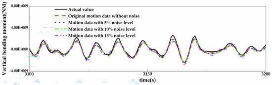
Figure 29. Prediction results under different noise levels (VBM prediction model).

Another advantage of the present paper is its ability to predict horizontal bending moments (HBM) and torsional moments (TM). The prediction accuracy of the HBM model is the highest. For motion input data without added noise, $\rho$ = 0.945 and MAPE = 2.40%. As the level of noise increases, the prediction accuracy gradually decreases. For motion input data with a noise of 15%, $\rho$ = 0.85 and MAPE = 4.50%. Figure 30 presents the prediction results under different levels of noise. When the noise level is at 15%, the prediction values closely align with the actual values.

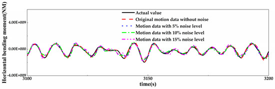
Figure 30. Prediction results under different noise levels (HBM prediction model).

The prediction accuracy of the TM model is the lowest. For motion input data without added noise, $\rho$ = 0.743 and MAPE = 6.20%. As the level of noise increases, the prediction accuracy gradually decreases. For motion input data with a noise of 15%, $\rho$ = 0.697 and MAPE = 7.10%. Figure 31 presents the prediction results under different levels of noise. While the prediction values at a 5% noise level closely align with the actual values, those at 10% and 15% noise levels significantly deviate from actual values.

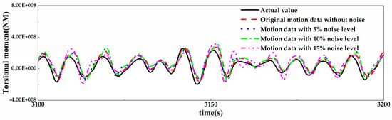
Figure 31. Prediction results under different noise levels (TM prediction model).

In summary, although all noisy data have been subjected to filtering, an increase in the noise level will still lead to poorer prediction results. Filtering techniques cannot filter noisy data to be the same as the original data. Instead, the lower the noise level, the lower the degree of dispersion in the results after filtering, as discussed in Section 4.2.2. When the input data are the original motion response data without noise, the prediction accuracy of the VBM and HBM models is about 22% higher than the TM model. When the input data are the original motion response data with a 15% noise level, the prediction accuracy of VBM and HBM models remains 20% higher than the TM model.

5. Conclusions

This paper proposes a real-time prediction method of hull girder loads considering the noise in motion monitoring data. Four improved recurrent neural networks are used to establish the hull girder load prediction models. The commercial software Wasim is utilized to acquire databases of ship motion response and hull girder loads in waves. Numerical noise is introduced to the ship’s motion response data to emulate real ship motion monitoring data. The following conclusions are drawn:

(1)

The method of controlling variables is used for hyperparameter optimization. Without considering data noise, the optimal network structures of the hull girder load prediction model are respectively obtained based on four improved recurrent neural networks (LSTM, GRU, BI-LSTM, and BI-GRU networks). It found that the most suitable type of recurrent neural network for different load components (TM, VBM, and HBM) is different. The three-layer GRU network with 32 neurons each is the optimal network structure for predicting TM and HBM, and the one-layer LSTM with 32 neurons is the optimal network structure for predicting VBM.

(2)

The real-time prediction model of hull girder load takes ship motion monitoring data as input in practical applications, and motion monitoring data inevitably contain certain noise. It is found that directly using motion monitoring data as input for the real-time prediction of hull girder loads will result in significant prediction errors. Therefore, a numerical filtering method is proposed to preprocess the motion monitoring data. The results indicate that the filtering preprocessing method can significantly improve the prediction accuracy of the model. Using the prediction model that considers the effect of motion data noise, the performance of four improved recurrent neural networks is further analyzed. It is also found that the three-layer GRU network with 32 neurons each is the optimal network structure for predicting TM and HBM, and the one-layer LSTM with 32 neurons is the optimal network structure for predicting VBM.

(3)

The prediction accuracy of the optimal network models for input data with different levels of noise is discussed. It found that although filtering was applied to the original noise data, the prediction accuracy of the model still decreased as the noise level increased. For both the original input data and noisy input data, the prediction accuracy of VBM and HBM is consistently more than 20% higher than that of TM.

Using neural networks to predict hull girder load is a new research direction for the ship structure problem, and it will be of great significance for ship hull intellectualization. There are still some shortcomings in the present study, which need to be improved in the follow-up research.

Due to the lack of actual monitoring data, the model established in this paper lacks validation with actual monitoring data. If actual ship monitoring data can be obtained in the future, the prediction models can be used for further verification.

This paper takes a container ship as an example to propose a prediction method. Other types of ships can also refer to the method proposed in this paper to establish a ship hull girder load prediction model suitable for themselves. The model established in this paper can be further verified for other ship types and other working conditions in future research.

References

- Mohammed, E.A.; Benson, S.D.; Hirdaris, S.E.; Dow, R.S. Design safety margin of a 10,000 TEU container ship through ultimate hull girder load combination analysis. Mar. Struct. 2016, 46, 78–101. [Google Scholar] [CrossRef]
- Amlashi, H.K.K.; Moan, T. A proposal of reliability-based design formats for ultimate hull girder strength checks for bulk carriers under combined global and local loadings. J. Mar. Sci. Technol. 2011, 16, 51–67. [Google Scholar] [CrossRef]
- Almallah, I.; Lavroff, J.; Holloway, D.S.; Shabani, B.; Davis, M.R. Global load determination of high-speed wave-piercing catamarans using finite element method and linear least squares applied to sea trial strain measurements. J. Mar. Sci. Technol. 2020, 25, 901–913. [Google Scholar] [CrossRef]
- Torkildsen, H.E.; Grøvlen, Å.; Skaugen, A.; Wang, G.; Jensen, A.E.; Pran, K.; Sagvolden, G. Development and Applications of Full-Scale Ship Hull Health Monitoring Systems for the Royal Norwegian Navy. In Recent Developments in Non-Intrusive Measurement Technology for Military Application on Model- and Full-Scale Vehicles; RTO: Neuilly-sur-Seine, France, 2005. [Google Scholar]
- Fanelli, P.; Mercuri, A.; Trupiano, S.; Vivio, F.; Falcucci, G.; Jannelli, E. Live reconstruction of global loads on a powerboat using local strain FBG measurements. Procedia Struct. Integr. 2019, 24, 949–960. [Google Scholar] [CrossRef]
- Zhang, M.; Sun, L.H.; Xie, Y.G. A monitoring method of hull structural bending and torsional moment. Ocean. Eng. 2024, 291, 116344. [Google Scholar] [CrossRef]
- Tayyar, G.T. Overall hull girder nonlinear strength monitoring based on inclinometer sensor data. Int. J. Nav. Archit. Ocean. Eng. 2020, 12, 902–909. [Google Scholar] [CrossRef]
- Kefal, A.; Oterkus, E. Displacement and stress monitoring of a chemical tanker based on inverse finite element method. Ocean. Eng. 2016, 112, 33–46. [Google Scholar] [CrossRef]
- Xu, J.Z. Estimation of wave-induced ship hull bending moment from ship motion measurements. Mar. Struct. 2000, 14, 593–610. [Google Scholar] [CrossRef]
- Moreira, L.; Guedes Soares, C. Neural network model for estimation of hull bending moment and shear force of ships in waves. Ocean. Eng. 2020, 206, 107347. [Google Scholar] [CrossRef]
- Fonseca, N.; Soares, C.G. Experimental investigation of the nonlinear effects on the statistics of vertical motions and loads of a containership in irregular waves. J. Ship Res. 2004, 48, 148–167. [Google Scholar] [CrossRef]
- Xu, W.; Li, H.; Ying, Y.; Zhang, M. Prediction of Total Force and Moment of Ship Based on Improved BP Neural Network. In Proceedings of the 8th International Technical Conference on Frontiers of Hydraulic and Civil Engineering Technology, HCET 2023, Wuhan, China, 25–27 September 2023; pp. 1420–1435. [Google Scholar]
- Liu, R.X.; Li, H.; Zou, J.; Ong, M.C. Reconstruction and prediction of global whipping responses on a large cruise ship based on LSTM neural networks. Ocean. Eng. 2023, 285, 115393. [Google Scholar] [CrossRef]
- Su, Y.M.; Lin, J.F.; Zhao, D.G.; Guo, C.Y.; Wang, C.; Guo, H. Real-Time Prediction of Large-Scale Ship Model Vertical Acceleration Based on Recurrent Neural Network. J. Mar. Sci. Eng. 2020, 8, 777. [Google Scholar] [CrossRef]
- Li, S.Y.; Wang, T.T.; Li, G.Y.; Skulstad, R.; Zhang, H.X. Short-term ship roll motion prediction using the encoder-decoder Bi-LSTM with teacher forcing. Ocean. Eng. 2024, 295, 116917. [Google Scholar] [CrossRef]
- Fan, G.J.; Yu, P.Y.; Wang, Q.; Dong, Y.K. Short-term motion prediction of a semi-submersible by combining LSTM neural network and different signal decomposition methods. Ocean. Eng. 2023, 267, 113266. [Google Scholar] [CrossRef]
- Liu, Y.C.; Duan, W.Y.; Huang, L.M.; Duan, S.L.; Ma, X.W. The input vector space optimization for LSTM deep learning model in real-time prediction of ship motions. Ocean. Eng. 2020, 213, 107681. [Google Scholar] [CrossRef]
- Xie, Y.J.; Tang, H.S.; Low, Y.M. Deep gated recurrent unit networks for time-domain long-term fatigue analysis of mooring lines considering wave directionality. Ocean. Eng. 2023, 284, 115244. [Google Scholar] [CrossRef]
- Zhang, T.; Zheng, X.Q.; Liu, M.X. Multiscale attention-based LSTM for ship motion prediction. Ocean. Eng. 2021, 230, 109066. [Google Scholar] [CrossRef]
- Liu, H.D.; Liu, Y.; Li, B.; Qi, Z.G. Ship Abnormal Behavior Detection Method Based on Optimized GRU Network. J. Mar. Sci. Eng. 2022, 10, 249. [Google Scholar] [CrossRef]
- Li, H.H.; Xing, W.B.; Jiao, H.; Yang, Z.L.; Li, Y. Deep bi-directional information-empowered ship trajectory prediction for maritime autonomous surface ships. Transp. Res. Part E-Logist. Transp. Rev. 2024, 181, 103367. [Google Scholar] [CrossRef]
- Wang, Z.M.; Qiao, D.S.; Yan, J.; Tang, G.Q.; Li, B.B.; Ning, D.Z. A new approach to predict dynamic mooring tension using LSTM neural network based on responses of floating structure. Ocean. Eng. 2022, 249, 110905. [Google Scholar] [CrossRef]
- Qiao, D.S.; Li, P.; Ma, G.; Qi, X.L.; Yan, J.; Ning, D.Z.; Li, B.B. Realtime prediction of dynamic mooring lines responses with LSTM neural network model. Ocean. Eng. 2021, 219, 108368. [Google Scholar] [CrossRef]
- Xie, H.; Ren, H.; Deng, B.; Tang, H. Experimental drop test investigation into slamming loads on a truncated 3D bow flare model. Ocean. Eng. 2018, 169, 567–585. [Google Scholar] [CrossRef]
- Wang, Q.; Yu, P.; Fan, G.; Li, G. Experimental drop test investigation into cross deck slamming loads on a trimaran. Ocean. Eng. 2021, 240, 109999. [Google Scholar] [CrossRef]
- Lay-Ekuakille, A.; Vendramin, G.; Trotta, A. Spectral analysis of leak detection in a zigzag pipeline: A filter diagonalization method-based algorithm application. Measurement 2009, 42, 358–367. [Google Scholar] [CrossRef]
- Thirumala, K.; Umarikar, A.C.; Jain, T. An improved adaptive filtering approach for power quality analysis of time-varying waveforms. Measurement 2019, 131, 677–685. [Google Scholar] [CrossRef]
Disclaimer/Publisher’s Note: The statements, opinions and data contained in all publications are solely those of the individual author(s) and contributor(s) and not of MDPI and/or the editor(s). MDPI and/or the editor(s) disclaim responsibility for any injury to people or property resulting from any ideas, methods, instructions or products referred to in the content. |
© 2024 by the authors. Licensee MDPI, Basel, Switzerland. This article is an open access article distributed under the terms and conditions of the Creative Commons Attribution (CC BY) license (https://creativecommons.org/licenses/by/4.0/).