


A Low-Cost Communication-Based Autonomous Underwater Vehicle Positioning System


 , , and
Abstract
1. Introduction
2. Existing Methodologies
2.1. Multiple-Transponder Systems
- Long baseline (LBL) and GPS intelligent buoy (GIB): One of the first UWA localization techniques developed in the middle of the 1970s by [11]. The long baseline (LBL) procedure consists of a set of UWA transponders precisely disposed of on the seabed around the mission area. Each transponder has a known precise position and is synchronized with the others. Therefore, in addition to beacon deployment, the calibration of their relative position and timing becomes a key step. The AUV position is then estimated through triangulation with respect to its range to all transponders. Ranges are computed with TOF or time difference of arrival (TDOA) techniques. At least three transponders are recommended to have good accuracy. The GPS intelligent buoy (GIB) method is similar to LBL. The difference is that transponders are installed on surface buoys and not on the seafloor. This reduces calibration costs.
- Short baseline (SBL): Beacons are deployed at opposite sides of a surface vessel (or platform). TDOA triangulation is then used to determine the AUV position. The baseline length is designed in relationship with the vessel size. The main limitation of short baseline (SBL) is its localization accuracy.
2.2. Single-Transponder Systems
3. Materials and Methods
3.1. Problem Formulation
3.2. Drone Scheduling
3.3. AUV Model
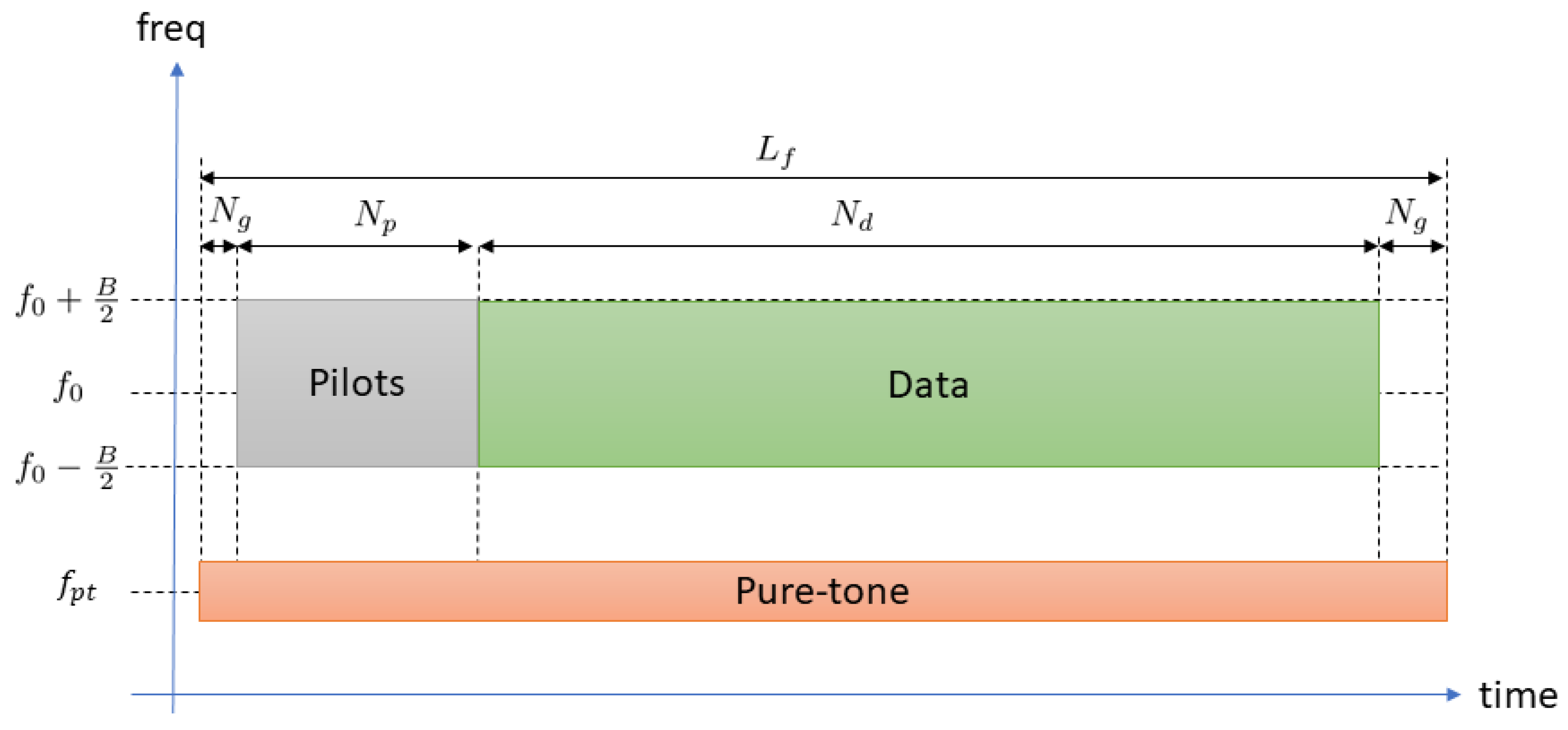
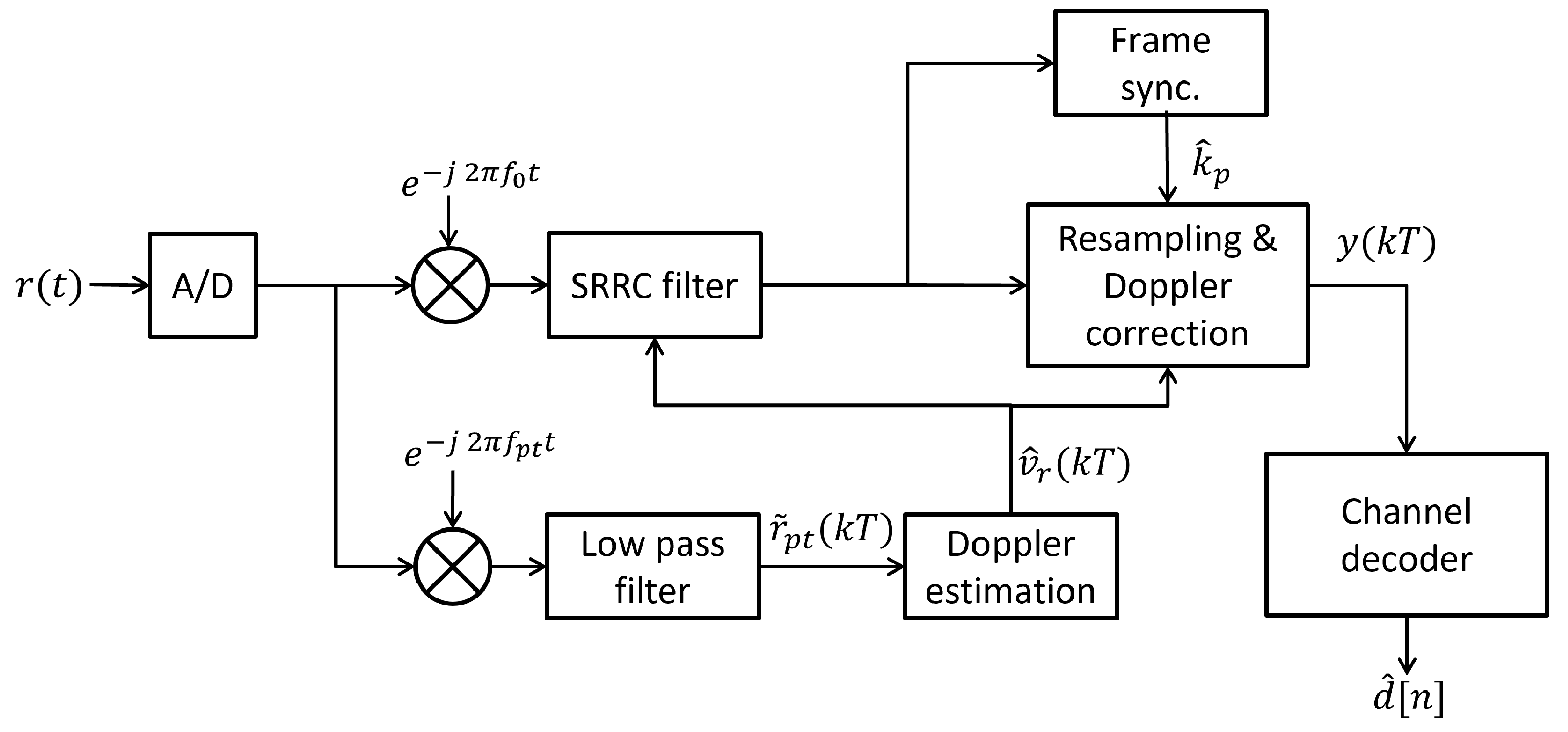
3.4. Underwater Acoustic Communication System
3.5. Measurements
3.5.1. Distance Estimation
3.5.2. Speed Estimation
3.5.3. Proprioceptive Sensors
3.5.4. Equations
3.6. Estimator Filter
| Algorithm 1: Extended Kalman Filter |
| Data: , , , |
| Result: , |
| 1 |
| 2 |
| 3 |
| 4 |
| 5 |
| 6 |
| 7 |
| 8 |
4. Results
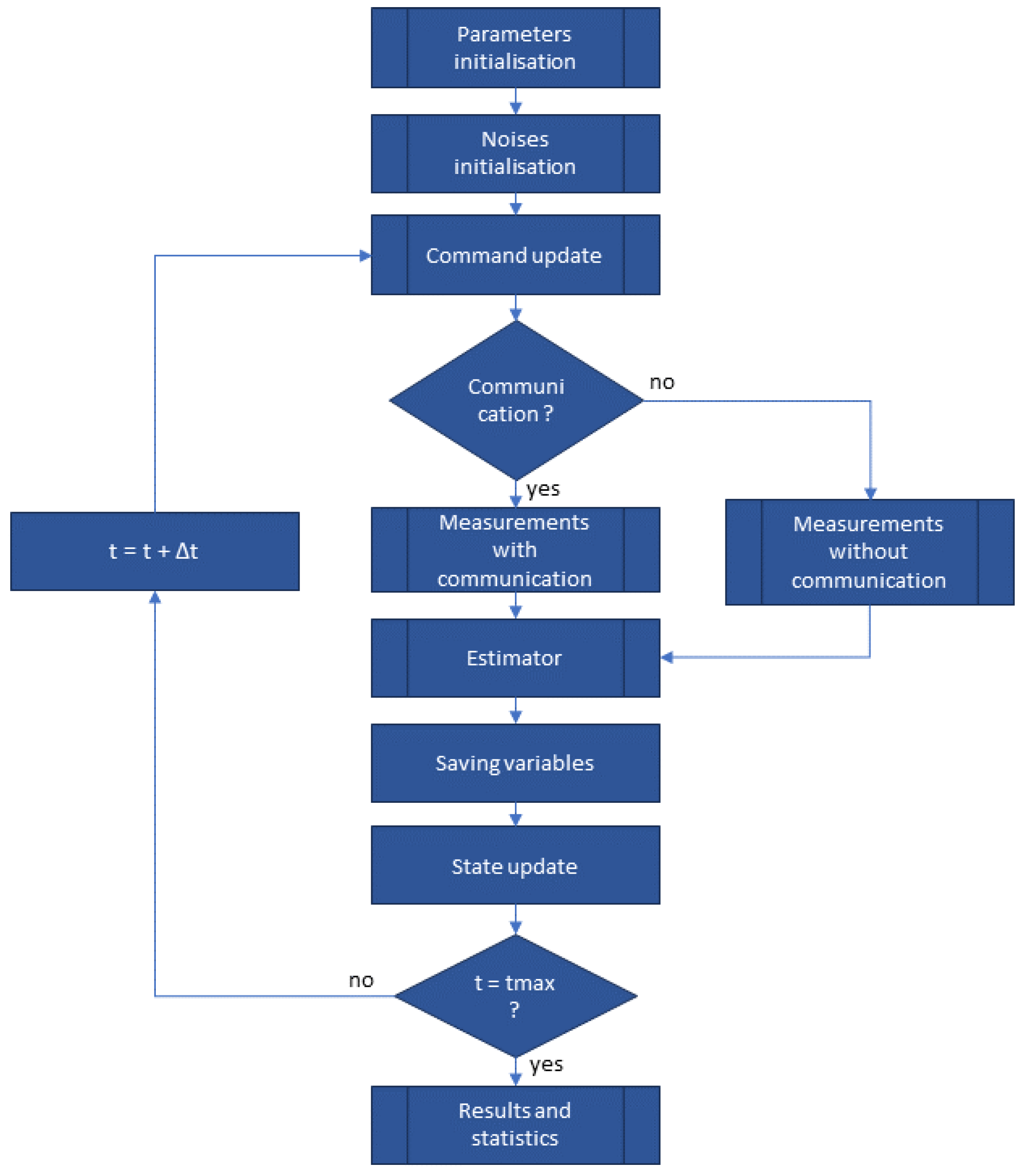
4.1. Simulation
4.1.1. Parameters
- Mean positioning error;
- Variance of the positioning error;
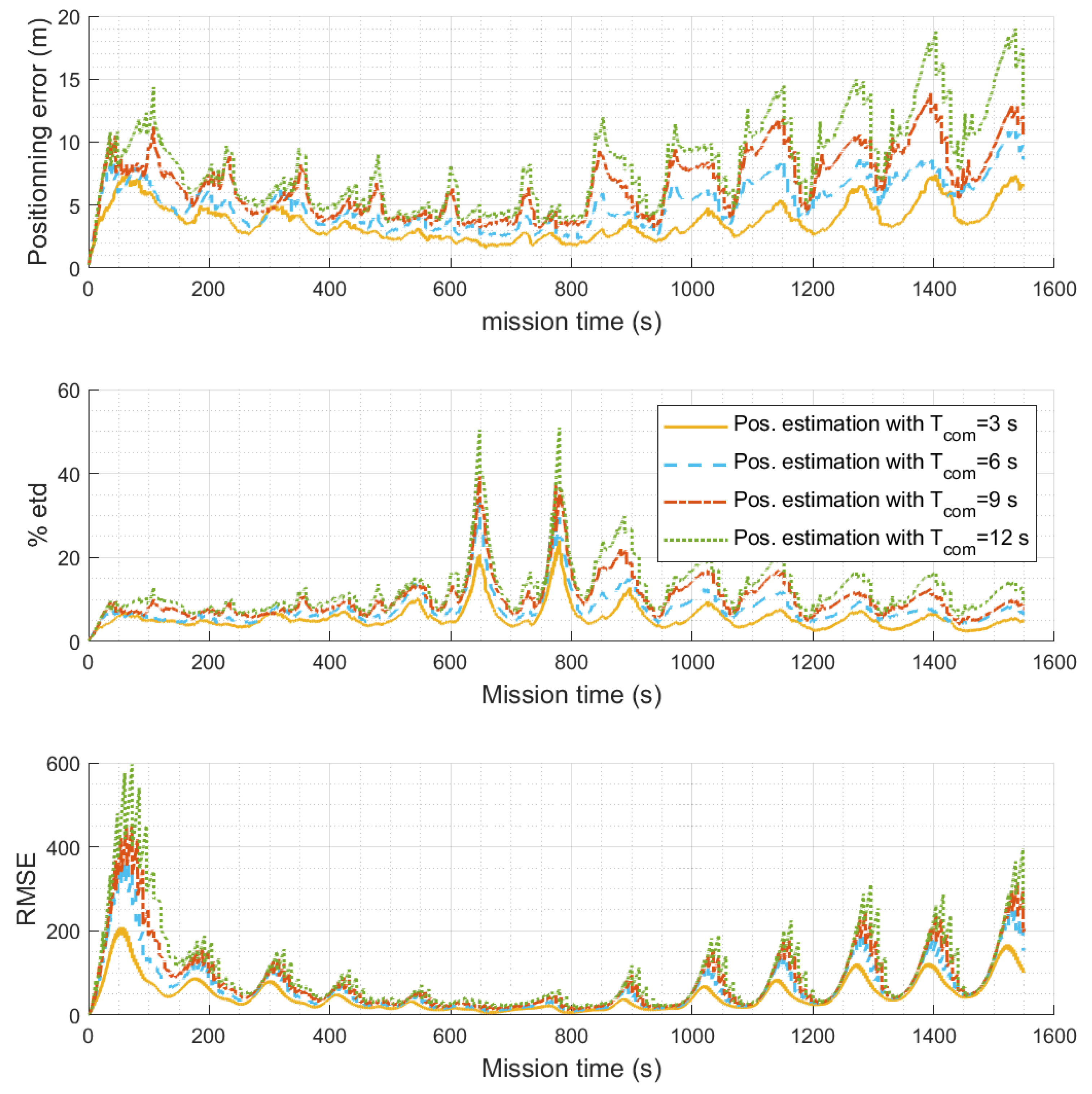
- Root mean square error and positioning error curves;
- Noises for each measurement;
- Bearing angle estimation errors.
4.1.2. Simulation Results
4.2. Experiments
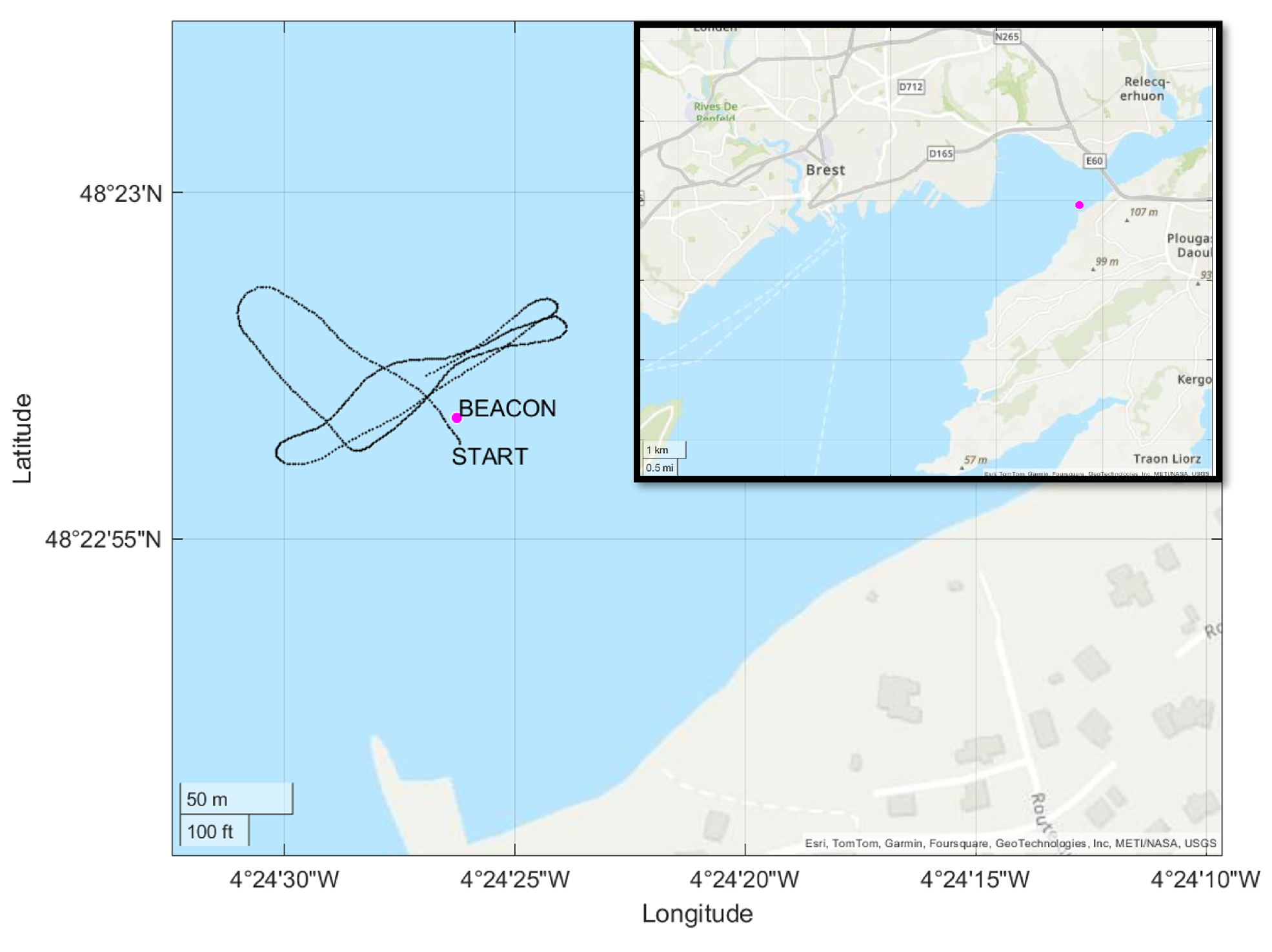
4.2.1. Description
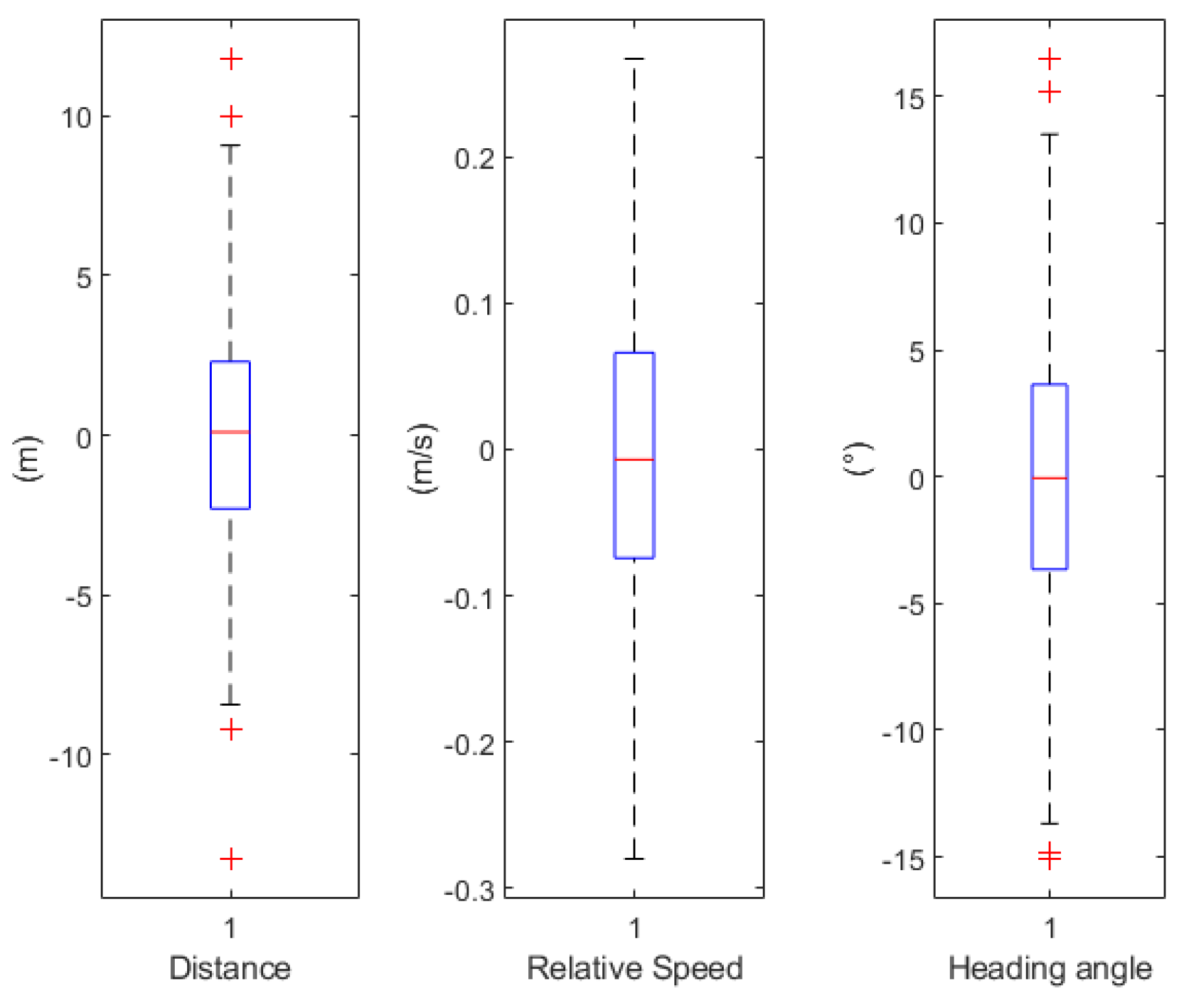
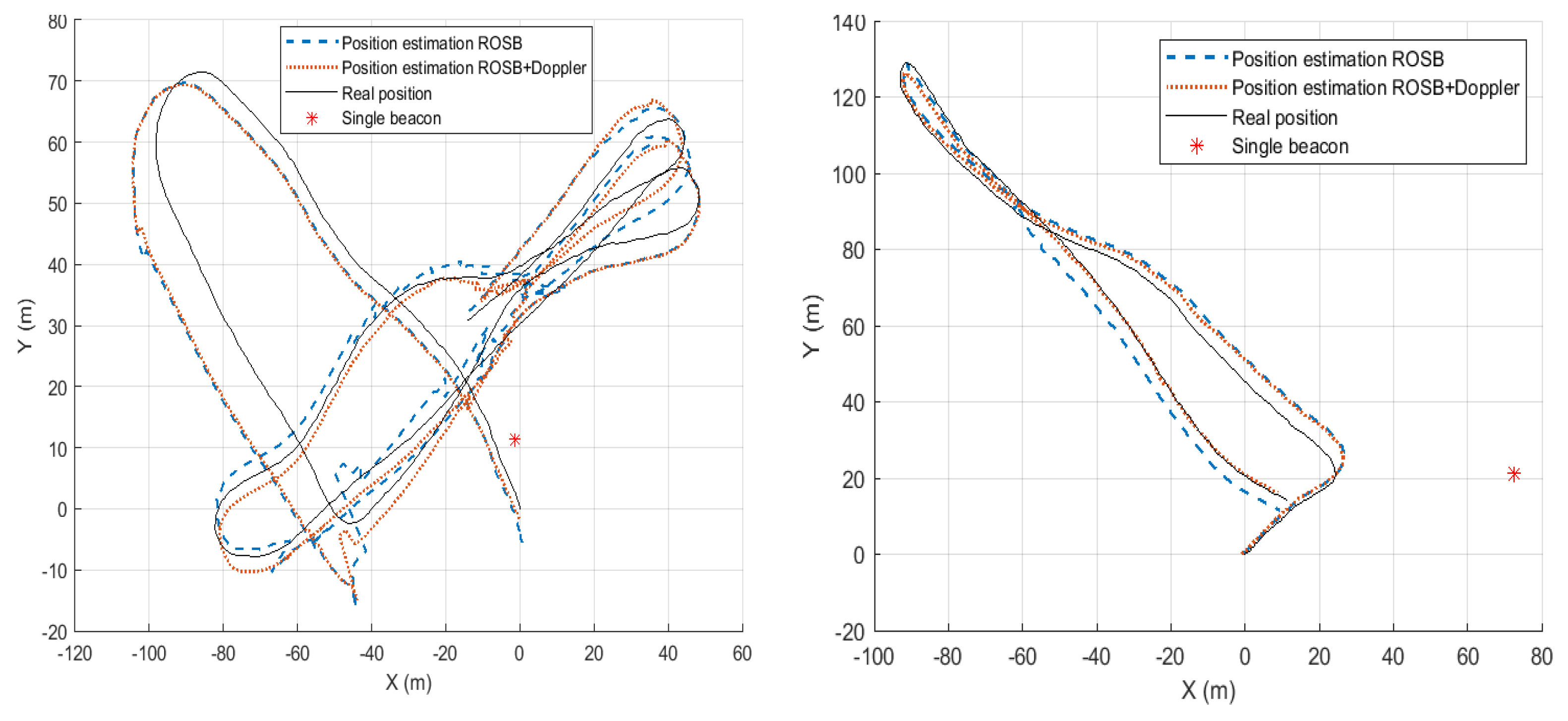
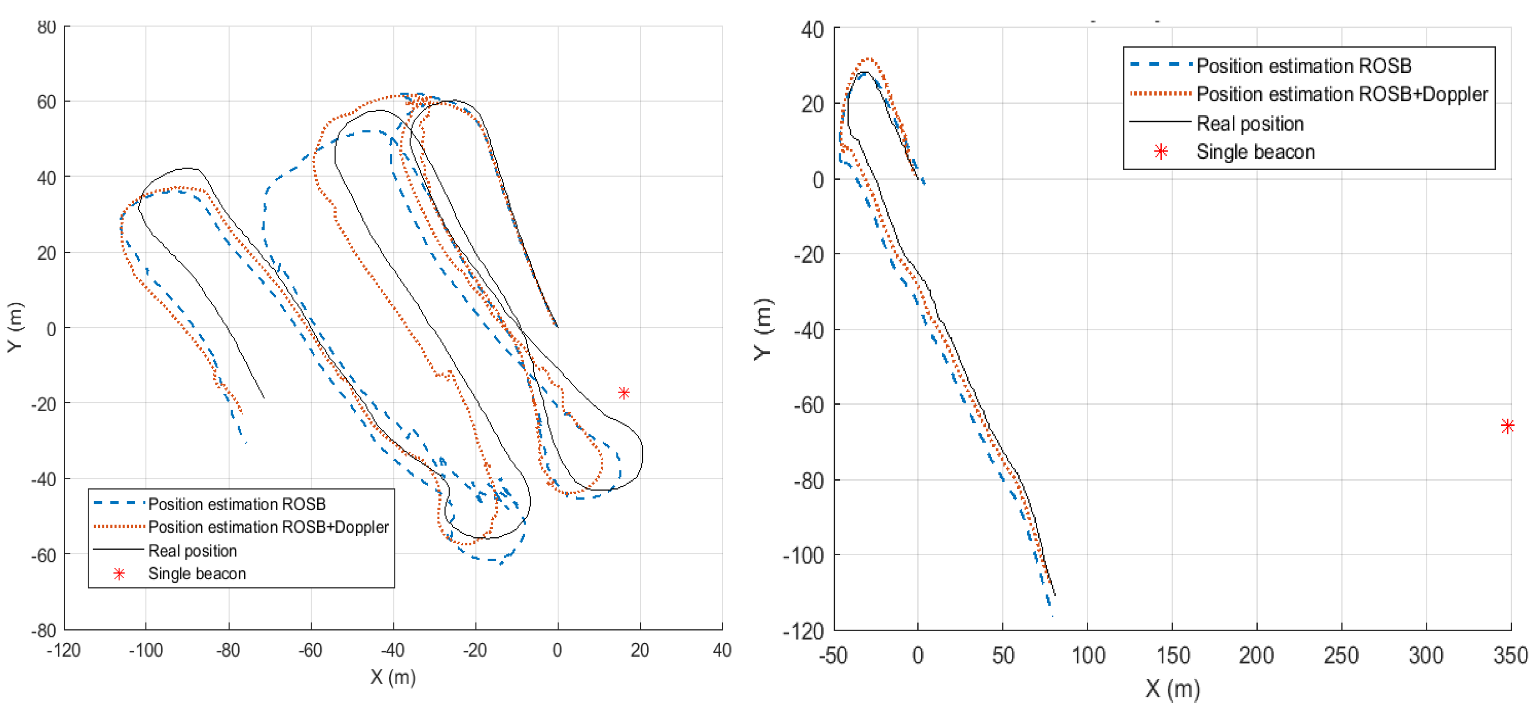
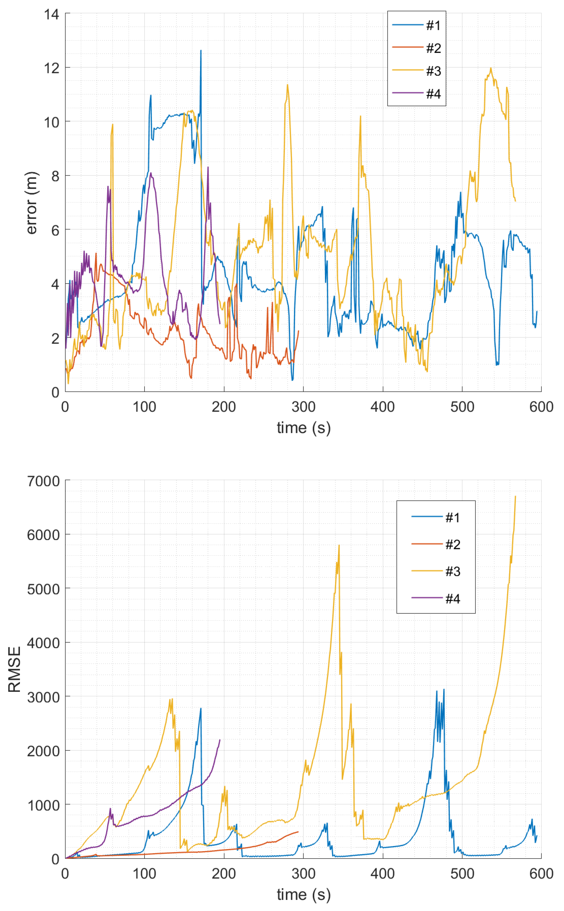
4.2.2. Experimental Results
- The sea current implies a boat drift, which impacts the heading angle, bearing angle and then relative speed . In fact, due to (13), we estimate only the forward speed and not the transverse speed.
- The bearing angle is not measured or estimated through UWA but through EKF linearity.
- Between each communication, the EKF only measures the heading angle .
5. Conclusions
Author Contributions
Funding
Informed Consent Statement
Data Availability Statement
Conflicts of Interest
References
- Ridao, P.; Carreras, M.; Ribas, D.; Sanz, P.J.; Oliver, G. Intervention AUVs: The Next Challenge. IFAC Proc. Vol. 2014, 47, 12146–12159. [Google Scholar] [CrossRef]
- González-García, J.; Gómez-Espinosa, A.; Cuan-Urquizo, E.; García-Valdovinos, L.G.; Salgado-Jiménez, T.; Cabello, J.A.E. Autonomous Underwater Vehicles: Localization, Navigation, and Communication for Collaborative Missions. Appl. Sci. 2020, 10, 1256. [Google Scholar] [CrossRef]
- Gussen, C.M.G.; Diniz, P.S.R.; Campos, M.L.R.; Martins, W.A.; Costa, F.M.; Gois, J.N. A Survey of Underwater Wireless Communication Technologies. J. Commun. Inf. Syst. 2016, 31, 242–255. [Google Scholar] [CrossRef]
- Stojanovic, M.; Beaujean, P.P.J. Acoustic Communication. In Springer Handbook of Ocean Engineering; Dhanak, M.R., Xiros, N.I., Eds.; Springer International Publishing: Cham, Switzerland, 2016; pp. 359–386. [Google Scholar] [CrossRef]
- Bouvet, P.; Auffret, Y.; Munck, D.; Pottier, A.; Janvresse, G.; Eustache, Y.; Tessot, P.; Bourdon, R. Experimentation of MIMO underwater acoustic communication in shallow water channel. In Proceedings of the OCEANS 2017—Aberdeen, Aberdeen, UK, 19–22 June 2017; pp. 1–6. [Google Scholar] [CrossRef]
- Eggen, T.H.; Baggeroer, A.B.; Preisig, J.C. Communication over Doppler spread channels. Part I: Channel and receiver presentation. IEEE J. Ocean. Eng. 2000, 25, 62–71. [Google Scholar] [CrossRef]
- Paull, L.; Saeedi, S.; Seto, M.; Li, H. AUV Navigation and Localization: A Review. IEEE J. Ocean. Eng. 2014, 39, 131–149. [Google Scholar] [CrossRef]
- Thomson, D. Acoustic Positioning Systems—The Hydrographic Society UK. Available online: https://www.yumpu.com/en/document/view/10350341/acoustic-positioning-systems-the-hydrographic-society-uk (accessed on 17 May 2022).
- Kaushik, A.; Singh, R.; Dayarathna, S.; Senanayake, R.; Di Renzo, M.; Dajer, M.; Ji, H.; Kim, Y.; Sciancalepore, V.; Zappone, A.; et al. Toward Integrated Sensing and Communications for 6G: Key Enabling Technologies, Standardization, and Challenges. IEEE Commun. Stand. Mag. 2024, 8, 52–59. [Google Scholar] [CrossRef]
- Masmitjà Rusiñol, I. Acoustic Underwater Target Tracking Methods Using Autonomous Vehicles. Ph.D. Thesis, Universitat Politècnica de Catalunya, Barcelona, Spain, 2020. [Google Scholar]
- Hunt, M.M.; Marquet, W.M.; Moller, D.A.; Peal, K.R.; Smith, W.; Spindel, R.C. An Acoustic Navigation System; Woods Hole Oceanographic Institution: Woods Hole, MA, USA, 1974. [Google Scholar]
- Yuan, M.; Li, Y.; Li, Y.; Pang, S.; Zhang, J. A fast way of single-beacon localization for AUVs. Appl. Ocean. Res. 2022, 119, 103037. [Google Scholar] [CrossRef]
- Casey, T.; Guimond, B.; Hu, J. Underwater Vehicle Positioning Based on Time of Arrival Measurements from a Single Beacon. In Proceedings of the OCEANS, Vancouver, BC, Canada, 29 September–4 October 2007; pp. 1–8, ISSN: 0197-7385. [Google Scholar] [CrossRef]
- Vickery, K. Acoustic positioning systems. A practical overview of current systems. In Proceedings of the 1998 Workshop on Autonomous Underwater Vehicles (Cat. No.98CH36290), Cambridge, MA, USA, 21 August 1998; pp. 5–17. [Google Scholar] [CrossRef]
- LaPointe, C.E.G. Virtual Long Baseline (VLBL) Autonomous Underwater Vehicle Navigation Using a Single Transponder. Mater’s Thesis, Massachusetts Institute of Technology, Cambridge, MA, USA, 2006; p. 94. [Google Scholar]
- iXblue. RAMSES Sparse-LBL Positioning System Datasheet. Available online: https://www.ixblue.com/wp-content/uploads/2021/12/ramses-lbl-transceiver-datasheet.pdf (accessed on 17 May 2022).
- Diamant, R.; Wolff, L.M.; Lampe, L. Location Tracking of Ocean-Current-Related Underwater Drifting Nodes Using Doppler Shift Measurements. IEEE J. Ocean. Eng. 2014, 40, 887–902. [Google Scholar] [CrossRef]
- Aubry, C.; Forjonel, P.; Bouvet, P.; Pottier, A.; Auffret, Y. On the use of Doppler-shift estimation for simultaneous underwater acoustic localization and communication. In Proceedings of the OCEANS 2019—Marseille, Marseille, France, 17–20 June 2019; pp. 1–5. [Google Scholar] [CrossRef]
- Garin, R.; Vanwynsberghe, C.; Forjonel, P.; Tomasi, B.; Bouvet, P.J. Simultaneous underwater acoustic localization and communication: An experimental study. In Proceedings of the OCEANS 2021: San Diego—Porto, San Diego, CA, USA, 20–23 September 2021; pp. 1–6. [Google Scholar] [CrossRef]
- Garin, R.; Bouvet, P.J.; Forjonel, P.; Tomasi, B. Sea experimentation of single beacon simultaneous localization and communication for AUV navigation. In Proceedings of the OCEANS 2023, Limerick, Ireland, 5–8 June 2023. [Google Scholar]
- UCNL Website. Available online: https://unavlab.com/en/o-nas/articles/myi-sdelali-samyiy-malenkiy-i-samyiy-deshevyiy-v-mire-gidroakusticheskiy-modem-uwave/ (accessed on 12 October 2024).
- Waterlinked Website. Available online: https://waterlinked.com/shop/modem-m16-186 (accessed on 12 October 2024).
- ArduPilot Website. Available online: https://ardupilot.org/ (accessed on 30 August 2024).
- Julier, S.; Uhlmann, J.; Durrant-Whyte, H. A new approach for filtering nonlinear systems. In Proceedings of the 1995 American Control Conference—ACC’95, Seattle, WA, USA, 21–23 June 1995; Volume 3, pp. 1628–1632. [Google Scholar] [CrossRef]
- Julier, S.; Uhlmann, J.; Durrant-Whyte, H. A new method for the nonlinear transformation of means and covariances in filters and estimators. IEEE Trans. Autom. Control. 2000, 45, 477–482. [Google Scholar] [CrossRef]


| Sensor | Standard Public Price | Measurement(s) |
|---|---|---|
| AHRS | EUR 1200 | Euler angles |
| Pressure | EUR 90 | Depth and temperature |
| GPS | EUR 20 | Surface position |
| UWA modem | from EUR 500 [21] to 2500 € [22] | Communication, Doppler, and range |
| Parameters | Description | Value |
|---|---|---|
| Mission duration | 1550 s | |
| Algorithm time step | 250 ms | |
| UWA communication period | s | |
| Number of simulation runs | 300 | |
| Beacon position | ||
| v | drone velocity | m/s |
| Mean Positioning Error (Outliers) in m | Variance of the Positioning Error | %etd Max | %etd Mean | |
|---|---|---|---|---|
| 3 s | 3.6054 (1) | 1.7549 | 0.5268 | 0.2281 |
| 6 s | 5.0440 (5) | 3.2143 | 0.5850 | 0.3152 |
| 9 s | 6.4518 (1) | 6.2173 | 0.7662 | 0.4032 |
| 12 s | 8.0853 (6) | 12.7455 | 1.0938 | 0.5053 |
| 15 s | 9.5457 (6) | 18.3823 | 1.3950 | 0.5966 |
| 20 s | 12.1322 (6) | 33.9161 | 1.7825 | 0.7583 |
| Mean Positioning Error (Outliers) in m with Proposed Method | Mean Positioning Error (Outliers) in m with ROSB | |
|---|---|---|
| 3 s | 3.6054 (1) | 4.5870 (4) |
| 6 s | 5.0440 (5) | 6.2255 (6) |
| 9 s | 6.4518 (1) | 7.7197 (5) |
| 12 s | 8.0853 (6) | 9.2462 (15) |
| 15 s | 9.5457 (6) | 10.6684 (10) |
| 20 s | 12.1322 (6) | 12.9695 (29) |
| Parameters | Description | Value |
|---|---|---|
| Algorithm time step | 1 s | |
| UWA communication period | 3 s | |
| Beacon position | ||
| UWA frame duration | 300 ms | |
| Pure-tone signal frequency | 20 kHz | |
| Data signal center frequency | 28 kHz | |
| Modulation speed | kHz | |
| B | Signal bandwidth | kHz |
| Sampling frequency | kHz |
| Trajectory | Mean Positioning Error in m with Proposed Method | Mean Positioning Error in m with ROSB Method |
|---|---|---|
| #1 ( = 600 s) | 4.6225 m | 5.4287 m |
| #2 ( = 300 s) | 2.1537 m | 2.9931 m |
| #3 ( = 600 s) | 5.0740 m | 8.6719 m |
| #4 ( = 200 s) | 4.2069 m | 6.2746 m |
| Trajectory | Traveled Distance in m | %etd Max | %etd Mean |
|---|---|---|---|
| #1 ( = 600 s) | 698.4989 | 1.7179 | 0.6617 |
| #2 ( = 300 s) | 353.3752 | 1.4149 | 0.6094 |
| #3 ( = 600 s) | 681.5850 | 1.7606 | 0.7444 |
| #4 ( = 200 s) | 190.5176 | 4.1990 | 2.2081 |
| Mean Positioning Error for #1 in m | Mean Positioning Error for #2 in m | Mean Positioning Error for #3 in m | Mean Positioning Error for #4 in m | |
|---|---|---|---|---|
| 3 s | 4.6225 | 2.1537 | 5.0740 | 4.2069 |
| 6 s | 5.0982 | 3.3472 | 7.1929 | 4.4613 |
| 9 s | 5.6782 | 3.3813 | 7.4395 | 5.0431 |
| 12 s | 6.0585 | 3.4354 | 8.4071 | 5.6932 |
| 15 s | DIV | 2.5071 | 8.2798 | 5.3535 |
| 18 s | 13.71 | 4.4618 | 9.3593 | 7.5195 |
Disclaimer/Publisher’s Note: The statements, opinions and data contained in all publications are solely those of the individual author(s) and contributor(s) and not of MDPI and/or the editor(s). MDPI and/or the editor(s) disclaim responsibility for any injury to people or property resulting from any ideas, methods, instructions or products referred to in the content. |
© 2024 by the authors. Licensee MDPI, Basel, Switzerland. This article is an open access article distributed under the terms and conditions of the Creative Commons Attribution (CC BY) license (https://creativecommons.org/licenses/by/4.0/).
Share and Cite
Garin, R.; Bouvet, P.-J.; Tomasi, B.; Forjonel, P.; Vanwynsberghe, C. A Low-Cost Communication-Based Autonomous Underwater Vehicle Positioning System. J. Mar. Sci. Eng. 2024, 12, 1964. https://doi.org/10.3390/jmse12111964
Garin R, Bouvet P-J, Tomasi B, Forjonel P, Vanwynsberghe C. A Low-Cost Communication-Based Autonomous Underwater Vehicle Positioning System. Journal of Marine Science and Engineering. 2024; 12(11):1964. https://doi.org/10.3390/jmse12111964
Chicago/Turabian StyleGarin, Raphaël, Pierre-Jean Bouvet, Beatrice Tomasi, Philippe Forjonel, and Charles Vanwynsberghe. 2024. "A Low-Cost Communication-Based Autonomous Underwater Vehicle Positioning System" Journal of Marine Science and Engineering 12, no. 11: 1964. https://doi.org/10.3390/jmse12111964
APA StyleGarin, R., Bouvet, P.-J., Tomasi, B., Forjonel, P., & Vanwynsberghe, C. (2024). A Low-Cost Communication-Based Autonomous Underwater Vehicle Positioning System. Journal of Marine Science and Engineering, 12(11), 1964. https://doi.org/10.3390/jmse12111964