Bearing Behavior of Large-Diameter Monopile Foundations of Offshore Wind Turbines in Weathered Residual Soil Seabeds

Abstract

The southeastern rock base sea area is the most abundant wind resource area, and it is also the mainstream construction site of offshore wind farms (OWFs) in China. The weathered residual soil is the main seabed component in the rock base area, which is the important bearing stratum of the offshore wind turbine foundation. Previous studies on the mechanical properties of seabed materials and bearing characteristics of the pile foundations in OWFs have mainly focused on the submarine soil-based seabed, resulting in a lack of direct reference for the construction of offshore wind power in the rocky seabed. Therefore, the mechanical properties of weathered residual soil and the bearing behaviors of monopile foundations are mainly investigated in this study. Firstly, dynamic triaxial tests are conducted on the weathered residual soil, and experiments analyze insight into the evolution law of the hysteresis curve, cumulative strain, and stiffness attenuation. Then, the horizontal loading behaviors of monopile foundations in residual soil are analyzed by numerical simulations; more critically, the service performances under wind and wave coupling loads are evaluated, which provide a direct theoretical basis for the construction and design of offshore wind turbine foundations in rock base seabeds.

1. Introduction

Wind energy is one of the most widely used renewable energy sources, and offshore wind power has the advantages of stable wind speed, abundant resources and no occupation of arable land compared with onshore wind energy [1,2]. In recent years, the rapid development of global offshore wind power has become an important means to promote industrial transformation and energy revolution [3,4]. A monopile foundation has the advantages of a simple, loaded, proven construction technology, and a high bearing capacity, and it is the most widely used foundation form on offshore wind farms [5]. Offshore wind turbine foundations last for a long time in complex marine environments, and the large-diameter monopile foundations are subjected to coupling loads combining wind, waves, current, and the overturning moment [6]. Horizontal load is an important control factor in the design of offshore wind turbine foundations [7,8,9,10]. Therefore, accurate evaluation of the horizontal bearing characteristics of large-diameter monopile foundations is necessary to ensure the safe installation and long-term normal service of offshore wind turbines [11,12,13].

Up until now, China has made remarkable achievements in the field of offshore wind power, with a cumulative installed capacity of 4.7 GW, which is the leading position in the world. With the rapid advancement of this field, the construction environment of offshore wind power projects is undergoing profound changes. The main construction sites of offshore wind farms have begun to shift from a sea area dominated by soft clay and silty seabed area to a weathered rock base sea area [14]. The weathered residual soil is the main component of the seabed in the rock-based area, and it is also the important stressed formation of the offshore wind turbine foundation. However, affected by sedimentation and weathering, the engineering geological properties and cyclic response of the weathering residual soil are obviously different from those of the marine soft clay and sandy soil [15]. At present, there have been abundant and systematic studies on the safety analysis and design methods of the large-diameter monopile foundation on a soil-based seabed, but hardly any research on monopile foundations on weathered rock seabeds has been carried out [16]. The design parameters of seabed materials and the p–y design method used for pile foundations in the existing regulations and studies are basically aimed at soft clay [17,18] and sandy seabeds [19,20,21] and cannot provide a direct reference and basis for the design and construction of monopile foundations in rock-based seabeds. Therefore, it is necessary to conduct a specific study on the mechanical properties of weathered residual soil materials and the horizontal bearing characteristics of large-diameter monopile pile foundations in a rock-based seabed.

The traditional analysis methods for determining the horizontal loading behavior of pile foundations can be divided into three types, i.e., the ultimate ground resistance method, the elastic ground reaction method, and the elastic–plastic composite ground reaction method (the p–y curve method). The p–y curve can simulate the pile–soil response under horizontal loads and is widely used in the horizontal loading analysis of pile foundations. In order to more accurately evaluate the horizontal bearing characteristics of large-diameter monopile foundations, many scholars have carried out many studies on the horizontal loading behavior of pile foundations through model tests [22], field tests [23], and numerical simulations [24,25], and many modified p–y curves for the large-diameter monopile foundation have been established. Long and Vanneste (1994) [26], Verdure et al. (2003) [27], and Peng et al. (2006) [28] have carried out some horizontal cyclic loaded in situ tests successively, and large amounts of precious data were obtained, including information on the displacement and bending moment. More studies about the horizontal loading behavior of pile foundations have been carried out through physical modeling experiments and numerical simulations. For example, Byrne et.al. (2010) conducted model tests of a rigid pile under horizontal unidirectional and bidirectional cyclic loads and analyzed the effects of cyclic load ratio and loading times on cumulative deformation [29]. Lesny and Wiemann (2005) used ABAQUS v6.14 software to simulate the horizontal loading behaviors of large-diameter monopile foundations and modified the initial reaction modulus of the traditional p–y curve method [30]. The above studies are of great significance to the analysis of the horizontal loading behavior of large-diameter monopile foundations in soil seabeds and also provide an important theoretical basis and method support for the study of the horizontal loading characteristics of large-diameter monopile foundations in weathered residual soil.

Therefore, weathered residual soil, as a special seabed material, is reviewed as the study object, and the mechanical properties of weathered residual soil and the bearing behaviors of pile foundations in weathered residual soil are mainly investigated by dynamic triaxial tests and numerical simulations. Firstly, dynamic triaxial tests are carried out for the weathered residual soil, and experiments analyze the evolution law of the hysteresis curve, cumulative strain, and stiffness attenuation. Then, the horizontal loading behaviors of monopile foundations in residual soil are analyzed by numerical simulation and, more critically, the service performances under wind and wave coupling loads are evaluated, which provide a direct theoretical basis for the construction and design of offshore wind turbine foundations in a rock-based seabed.

2. Soil Sample and Test Method

2.1. Residual Soil Sample

The testing soil samples were taken from an offshore wind farm in Pingtan City, Fujian Province, and the sampling depth is 2–15 m below the surface, which is mainly weathered granite residual soil. To secure the natural state and reduce additional disturbance, the static pressure sampling method of the drilling rig is used to bring the soil sample out through the bulldozer by applying pressure, which is then immediately wrapped in a plastic tube and sealed with tape and wax, and transported back to the laboratory through a wooden box with cushioned foam for proper preservation. According to the geotechnical test procedure, a series of necessary physical and mechanical properties tests were carried out on the weathered residual soil samples. The specific gravity method was used to test the specific gravity of the weathered residual soil samples, and the drying method was used to test the natural moisture content. The liquid–plastic limit combined measurement method was used to test the liquid–plastic limit index of the samples, and the sieve analysis method and the densimeter method were used to determine the particle size curve. The basic physical properties of the weathered residual soil are shown in Table 1.

Table 1. Basic physical properties of weathered residual soil.

Natural Density (g/cm3)	Water Content (%)	Liquid Limit (%)	Plastic Limit (%)	Plasticity Index	Uniformity Coefficient Cu	Curvature Coefficient Cc
1.90	31.36	37.05	22.98	14.07	100.20	0.18

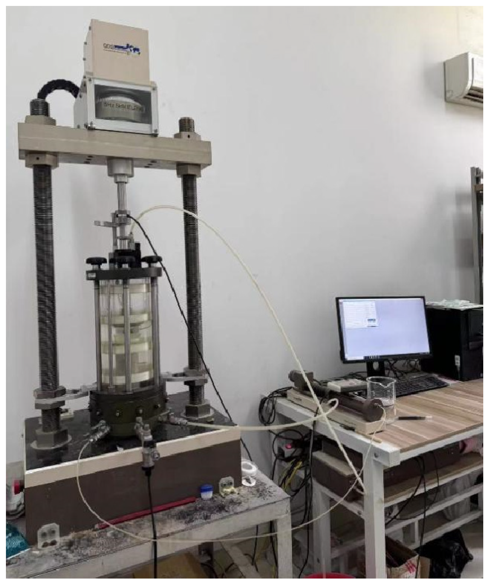
2.2. Testing Apparatus and Procedure

The instrumentation used in this paper is the GDS Dynamic Triaxial Test System (ELDyn) from the UK, as shown in Figure 1, which consists of an axial pressure loading module, a peripheral pressure loading module, a pressure chamber, a counter-pressure controller, a data acquisition module, and the GDSLab operating software (v2.5.0). Under the strain-controlled mechanism, the test system can implement a maximum axial dynamic load of ±5 kN, a maximum frequency of 20 Hz, and a maximum pressure of 1000 kPa. This test system can meet the requirements of different test conditions and test scenarios. Cylindrical soil samples were prepared with a diameter of 50 mm and a height of 100 mm. As the tested soil showed low permeability, the dynamic tests were carried out under undrained conditions. The vacuum saturation method was adopted as the only saturation method in this study, and the saturation of soil samples was up to the test requirement after 24 h vacuum saturation. The samples were submerged in a vacuum saturator after cutting and were placed on the apparatus immediately after the completion of saturation for the experiments.

Figure 1. British GDS dynamic triaxial test system.

Static triaxial tests were carried out on the weathered residual soil under three level confining pressures 100 kPa, 200 kPa and 300 kPa. Dynamic triaxial tests were carried out on the three levels of confining pressures, i.e., 40 kPa, 55 kPa and 70 kPa. The cyclic axial load is controlled by the cyclic stress ratio (CSR), and the dynamic triaxial test schedule of weathered residual soil is illustrated in Table 2.

Table 2. Dynamic triaxial test schedule of weathered residual soil.

Test Number	Confining Pressure (kPa)	CSR
RS-1~4	40	0.4, 0.5, 0.55, 0.6
RS-5~8	55	0.4, 0.45, 0.5, 0.6
RS-9~12	70	0.4, 0.45, 0.5, 0.6

3. Mechanical Properties of Weathered Residual Soil

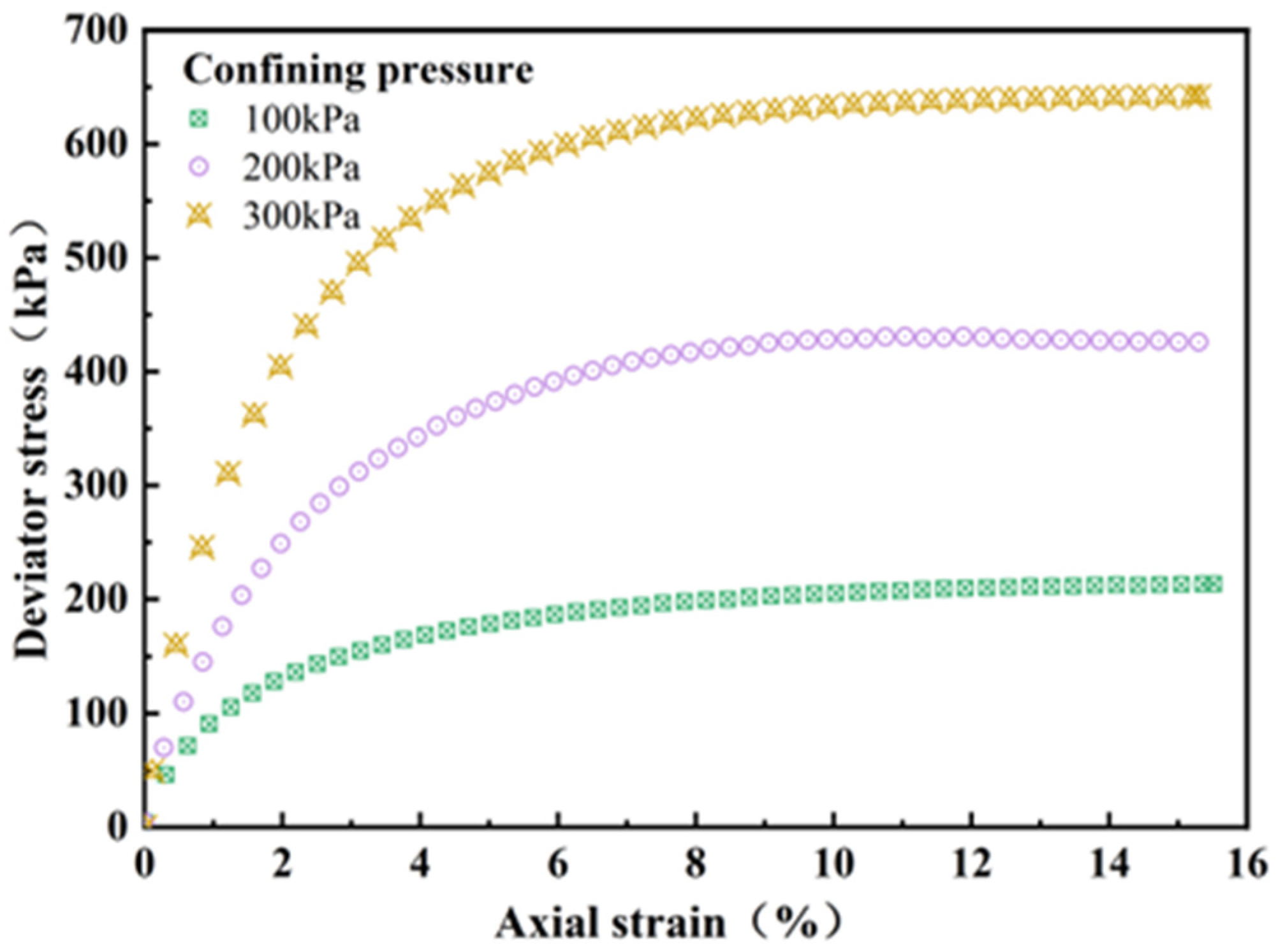
3.1. Static Testing Results

The effective cohesion of the weathered residual granite is 6.57 kPa and the effective internal friction angle is 34.77°. The stress–strain curves of the testing soil samples under different confining pressures are illustrated in Figure 2. The deviational stress of the soil samples accumulates continuously with the increase in axial strain, and the stress–strain curves first increase linearly, then slowly grow non-linearly, and eventually flatten out. When the axial strain is 0–3%, the soil specimen is in the elastic deformation period, and the curve increases linearly. When the axial strain is 3–6%, the sample is in the elastoplastic deformation stage, and the internal structure of the soil sample begins to fail irreversibly, and the curve grows nonlinear. The strain hardening occurs when the axial strain is greater than 6%, and the specimen gradually loses its bearing capacity and finally in the failure state.

Figure 2. Stress–strain curve in the static triaxial test.

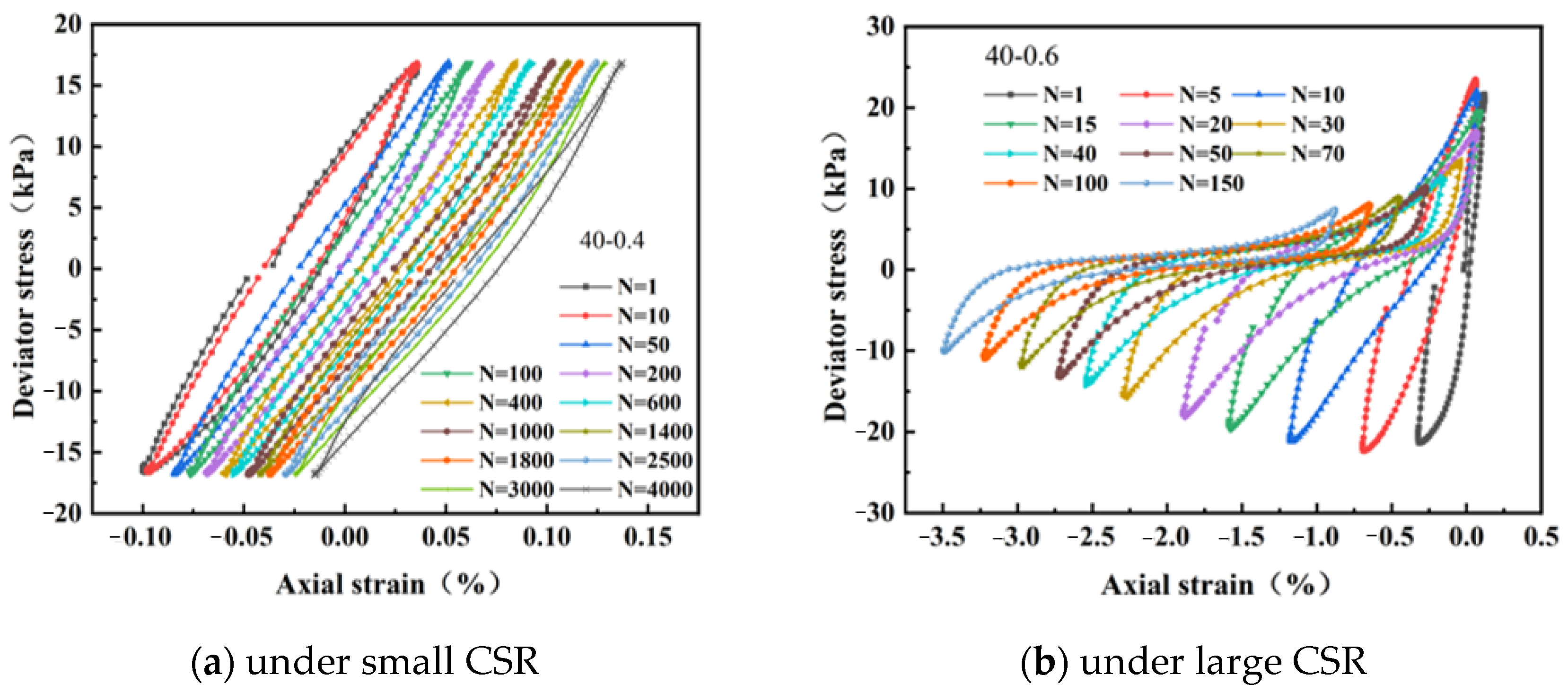
3.2. Evolution of Hysteresis Curve of Weathered Residual Soil

Figure 3 shows the hysteresis curves of weathered residual soil samples at 40 kPa confining pressure. When the cyclic stress ratio (CSR) is relatively small, the shape and position of hysteresis curves of the soil sample basically do not change significantly with the increase in the cycle numbers, and the cumulative strain is small. Under cyclic loads with small CSR, the soil sample is still in a stable state, and the morphology of the soil sample is basically unchanged, which indicates that the internal connections of soil particles do not change greatly. As shown in Figure 3a, the areas of hysteresis curves in each cycle are roughly same, which means the dissipated energy after each cycle is almost the same.

Figure 3. Stress–strain curve of the dynamic triaxial test.

When the CSR is relatively large, the hysteresis loops gradually change with the increase in cycle numbers. The hysteretic loops rotate toward the direction of axial strain accumulation and change from a relatively regular spindle shape to other shapes. The morphology of the soil sample is crushed, and the internal positions of soil particles change obviously. Meanwhile, under the same confining pressure, the larger the CSR is, the faster the plastic deformation accumulates, as shown in Figure 3b.

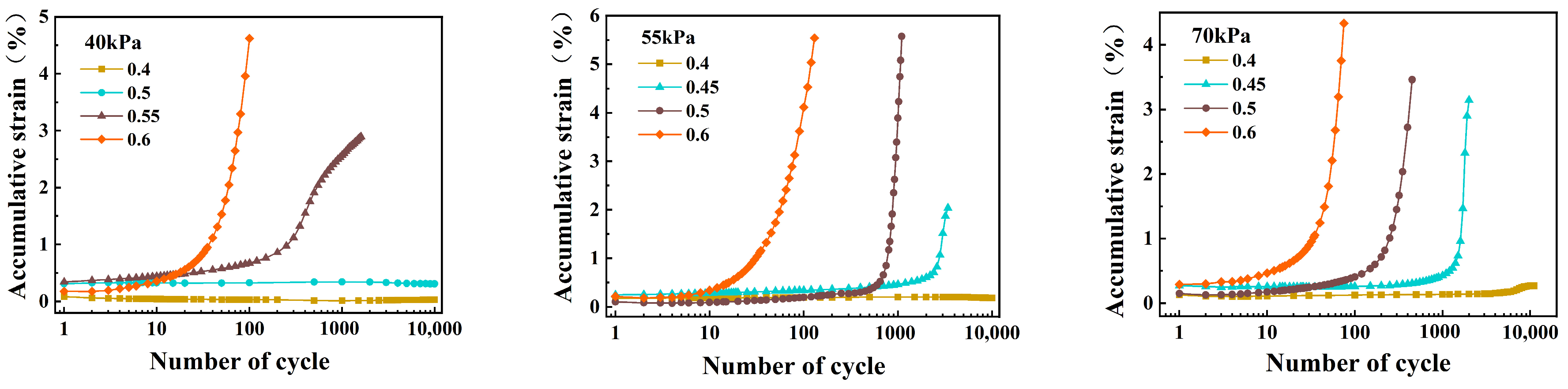
3.3. Development Law of Cumulative Strain

Figure 4 shows the relationship between the accumulative strain and the number of cyclic loads under different dynamic stress amplitudes with three levels of confining pressure. When the CSR is relatively small, the cumulative strain generated by the soil under the action of the cyclic load is small, and the cumulative strain increases slightly with the increase in the number of cycles but is at a low level as a whole. At this time, the appearance of the sample is almost unchanged and can withstand long-term low-strength cyclic loading. When the CSR is relatively large, the cumulative strain of the sample first increases slowly and then increases rapidly after a certain number of cycles. Under the action of high-strength dynamic load, the internal structure of the soil is destroyed, resulting in the axial flattening of the external shape. The larger the CSR, the faster the cumulative strain curve develops, and the more prone to deformation and failure of the sample.

Figure 4. Development law of accumulative strain.

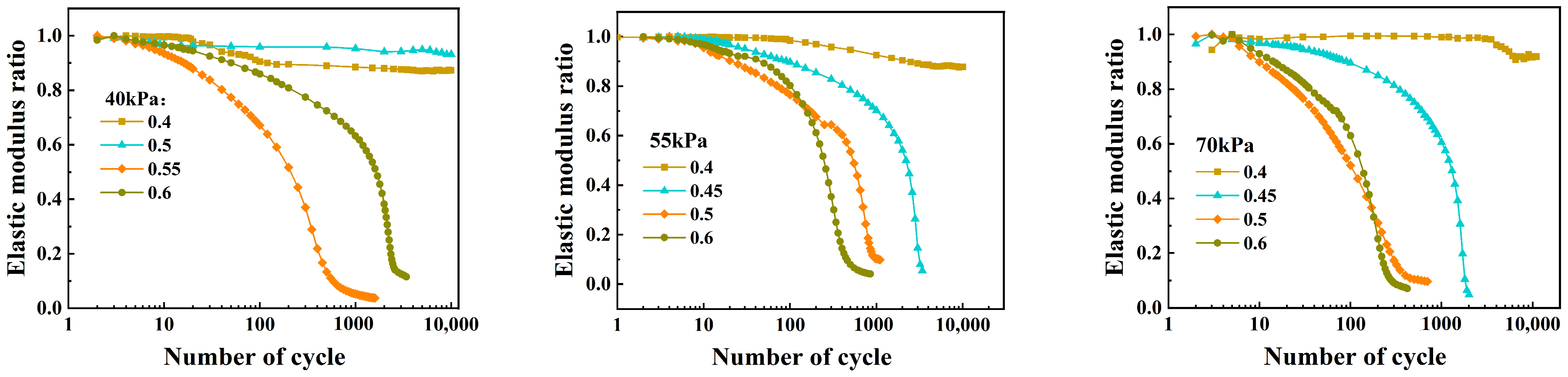
3.4. Development Law of Dynamic Elastic Modulus

Figure 5 shows the development law of dynamic elastic modulus of weathered residual soil under different confining pressures. It can be seen from Figure 5 that the attenuation ratio of dynamic elastic modulus under small CSR decreases slightly with the increase in the cycle number. After the number of cyclic loads reaches a certain number, the dynamic elastic modulus maintains a relatively stable level and the stiffness maintains a large value, indicating that the strength of the soil sample can resist the influence of the cyclic loads and maintain a relatively stable state.

Figure 5. Development law of dynamic elastic modulus ratio.

When the CSR is relatively large, the dynamic elastic modulus ratios of the soil sample rapidly decay to near 0 with the increase in the cycle number. More critically, the greater the CSR, the more drastic the modulus decay. Under large cyclic loads, soil samples are unable to withstand high-strength cyclic loads and gradually lose the bearing capacity. The large CSR leads to the obvious attenuation of dynamic elastic modulus under the same confining pressure.

4. Finite Element Numerical Model of Pile–Soil Interaction

There are various foundation forms for offshore wind turbines, and a monopile foundation is the most widely used in offshore wind farms. The monopile foundation is long-term in complex marine environments and is subjected to the coupling loads combining the wind and wave loads. The horizontal load is the main loaded mode of offshore wind turbine foundation. Therefore, the 3D numerical model of offshore wind turbine monopile foundation in weathered residual soil is established in the study, as shown in Figure 6, and the horizontal bearing characteristics of the monopile foundation are analyzed. The size of the seabed foundation is 100 m in diameter and 60 m in height, and the numerical model of the monopile foundation is 5 m in diameter and 38 m in length (30 m in pile depth and 8 m in pile length above the mud surface). The monopile foundation is equivalent to a solid steel pile, and the linear elastic constitutive model is adopted. The Mohr–Coulomb constitutive model is adopted for the weathered residual soil seabed, and the parameters of the monopile foundation and seabed material are illustrated in Table 3. In order to more clearly describe and compare the bearing characteristics of monopile foundations in weathered residual soil, the horizontally loaded behavior of monopile foundations in soft clay is also conducted in the study. For the convenience of comparison and description, the soft clay is recorded as soil A and the weathered residual soil is recorded as soil B.

Figure 6. Finite element calculation model of pile–soil interaction.

Table 3. Material parameters in the numerical model.

Assembly Unit	Elasticity Modulus (kPa)	Cohesive Force ${\mathit{c}}^{\prime }$ (kPa)	Internal Friction Angle ${\mathit{\phi }}^{\prime }$ (°)	Poisson Ratio	Weight (kN/m3)
Monopile foundation	2.1 × 108	—	—	0.24	—
Soft clay seabed	9300	11.88	30.94	0.32	16.8
Weathered residual seabed	17,500	6.57	34.77	0.3	19

In the numerical model, the C3D8 elements are used for foundation and monopile components, and the mesh size of the pile body and soil surrounding the pile is 0.5 m, and the mesh size of the soil under the pile bottom is 1 m. The contact mode between pile and soil is hard to contact in the normal direction and friction contact in the tangential direction. The contact friction coefficient of pile–soil interaction is determined by the formula $k=\mathit{tan}\left(0.75{\phi }^{\prime }\right)$, meanwhile, the coefficient k in soft clay (soil A) is 0.42, and that in weathered residual soil (soil B) is 0.49. The displacements in the x, y and z directions of the numerical model are constrained at the bottom of the soil, the displacements in the x and y directions are constrained at the side, and no constraints are set at the top surface.

5. Bearing Characteristics of Monopile Foundation

5.1. Horizontal Load–Displacement Response

Based on the above-established numerical model of pile–soil interaction, the displacement control method is used to obtain the horizontal load–displacement response curve of the pile head. A series of horizontal displacements are applied to the pile top, and the corresponding horizontal loads of the pile top are extracted. The horizontal load–displacement response curve of the pile head is illustrated in Figure 7.

Figure 7. Horizontal load–displacement of monopile foundation.

It can be seen from Figure 7 that the horizontal load of the monopile foundation increases with the increase in horizontal displacement whether in weathered residual soil (soil B) and soft clay (soil A) and the load–displacement response curve undergoes the linear to a nonlinear relationship. At the initial loading stage of horizontal load, the pile–soil system is in the elastic deformation stage, and the relationship between horizontal load and displacement is linear. With the increase in horizontal load, plastic deformations occur on the soil around the monopile foundation, and the curvature of the load–displacement response increases slowly. The relationship between horizontal load and displacement becomes nonlinear, and the pile–soil system is in the plastic failure stage.

By comparing the bearing characteristics of monopile foundation in A and soil B seabed, the horizontal load–displacement response of pile head in soil B is always above that in soil A, and the ultimate bearing capacities of monopile foundation in weathered residual soil and soft clay seabed are 21.3 and 14.4 MN, respectively. The initial stiffness of monopile foundation in in weathered residual soil is 44.28 MN/m, and that is soft clay is 26.15 MN/m. The bearing capacities of monopile foundations in weathered residual soil are larger than those of soft clay.

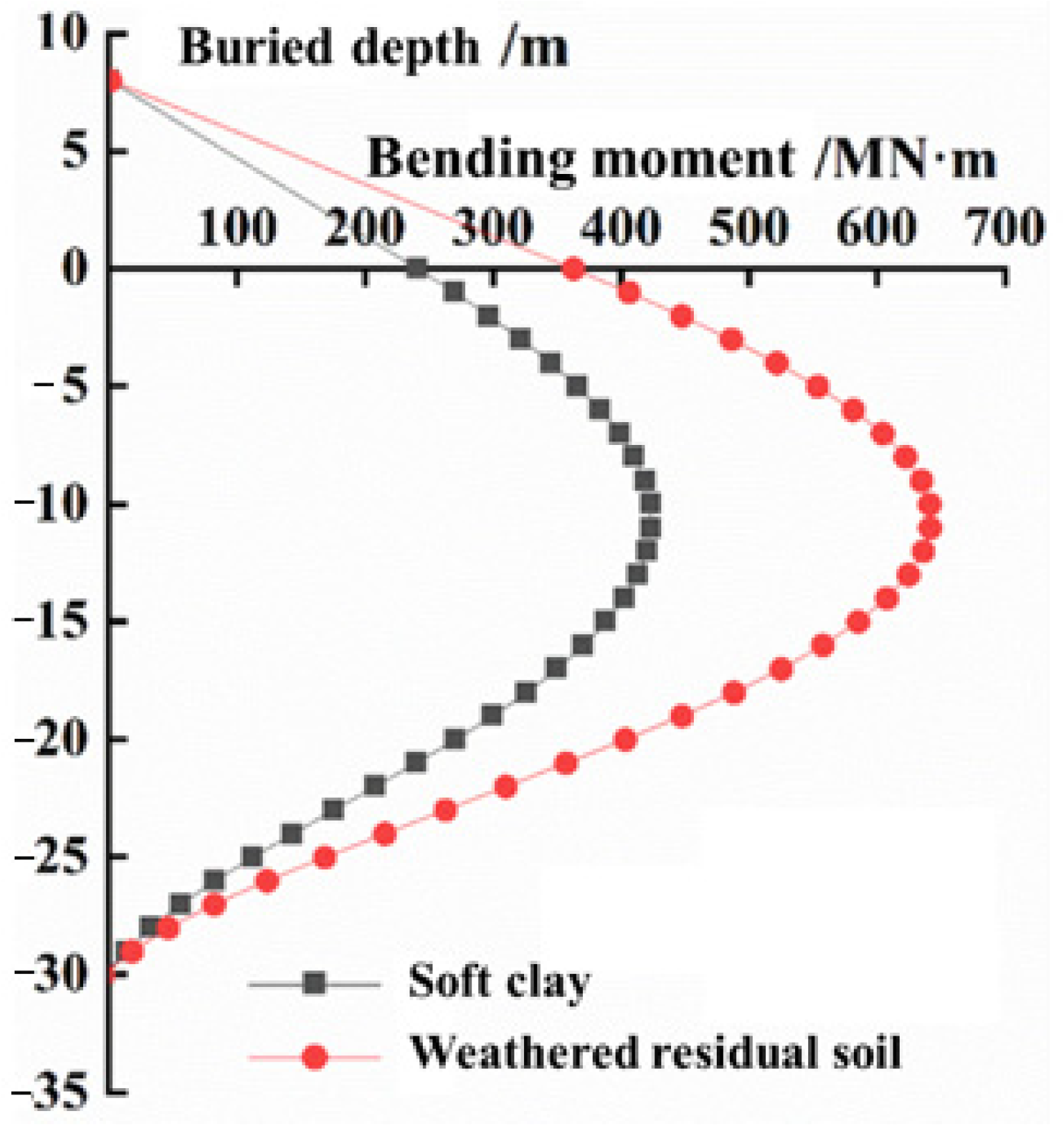
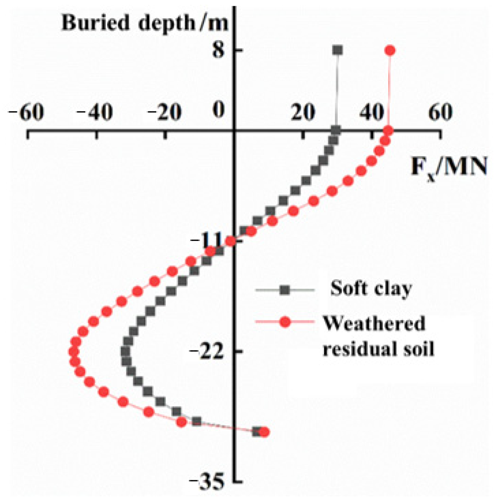
5.2. Bending Moment and Shear Force Response

Figure 8 shows the response of the bending moment of the pile body with burial depth at the 3 m horizontal displacement imposed on the pile head. It can be seen that the pile bending moment firstly increases with the burial depth, then gradually decreases after reaching the peak value; meanwhile, the maximum value of bending moment occurs at the 11 m burial depth. It is also noted that the bending moment of the pile body in soil A is obviously greater than that in soil A. The maximum bending moment in soil A is 423 MN·m, and the maximum bending moment in soil B is 641 MN·m, that means that the horizontal resistance of soil B is greater than that in soil A, and greater bending moment is needed to make the pile–soil structure failure in soil B.

Figure 8. Bending moment with burial depth.

Figure 9 illustrates the response of the shear force with the pile burial depth at the 3 m horizontal displacement imposed on the pile head, and the negative value of shear force in the figure only represents the opposite direction. The changing trend of the shear force of monopile foundation in two soil seabeds is the same. The shear force gradually decreases from 0–11 m burial depth and changes direction at −11 m burial depth, which corresponds to the maximum bending moment of the pile. The absolute value of shear force under 11 m burial depth increases firstly and then decreases, and reaches the maximum value at 22 m burial depth, which corresponds to the rotation point of the pile. Compared with the two working conditions, the shear force value of the pile body in soil B is greater than in soil A, and greater shear force is required to make the deformation failure of the pile–soil structure in soil B.

Figure 9. Shear force with burial depth.

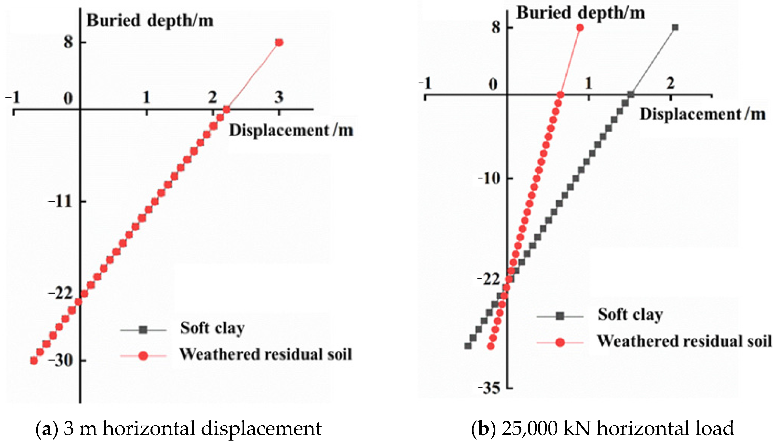
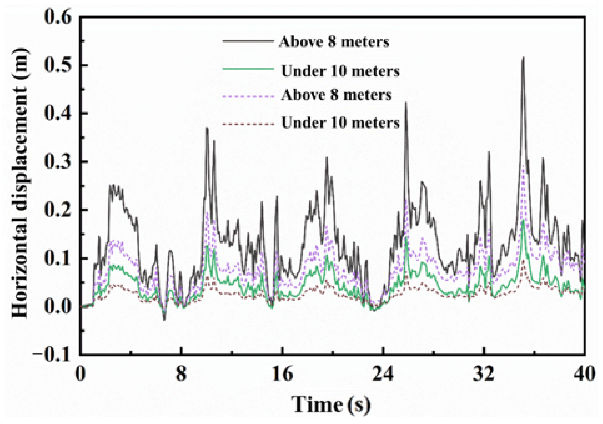
5.3. Horizontal Displacement of Pile Body with Burial Depth

The monopile foundations in weathered residual soil and soft clay belong to the rigid pile in the study, and the horizontal displacements of the pile body at different burial depths are illustrated in Figure 10. With an imposed 3 m horizontal displacement on the pile head, the pile displacement–burial depth curves of two soil seabeds are completely consistent, as shown in Figure 10a, and the monopile foundation rotates around a point at about 22 m burial depth, which is defined as the rotation center. The pile body rotates to the right above the rotation center and rotates to the left below the rotation center. Meanwhile, the rotation center is 2/3 of burial depth (L), and this study’s conclusions have been obtained in previous studies.

Figure 10. Pile horizontal displacement–burial depth curve.

Figure 10b shows the response of pile displacement with burial depth in two soil seabed under 25,000 kN horizontal load. It is noted that the overall horizontal displacement of the pile body in soil A is much larger than that in soil B, indicating that the bearing capacity of soil B is larger than soil B. At the same time, the monopile foundation rotates around the rotation center at about 22 m burial depth, where the pile foundation has no horizontal deformation, as characterized by the rigid pile.

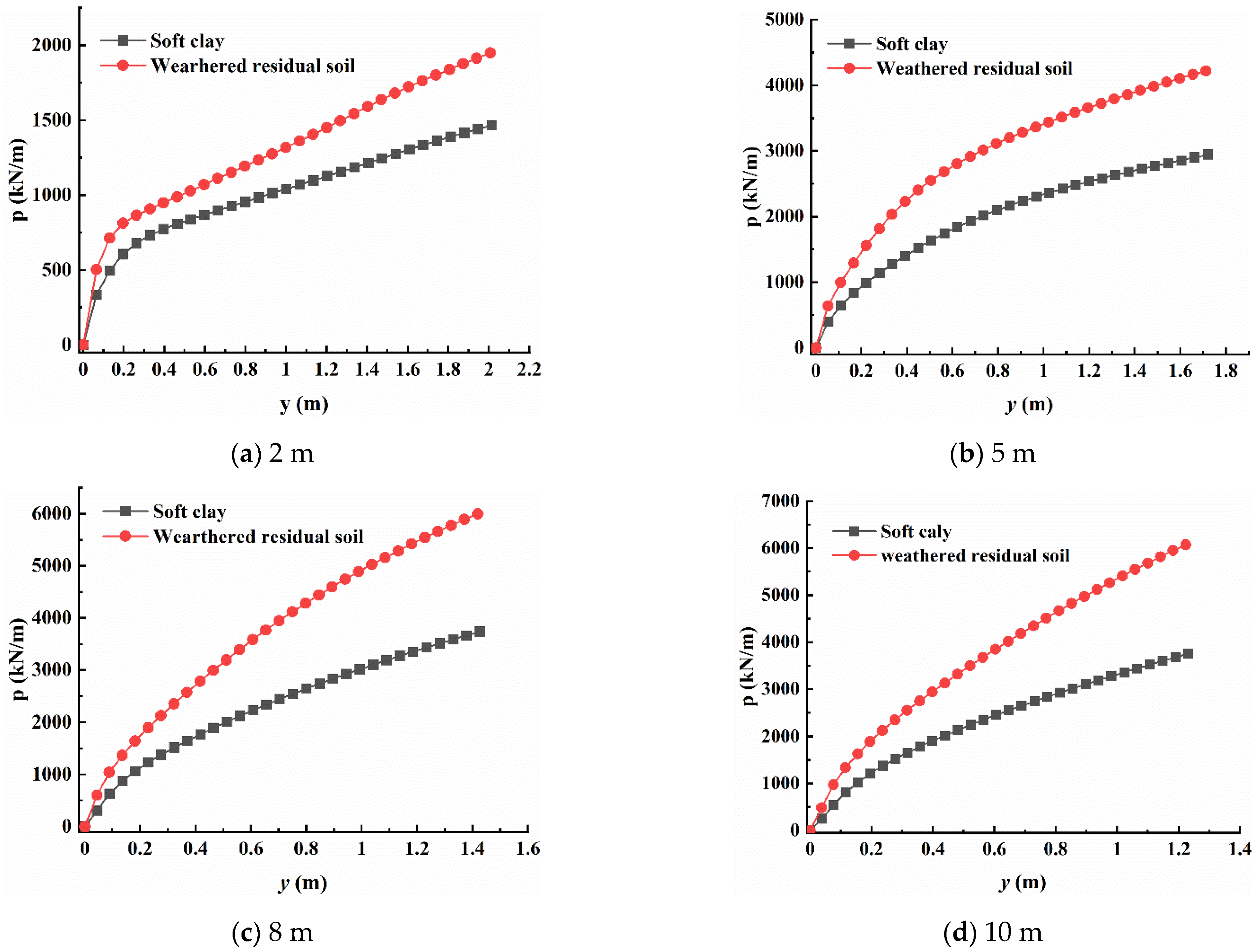
5.4. p–y Curve Response

The soil reaction of the soil around the pile is extracted after the 3 m horizontal displacement imposed on the pile head, and Figure 11 shows the distribution curve of soil resistance with the burial depth, where the positive and negative values of soil resistance only indicate the load direction. It is noted that the seabed with a 0–22 m burial depth provides the left-directed resistance, and soil resistance gradually increases and then decreases with the increase in the burial depth. Meanwhile, the ultimate soil resistances reach the maximum at about 11 m burial depth in two soil seabed, and there is no resistance at 22 m of the burial depth, which indicates that there is no lateral displacement of the monopile foundation at a 22 m burial depth. Below a 22 m burial depth, the soil around the monopile foundation provides right-directed resistance, and the soil resistance increases with the increase in the burial depth, which corresponds to the pile displacement distribution with the burial depth in Section 5.3.

Figure 11. Distribution of soil resistance along burial depth of pile body.

Figure 12 shows p–y curves at different burial depths. The soil resistance increases with the increase in horizontal displacement, and the p–y curves increase linearly and then nonlinear slowly. Under the same load conditions, the p–y curve of soft clay seabed is below that in the weathered residual soil, indicating that weathered residual soil can produce greater resistance to prevent the deformation of the monopile foundation.

Figure 12. p–y curves at different burial depths.

6. Long-Term Service Performance of Monopile Foundation

The monopile foundation of offshore wind turbines is subjected to the cyclic loads combining the wind and wave, and the coupling loads are imposed on the established numerical mode to investigate the long-term service performance.

6.1. Calculation and Application Method of Wind and Wave Loads

6.1.1. Wind Load Calculation

The wind loads applied to the tower and blade of offshore wind turbines can be divided into the average wind and the fluctuating wind, and the specific manifestations of wind speed acting on the structure are as follows:

$$V\left(z,t\right)=\overline{v}\left(z\right)+v\left(z,t\right)$$

(1)

where $\overline{v}\left(z\right)$ is the average wind speed, which does not change with time in a certain period of time. $v\left(z,t\right)$ is the fluctuating wind speed, and changes with time evolution according to random law.

Among, the change law of the average wind speed with height can be expressed by exponential function (Formula (2)), and the average wind speed at any height can be calculated according to the reference height and average wind speed in the standard.

$${\displaystyle \frac{\overline{v}\left(z\right)}{\overline{v_b}}}={\left({\displaystyle \frac{z}{z_b}}\right)}^{\alpha }$$

(2)

where $z \mathrm{a}\mathrm{n}\mathrm{d} \overline{v}\left(z\right)$ are the calculated height and the average wind speed at any height. $z_b \mathrm{a}\mathrm{n}\mathrm{d} \overline{v_b}$ are the reference height and the corresponding average wind speed recommended in the standard. $\alpha$ is the ground roughness index, which is valued as 0.12, due to the surface type being offshore sea or island in the study. According to the wind energy resource report and the distribution map of wind energy resources in the coastal region, the average wind speed at a height of 10 m is 37.5 m/s in the study.

Fluctuating wind speed is characterized by a large amount of randomness, and the wind speed spectra with similar statistical characteristics are generally used for the simulation of the fluctuating wind speed. Davenport’s horizontal pulsating wind spectrum is used in the study, and the computational formula is given below.

$$\left\{\begin{array}{c}{S}_v\left(n\right)={\overline{v_{10}}}^2{\displaystyle \frac{4k{x}^2}{n{\left(1+x^2\right)}^{4/3}}}\\ x=1200n/\overline{v_{10}}\end{array}\right.$$

(3)

where $S_v\left(n\right)$ is the power spectrum of the fluctuating wind speed, n is the fluctuating wind frequency, Hz. k is the ground roughness coefficient, $\overline{v_{10}}$ is the average wind speed at 10 m height, m/s. The time history and power spectrum of the fluctuating wind speed with a 40 s period at 10 m height can be obtained by MATLAB (https://ww2.mathworks.cn/products/matlab.html?s_tid=hp_ff_p_matlab), as shown in Figure 13.

Figure 13. Fluctuating wind speed time history curve and power spectrum. (a) Time history curve of fluctuating wind speed at 10 m height. (b) Power spectrum for simulating wind speed.

After the average wind speed and fluctuating wind speed are obtained, the total wind speed at each height can be calculated according to the Formulas (1) and (2), and the wind load actioning different heights of the offshore wind turbine can be calculated as Formula (4). The time history curve of total bending moment acting on the mud surface raised by the wind loads actioning on offshore wind turbines, and the shapes and dimensions of the tower and blades are determined from the basic component parameters of EN-136/4 MW turbine, which is also illustrated in Table 4.

$$F_w=0.5\rho {V\left(z,t\right)}^{2}cA$$

(4)

where $F_w$ is wind load, $\rho$ is the air density, 1.225 kg/m³, $V\left(z,t\right)$ is the wind speed at Zm height above the water level, m/s, c is the shape factor, which can be 0.5. A is the projected area of the tower perpendicular to the wind direction, m².

Table 4. Basic component parameters of EN-136/4 MW wind turbine.

Wind Turbine Parts	Offshore Wind Turbine Size (m)				Weight (t)
	Length	Width	High	External Diameter
Cabin	13.96	4.33	5.54	-	145
Hub	4.07	5.19	5.08	-	100
Blade	63.44	4.2	3.39	-	-
Up end of tower	-	-	29.9	3.66–4.19	62.76
Middle end of tower	-	-	27.77	4.19–4.63	90.97
Lower end of tower	-	-	18.33	4.63–5.00	83.42

6.1.2. Wave Load Calculation

The Airy wave theory has the advantages of simple principles and convenient calculation and has been widely used in marine structural engineering. Therefore, the Airy wave theory is used to calculate the wave load in the study, and calculation parameters are referenced in the study [31]. The calculation formulas of horizontal velocity $u$ and acceleration ${\displaystyle \frac{\partial \mathrm{u}}{\partial \mathrm{t}}}$ in Airy wave theory are as follows.

$$u={\displaystyle \frac{H\omega \cosh k(d+z)}{2\sinh kd}}\cos \theta$$

(5)

$${\displaystyle \frac{\partial u}{\partial t}}={\displaystyle \frac{H{\omega }^2\cosh k(d+z)}{\sinh kd}}\sin \theta$$

(6)

where the forward direction of the wave is defined as the X-axis and the vertical upward direction of the pile center is the Z-axis. $\theta =kx-\omega t$, $k=2\mathsf{\pi }/\mathrm{L}$. H is the wave height, which is 6.54 m in the study. $\omega$ is the circular frequency, Hz. d is the water depth, m. T is the wave period, which is 8 s in the study.

Wave motion parameters are determined by the Airy wave theory, and the Morison equation is used to calculate the wave load distributed on a monopile foundation, as in the formula given below.

$$df=0.5\ast {\displaystyle \frac{\gamma }{g}}{C}_D{D}_u\left|u\right|d_z+{\displaystyle \frac{\gamma }{g}}{C}_{M}A{\displaystyle \frac{\partial u}{\partial t}}{d}_z$$

(7)

where $C_D$ is the velocity force coefficient, $C_M$ is the mass force coefficient, D is the pile diameter, m. $d_z$ is the unit pile length, m. A is the cross-sectional area of the monopile foundation ${\mathrm{m}}^2$.

6.1.3. Combining Wind and Wave Loads

Wind and wave loads actioning on the monopile foundation are calculated according to the above-simplified theories and methods, and the equivalent load of wind and wave loads is applied to the pile head, as Formula (8) shows. The mechanical effects of the equivalent combined load on pile sections are the same as that before the equivalent transformation. The time history curve of the equivalent bending moment and force applied to the pile head are shown in Figure 14.

$$\begin{gathered} F_{et}={({\int }_0^H{F}_{wih}dh+{\int }_{-Z}^0{F}_{waz}dz)}_t \\ {M}_{et}={({\int }_0^H{F}_{wih}hdh+{\int }_{-Z}^0{F}_{waz}zdz)}_t \end{gathered}$$

(8)

where t is the calculated timeline time, h represents the height above the water surface of wind load, z is the depth below the water surface of wave load, $F_{et}$ and $M_{et}$ are the equivalent load and equivalent bending moment of the pile head, and $F_{wih}$ and $F_{waz}$ are wind load at hm height and wave load at zm depth.

Figure 14. Equivalent load time history curve of wind–wave combination acting on pile head.

The central point at the pile head (8 m) and the central point of the monopile below 10 m mud surface are selected as the feature points, respectively. The change curves of horizontal displacement at different feature points of monopile foundation in two soil seabeds are shown in Figure 15. It is noted that the displacement time–history response curve fluctuates in an 8 s period, due to wave load with 8 s period actioned on monopile foundation. In general, the displacement time–history response curve of feature points at 8 m is above that of −10 m, indicating that the horizontal displacement of the pile head is greater. It can also be seen that the displacement time–history response curve of feature points of monopile foundation in soil A is above that in soil B, which indicates that the horizontal displacement of monopile foundation in weathered residual soil seabed is small and has a large bearing capacity.

Figure 15. Displacement time history response curves of feature points.

6.2. Long-Term Bearing Performance under Cyclic Loads

The p–y curve is a key index in the design of the monopile foundation. Due to the special properties of seabed material and the size effect of the monopile foundation, there are great differences between numerical simulation results and p–y curve recommended by API.

6.2.1. The p–y Curve Recommended by API

The specific calculation method of p–y curve of soft clay is included in the API specification, and the ultimate soil resistance of soil at per unit pile length is calculated by the Formulas (9) and (10). when $x<x_r$,

$$p_u=\left(3+\gamma x/C_u+0.5x/D\right)C_{u}D$$

(9)

When $x\ge x_r$,

$$p_u=9C_{u}D$$

(10)

where $\gamma$ is the effective weight of soil, $C_u$ is the soil’s undrained shear strength, and $D$ is the diameter of the monopile foundation. $x$ is the calculated depth from the mud’s surface and $x_r$ is the critical depth of the soil layer, which is determined by the formula $x_r=6C_{u}D/(\gamma D+0.5C_u)$.

Under static loads, the p–y curve of soil is determined by Formulas (11) and (12); when $y<8y_{50}$,

$${p/p}_u=0.5{\left(y/y_{50}\right)}^{1/3}$$

(11)

When $y\ge 8y_{50}$,

$${p/p}_u=1$$

(12)

where $y$ is the flexural deformation of the monopile foundation and $y_{50}$ is the flexural deformation when the soil resistance on reaching ${\displaystyle \frac{1}{2}}{p}_u$, which is determined by the formula $y_{50}=2.5 {\epsilon }_{50}D$, where ${\epsilon }_{50}$ is the strain value corresponding to half of the maximum deviational stress in the triaxial undrained compression test.

Under cyclic loads, the p–y curve of soil mass is determined by Formula (13) and (14). When $y<3y_{50}$, the cyclic p–y curve is consistent with that under static loads. When $y\ge 3y_{50}$, there are two cases: (1) When $x\ge x_r$,

$$p=0.72p_u$$

(13)

(2) When $x<x_r$ and $y\ge 15y_{50}$,

$$p=0.72p_u\left(x/x_r\right)$$

(14)

In this case, there is a linear transition connection during $3y_{50}<y<15y_{50}$.

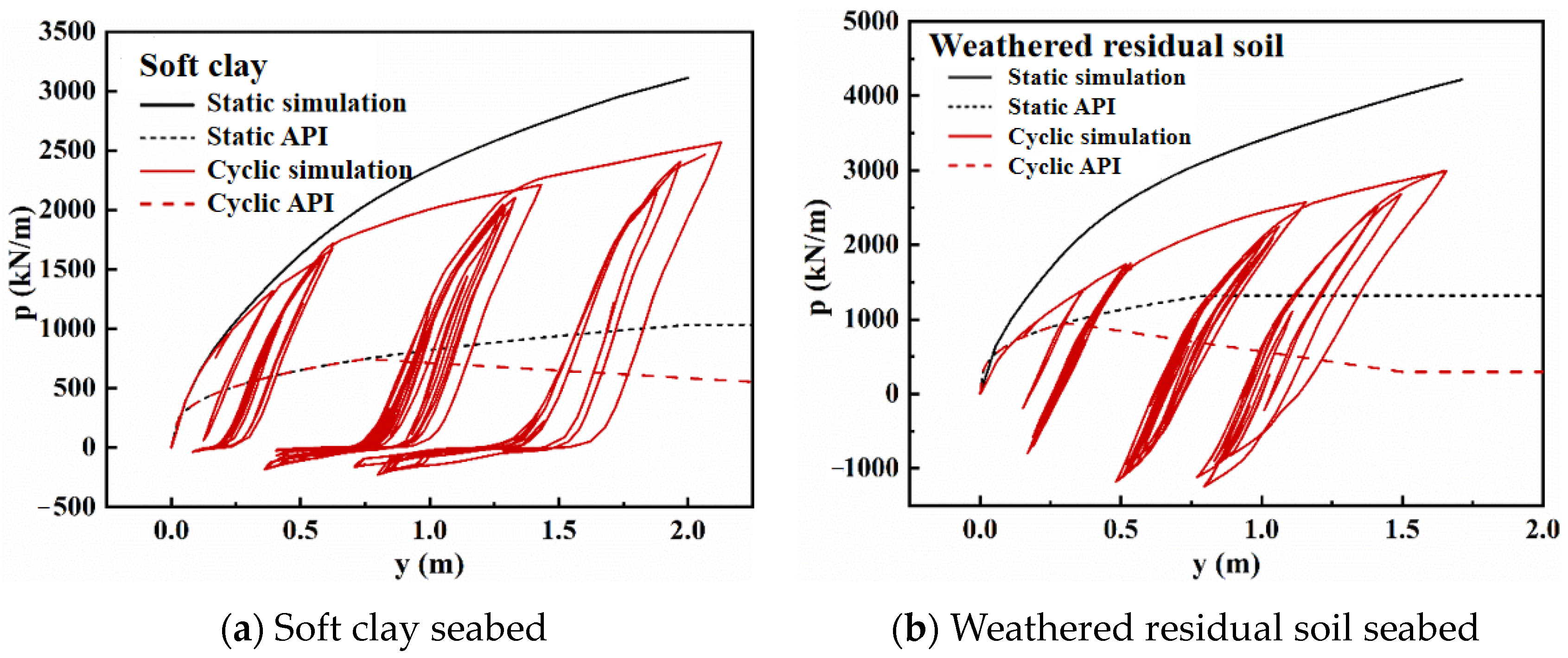
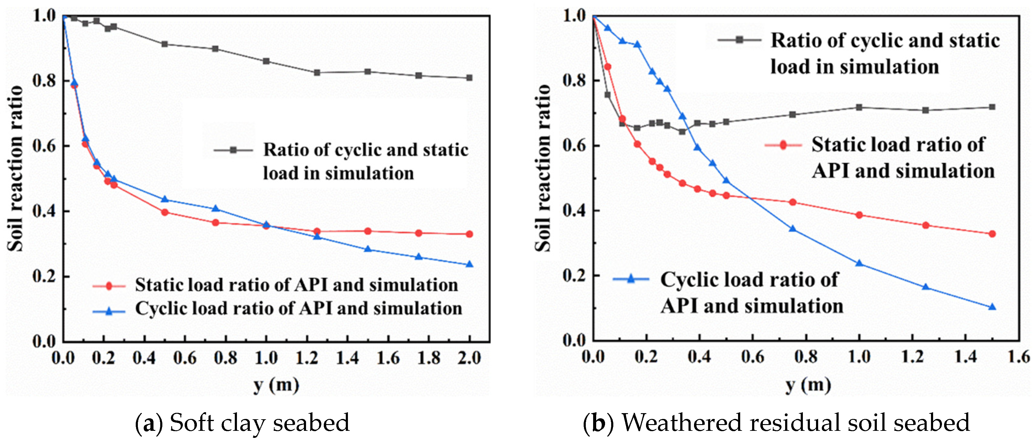
6.2.2. Comparison of p–y Curves under Different Working Conditions

Figure 16 shows the p–y curves at the −5 m burial depth under static and cyclic loads, and p–y curves calculated by API specification. The soil resistance ratios of horizontal displacement points under different working conditions are illustrated in Figure 17. The p–y curves under static loads are above that under cyclic loads in Figure 16, which indicates that the bearing capacity of the monopile foundation is weakened by the long-term cyclic loads. It is also noted from Figure 16 that the soil resistance ratios are always below 1 and decrease first and then flatten with the increase in the horizontal displacement. The soil resistance ratio under cyclic and static loads in soft clay eventually tends to 0.82, while that in weathered residual soil tends to 0.7, indicating that the monopile foundation in weathered residual soil is more susceptible to being disturbed by cyclic loads.

Figure 16. p–y curves under different working conditions and API standard at depth of −5 m.

Figure 17. Soil resistance ratio under different working conditions at depth of −5 m.

Comparing the static p–y curve calculated by numerical simulation with the static p–y curve calculated by API specification, it is found that the p–y curve calculated by API specification is below that from numerical analysis. The ratio of static soil resistance obtained by API and numerical simulation rapidly decreases when the horizontal displacement y is small (0–0.5 m). When the horizontal displacement y is greater than 0.5 m, the soil resistance ratios decrease trend slows down, which indicates that the API specification underestimates the soil resistance to a certain extent, especially in the case of large horizontal displacement. In addition, the static soil resistance ratio of API and numerical simulation in soft clay is overall greater than that in weathered residual soil, and it is obvious that the API specification is more unsuitable for weathered residual soil.

The cyclic p–y curve method recommended by API specification also significantly underestimates the soil resistance, and the underestimation degree becomes more obvious with the increase in horizontal displacement. In soft clay seabed, the changing trend of the soil resistance ratios of API cyclic p–y curves and cyclic numerical simulation is the same as that under static working conditions, the cyclic soil resistance ratios decrease rapidly from 1 to 0.4 at the initial small displacement stage, and then decrease slowly trends toward 0.2. However, the changing trend of the soil resistance ratios in weathered residual soil is different. The ratio decreases slightly with the increase in horizontal displacement, and the cyclic soil resistance ratio is also higher than the static ratio in the small displacement stage, while the cyclic soil resistance ratio is lower than the static ratio in the large displacement stage and continues to decline to 0. This is because the cyclic loads have a greater influence on the weathered residual soil.

7. Conclusions and Prospect

This paper focused on the mechanical properties of weathered residual soil and the bearing behaviors of monopile foundations in weathered residual soil. Some dynamic triaxial tests were carried out for the investigation of cyclic responses of weathered residual soil, and bearing behaviors of monopile foundation in weathered residual soil were compared with those in soft clay. The main conclusions are summarized below.

(1) The effective cohesion of the weathered residual soil is 6.57 kPa, the effective internal friction angle is 34.77°, and the stress–strain response presents strain hardening under different confining pressures.

(2) Under large cyclic loads, hysteretic curves of weathered residual soil change from a shuttle shape to an inverse S shape, and strain accumulates rapidly to the failure stage.

(3) The ultimate bearing capacities of a 5 m diameter monopile foundation in weathered residual soil and soft clay seabed are 21.3 and 14.4 MN, respectively.

(4) The bearing behaviors of monopile foundation in weathered residual soil are better than that in soft clay, and the traditional p–y design method underestimates the bearing capacity of weathered residual soil.

The main construction sites of offshore wind farms in China have gradually shifted from the soil-based seabed area to the weathered rock-based sea area, and weathered granites with different weathering degrees differ greatly. Some studies of weathered residual soil and bearing behaviors of monopiles in weathered residual soil are carried out in this paper, which is relatively limited. In the future, different weathered granites should be tested, and the bearing characteristics and design methods of pile foundations in rock-based seabed need to be studied urgently, to provide reference and solution in the construction of offshore wind power in rock-based seabeds.

References

- Alrwashdeh, S.S. Investigation of Wind Energy Production at Different Sites in Jordan Using the Site Effectiveness Method. Energy Eng. J. Assoc. Energy Eng. 2019, 116, 47–59. [Google Scholar] [CrossRef]
- Jansen, M.; Staffell, I.; Kitzing, L.; Quoilin, S.; Wiggelinkhuizen, E.; Bulder, B.; Riepin, I.; Müsgens, F. Offshore wind competitiveness in mature markets without subsidy. Nat. Energy 2020, 5, 614–622. [Google Scholar] [CrossRef]
- Yan, X.; Zhang, N.; Ma, K.; Wei, C.; Yang, S.; Pan, B. Overview of Current Situation and Trend of Offshore Wind Power Development in China. Power Gener. Technol. 2024, 45, 1–12. [Google Scholar] [CrossRef]
- Liu, D.; Liu, M.; Xu, X.; Wang, J.; Fan, C.; Li, X.; Han, J. Future prospects research on offshore wind power scale in China based on signal decomposition and extreme learning machine optimized by principal component analysis. Energy Sci. Eng. 2020, 8, 3514–3530. [Google Scholar] [CrossRef]
- Arany, L.; Bhattacharya, S.; Macdonald, J.; Hogan, S.J. Design of monopiles for offshore wind turbines in 10 steps. Soil Dyn. Earthq. Eng. 2017, 92, 126–152. [Google Scholar] [CrossRef]
- Shi, Y.; Yao, W.; Jiang, M. Dynamic analysis on monopile supported offshore wind turbine under wave and wind load. Structures 2023, 47, 520–529. [Google Scholar] [CrossRef]
- Kim, J.H.; Jeong, Y.H.; Ha, J.G.; Park, H.J. Evaluation of Soil–Foundation–Structure Interaction for Large Diameter Monopile Foundation Focusing on Lateral Cyclic Loading. J. Mar. Sci. Eng. 2023, 11, 1303. [Google Scholar] [CrossRef]
- Dai, S.; Han, B.; Huang, G.; Gu, X.; Jian, L.; Liu, S. Failure mode of monopile foundation for offshore wind turbine in soft clay under complex loads. Mar. Georesour. Geotechnol. 2022, 40, 14–25. [Google Scholar] [CrossRef]
- Alsharedah, Y.A.; Newson, T.; Naggar, M.H.; Black, J.A. Lateral Ultimate Capacity of Monopile Foundations for Offshore Wind Turbines: Effects of Monopile Geometry and Soil Stiffness Properties. Appl. Sci. 2023, 13, 12269. [Google Scholar] [CrossRef]
- Li, F.; Tian, P.; Wang, L.; Chen, M. Investigation on lateral bearing capacity of monopile under combined vertical-lateral loads and scouring condition. Mar. Georesour. Geotechnol. 2021, 39, 505–514. [Google Scholar] [CrossRef]
- Achmus, M.; Kuo, Y.S.; Abdel-Rahman, K. Behavior of monopile foundations under cyclic lateral load. Comput. Geotech. 2009, 36, 725–735. [Google Scholar] [CrossRef]
- Zhang, X.-L.; Xue, J.-Y.; Han, Y.; Chen, S.-L. Model test study on horizontal bearing behavior of pile under existing vertical load. Soil Dyn. Earthq. Eng. 2021, 147, 106820. [Google Scholar] [CrossRef]
- Dai, S.; Han, B.; Wang, B.; Luo, J.; He, B. Influence of soil scour on lateral behavior of large-diameter offshore wind-turbine monopile and corresponding scour monitoring method. Ocean Eng. 2021, 239, 109809. [Google Scholar] [CrossRef]
- Dai, S.; Yu, X.; Han, B.; He, B. Cyclic behavior of seabed building material of offshore wind farm in rock-based sea area: Submarine completely weathered granite. Ocean Eng. 2024, 296, 117024. [Google Scholar] [CrossRef]
- Han, B.; Wang, B.; Dai, S.; Hou, X.; He, B. Bearing failure mechanism of rock-socketed monopile foundation for offshore wind turbine in weathered-granite seabed. Mar. Georesour. Geotechnol. 2023, 41, 1026–1037. [Google Scholar] [CrossRef]
- Wang, Y.; Zhang, S.; Yin, S.; Liu, X.; Zhang, X. Accumulated Plastic Strain Behavior of Granite Residual Soil under Cycle Loading. Int. J. Geomech. 2020, 20, 04020205. [Google Scholar] [CrossRef]
- Zhang, X.; Zhang, X.; Xu, C.; Wu, Y. The calculation method of vertical bearing capacity of pile foundation considering cyclic weakening effect of soft clay. Comput. Geotech. 2024, 172, 106422. [Google Scholar] [CrossRef]
- Wang, M.; Wang, M.; Cheng, X.; Lu, Q.; Lu, J. A New p–y Curve for Laterally Loaded Large-Diameter Monopiles in Soft Clays. Sustainability 2022, 14, 15102. [Google Scholar] [CrossRef]
- Hamderi, M. Finite Element-Based p-y Curves in Sand. Arab. J. Sci. Eng. 2023, 48, 14183–14194. [Google Scholar] [CrossRef]
- Alver, O.; Eseller-Bayat, E.E. A dynamic p–y model for piles embedded in cohesionless soils. Bull. Earthq. Eng. 2023, 21, 3297–3320. [Google Scholar] [CrossRef]
- Lu, W.; Zhang, G. New p-y curve model considering vertical loading for piles of offshore wind turbine in sand. Ocean Eng. 2020, 203, 107228. [Google Scholar] [CrossRef]
- Oldham, D. Experiments with Lateral Loading of Single Piles in Sand; Publication of: Balkema (AA); National Academies: Washington, DC, USA, 1985. [Google Scholar]
- Byrne, B.W.; McAdam, R.A.; Burd, H.J.; Beuckelaers, W.J.A.P.; Gavin, K.G.; Houlsby, G.T.; Igoe, D.J.P.; Jardine, R.J.; Martin, C.M.; Muirwood, A.; et al. Monotonic laterally loaded pile testing in a dense marine sand at Dunkirk. Geotechnique 2020, 70, 986–998. [Google Scholar] [CrossRef]
- Achmus, M.; Abdel-Rahman, K.; Kuo, Y.S. Numerical Modelling of Large Diameter Steel Piles under Monotonic and Cyclic Horizontal Loading. In Proceedings of the Tenth International Symposium on Numerical Models in Geomechanics, Rhodes, Greece, 25–27 April 2007. [Google Scholar]
- Hearn, E. Finite Element Analysis of an Offshore Wind Turbine Generator Monopile Foundation. Master’s Thesis, Tufts University, Medford, MA, USA, 2009. [Google Scholar]
- Long, J.H.; Vanneste, G. Effects of Cyclic Lateral Loads on Piles in Sand. J. Geotech. Eng. 1994, 120, 225–244. [Google Scholar] [CrossRef]
- Verdure, L.; Garnier, J.; Levacher, D. Lateral Cyclic Loading of Single Piles in Sand. Int. J. Phys. Model. Geotech. 2003, 3, 17–28. [Google Scholar] [CrossRef]
- Peng, J.R.; Clarke, B.G.; Rouainia, M. A Device to Cyclic Lateral Loaded Model Piles. Astm Geotech. Test. J. 2006, 29, 341–347. [Google Scholar] [CrossRef]
- Byrne, B.W.; Leblanc, C.; Houlsby, G.T. Response of stiff piles to long term cyclic loading. Géotechnique 2010, 60, 79–90. [Google Scholar]
- Lesny, K.; Wiemann, J. Design Aspects of Monopiles in German Offshore Wind Farms: Proceedings of the International Symposium on Frontiers in Offshore Geotechnics; AA Balkema Publishing: Rotterdam, The Netherlands, 2005. [Google Scholar]
- Dai, H. Analysis of Steel Pipe Pile Dynamic Characteristics under Scour Conditon. Ph.D. Thesis, Southeast University, Nanjing, China, 2017. [Google Scholar]
Disclaimer/Publisher’s Note: The statements, opinions and data contained in all publications are solely those of the individual author(s) and contributor(s) and not of MDPI and/or the editor(s). MDPI and/or the editor(s) disclaim responsibility for any injury to people or property resulting from any ideas, methods, instructions or products referred to in the content. |
© 2024 by the authors. Licensee MDPI, Basel, Switzerland. This article is an open access article distributed under the terms and conditions of the Creative Commons Attribution (CC BY) license (https://creativecommons.org/licenses/by/4.0/).