Explainable Ensemble Learning Approaches for Predicting the Compression Index of Clays

Abstract

Accurate prediction of the compression index (c_c) is essential for geotechnical infrastructure design, especially in clay-rich coastal regions. Traditional methods for determining $c_c$ are often time-consuming and inconsistent due to regional variability. This study presents an explainable ensemble learning framework for predicting the $c_c$ of clays. Using a comprehensive dataset of 1080 global samples, four key geotechnical input variables—liquid limit (LL), plasticity index (PI), initial void ratio (e₀), and natural water content w—were leveraged for accurate $c_c$ prediction. Missing data were addressed with K-Nearest Neighbors (KNN) imputation, effectively filling data gaps while preserving the dataset’s distribution characteristics. Ensemble learning techniques, including Random Forest (RF), Gradient Boosting Decision Trees (GBDT), Extreme Gradient Boosting (XGBoost), and a Stacking model, were applied. Among these, the Stacking model demonstrated the highest predictive performance with a Root Mean Squared Error (RMSE) of 0.061, a Mean Absolute Error (MAE) of 0.043, and a Coefficient of Determination ($R^2$) value of 0.848 on the test set. Model interpretability was ensured through SHapley Additive exPlanations (SHAP), with $e_0$ identified as the most influential predictor. The proposed framework significantly improves both prediction accuracy and interpretability, offering a valuable tool to enhance geotechnical design efficiency in coastal and clay-rich environments.

1. Introduction

In recent years, the construction of geotechnical infrastructures along coastal areas with clay ground has gained significant popularity due to limited constructional space [1,2,3,4]. Clay ground poses unique challenges for the maintenance and design of structures, with consolidation being a crucial concern [5,6,7,8]. The compression index ($c_c$), which represents the slope of the linear segment in the e-logσ’ graph, serves as a key parameter for quantifying the compressibility of clays [9]. Generally, clays with a higher $c_c$ are more compressible and deformable under load, while those with a lower $c_c$ resist deformation better. However, conventional $c_c$ determination via oedometer testing is time-consuming and expensive, hindering efficient geotechnical assessment.

For this reason, many efforts have focused on associating fundamental geotechnical characteristics with the compression index [9,10,11]. While statistical models based on geotechnical variables like natural water content (w), liquid limit (LL), plasticity index (PI), and initial void ratio ($e_0$) have been proposed [12,13,14,15], they often lack generalizability across diverse datasets. Recent studies have shifted towards machine learning models [16,17,18], particularly ensemble learning approaches, to overcome these limitations and improve predictive accuracy. For example, Zhang et al. [19] implemented Random Forest (RF), a classic ensemble learning technique, utilizing a dataset of 311 samples with three factors: LL, PI, and $e_0$. Asteris et al. [20] developed extreme learning machine models to estimate $c_c$ using the void ratio at liquid limit, LL, and PI. Long et al. [21] employed tree-based ML algorithms to establish a correlation between $c_c$ and w, LL, PI, $e_0$, and specific gravity (G_s), drawing from 391 samples collected in Northern Iran. Lee et al. [22] gathered geotechnical data from soft ground along Korea’s southern coastline and devised a $c_c$ prediction model using linear regression analysis alongside three ensemble learning models. Díaz and Spagnoli [23] introduced a novel super-learner machine learning algorithm for $c_c$ prediction, leveraging a comprehensive dataset comprising over 1000 samples.

Nevertheless, despite the promising potential of ML models to enhance conventional methods in predicting the compression index, several challenges remain: (1) many existing models are limited by either insufficient data or a narrow geographical focus, (2) the practical application of data-driven models is often hindered by inconsistencies in real-world test data, which frequently contains missing items or values due to diverse collection methods/sites, and (3) the “black box” nature of ML models [24,25,26] makes it difficult to discern the precise relationships between geotechnical inputs and the resulting compression index.

To address these concerns, this research aims to develop an effective and interpretable machine learning framework for predicting the compression index of diverse clay samples. A comprehensive worldwide dataset is first built to mitigate regional biases. Building upon the dataset, we focus on three major contributions: (1) We employ the imputation method of K-Nearest Neighbors (KNN), therefore effectively handling the missing data. (2) We apply various ensemble learning methods, including RF, Gradient Boosting Decision Trees (GBDT), Extreme Gradient Boosting (XGBoost), and a novel use of Stacking, to model the correlations between geotechnical inputs and the compression index, conducting a comprehensive comparison to identify the most accurate and robust model. (3) We utilize the SHapley Additive exPlanations (SHAP) algorithm to interpret the predictive outcomes, providing transparent insights into feature importance and addressing the “black box” issue of ML models. These contributions result in a robust, globally applicable tool for predicting soil compression behavior, potentially enhancing the accuracy and efficiency of coastal geotechnical design and analysis across diverse geological contexts.

2. Data Overview and Analysis

A comprehensive global dataset of clay soil parameters was compiled from peer-reviewed studies, representing 1080 samples from diverse geographical regions such as Algeria, Spain, Nigeria, Iran, India, Germany, Ireland, and Bangladesh, among others [18,23,27,28,29,30,31,32,33,34] This dataset was selected to reduce regional bias and improve the generalizability of the model across a wide range of soil conditions. It encompasses four independent variables (i.e., the input features)-LL, PI (with 169 missing values), $e_0$, and w-which are used to establish a relationship with the output feature, the compression index. The selection of these four variables as input features is based on prior research into data-driven models for predicting $c_c$ [19,20,21,22,23]. These variables are critical for understanding the consolidation behavior of clays, making them ideal for building a robust and interpretable predictive model. The dataset exhibits substantial variability in both input and output variables due to differences in soil origin. Given its extensive and diverse range of data, the database is well suited for robust and reliable analysis. Key statistics of the dataset are presented in Table 1 and Figure 1.

Table 1. Statistical characteristics of the dataset.

	Maximum	Minimum	Mean	Median	SD	Range
LL (%)	199.0	17.1	45.4	44.0	14.5	181.9
PI (%)	69.0	2.0	21.3	21.5	9.0	67.0
$e_0$	7.1	0.3	0.8	0.7	0.4	6.8
w (%)	244.1	8.0	29.2	25.9	15.2	236.1
$c_c$	2.2	0.01	0.2	0.2	0.2	2.2

SD: Standard Deviation.

Figure 1. Scatter plots and distribution histograms of input and output features.

Table 1 demonstrates that the database includes clays with a broad range of plasticity, from low to very high. This is reflected in the LL values, which span 181.9%, and PI values that range from 2.0% to 69.0%. In contrast, the database also includes clays with varying degrees of compressibility, with $e_0$ ranging from 0.3 to more than 7. These statistical metrics reveal significant variability and dispersion among the variables, underscoring the comprehensive global scope of the compiled database.

Figure 1 depicts the correlation between $c_c$ and the four input features. The plots demonstrate a positive association, indicating that an increase in the input features generally corresponds to a rise in $c_c$. This correlation is particularly evident with $e_0$ and w, whereas it is less pronounced with LL and PI. These trends can be further analyzed using the Pearson correlation coefficient (r) and a correlation heatmap, as shown in Figure 2. The heatmap provides a quantitative assessment of the linear relationships between each pair of features. According to Figure 2, there is a general positive correlation between cc and all four input features, as indicated by the positive correlation values. Specifically, $c_c$ exhibits a strong positive correlation with $e_0$ (r = 0.86) and w (r = 0.88), while the correlations with PI (r = 0.1) are relatively weaker. Additionally, a strong positive correlation is observed between the two groups of input features $e_0$ and w (r = 0.91), and LL and PI (r = 0.91).

Figure 2. Correlation heatmap between different features.

3. Methodology

3.1. KNN Imputation for Missing Values

The KNN algorithm can be employed as a method for imputing missing values in the original datasets [35,36]. This technique involves selecting the k nearest neighbors of an instance with the missing data, using only the attributes with observed values. Typically, Euclidean distance is utilized to measure the dissimilarity between instances, considering only the dimensions where values are present. The missing value is then imputed by calculating the weighted average of the k nearest neighbors’ values, where the weight assigned to each neighbor is inversely proportional to its distance from the instance with the missing value.

The Euclidean distance d between instances $x_i$ and $x_j$ is:

$$d\left(x_i,x_j\right)=\sqrt{\sum _{l=1}^p{\left(x_{il}-x_{jl}\right)}^2}$$

(1)

where p is the number of dimensions and $x_{il}$ and $x_{jl}$ are the values of the l-th dimension for instances $x_i$ and $x_j$, respectively. To impute the missing value $x_i^{*}$, the weighted average is calculated as:

$$x_i^{*}={\displaystyle \frac{{\sum }_{k=1}^K\frac{x_k}{d_{ik}}}{{\sum }_{k=1}^K\frac{1}{d_{ik}}}}$$

(2)

where $x_k$ is the value from the k-th nearest neighbor, and $d_{ik}$ is the distance between the instance with the missing value and its k-th nearest neighbor.

The choice of k is crucial in KNN interpolation. A small k may make the result sensitive to nearby points and noise, leading to overfitting, while a large k can smooth the result but risk underfitting by ignoring local features. Typically, odd values like 3, 5, or 7 [37] are used to avoid ties. For this study, cross-validation determined that the optimal k was 5 based on the experimental data scale.

3.2. Ensemble Learning Algorithms

We utilized ensemble learning methods, which combine several simple models to form a more powerful and accurate prediction tool. Specifically, we used:

3.2.1. Random Forest

RF is an ensemble method that combines multiple decision trees built from bootstrapped samples. It uses Bagging (Bootstrap Aggregation) to improve accuracy and reduce variance, thus combating overfitting [38]. Each tree is trained on a random subset of the data with replacement, and feature randomness is applied when splitting nodes. For prediction, each tree votes for a class, and the class with the majority of votes is chosen as the final output. Key tuning parameters for RF [39] include the number of trees in the forest (n_estimators), the maximum depth of the tree (max_depth), and the minimum number of samples required to split an internal node (min_samples_split).

3.2.2. Gradient Boosting Decision Tree

GBDT combines decision trees with ensemble learning techniques [40]. GBDT employs boosting and classification to enhance accuracy and reduce overfitting through regularization. Decision trees are easy to interpret and handle missing features effectively, as each node depends on a single attribute. Boosting improves GBDT performance by sequentially creating a series of models that convert multiple weak classifiers into a strong, accurate predictor. Key tuning parameters for GBDT [41] include the number of trees in the estimator (max_iter), the depth of the trees (max_d), and the learning rate.

3.2.3. Extreme Gradient Boosting

XGBoost is primarily designed to enhance speed and performance through the use of gradient-boosted decision trees [42]. It generates a predictive model by leveraging a boosting ensemble of weak classification trees, employing gradient descent to optimize the loss function. XGBoost supports three key gradient boosting techniques: Gradient Boosting, Regularized Boosting, and Stochastic Boosting. It facilitates the incorporation and tuning of regularization parameters and supports parallel processing during tree construction. Critical tuning parameters for XGBoost [43] encompass the maximum number of trees ($ntree$), the minimum loss reduction required to make a further partition on a leaf node ($gamma$), and the learning rate.

3.2.4. Stacking

Stacking, also known as Stacked Generalization, is a sophisticated nonlinear modeling technique that enhances prediction accuracy by integrating multiple base estimators [44]. This approach features a two-tier structure: the first layer (level-0) consists of the base learners, while the second layer (level-1) houses the meta-learner. The outputs from level-0 are fed into level-1, a crucial mechanism in Stacking for reducing model bias. In this research, level-0 includes three base learners derived from the GBDT, XGBoost, and RF algorithms. To refine quantile regression results, ridge regression is utilized as the meta-learner at level-1.

The above ensemble learning models were implemented in Python language (version 3.7.4) by using the sklearn.ensemble library. Hyperparameters were optimized through 5-fold cross-validation combined with a grid search.

3.3. SHAP for Model Interpretability

To understand how different factors affect our predictions, we used the SHAP anlysis. This method breaks down a prediction to show the impact of each feature, helping to explain which factors are most influential. Developed by Lundberg and Lee [45], SHAP is an advanced explainable artificial intelligence (XAI) tool rooted in game theory, designed to interpret the outputs of any machine learning model. The SHAP methodology assesses each input variable’s contribution to the prediction, determining whether these contributions are positive or negative [46]. SHAP summary plots are utilized to rank the most critical features, while SHAP dependence plots analyze the impact of selected input features, thereby evaluating their influence. The SHAP approach formulates an explanatory model $g(·)$, which is expressed as follows:

$$g\left(z^{\prime }\right)={\phi }_0+\sum _{i=1}^K{\phi }_i{z}_i^{\prime }$$

(3)

where $z^{\prime }\in {\{0,1\}}^K$, and K denotes the number of independent factors; ${\phi }_i\in \mathrm{R}$ represents the SHAP value for the i-th factors; and ${\varphi }_0$ is the constant term when all independent factors are absent.

$${\phi }_i=\sum _{S\subseteq F\setminus \left\{i\right\}}{\displaystyle \frac{\left|S\right|!\left(\right|F|-|S|-1)!}{\left|F\right|!}}\left[f_{S\cup \left\{i\right\}}\left(x_{S\cup \left\{i\right\}}\right)-f_S\left(x_S\right)\right]$$

(4)

where F denotes the set of all independent factors, and S represents all subsets of F that exclude the i-th factor. Additionally, $x_S$ denotes the values of the independent factors in the subset S.

Due to the complexity of calculating SHAP values, several approximation methods have been developed, including Tree SHAP, Deep SHAP, and Kernel SHAP, the latter of which is utilized in this study [47].

3.4. Implementation Pipeline

As depicted in Figure 3, the implementation process of the proposed approach can be summarized into the following key steps:

Figure 3. Flowchart of the proposed method for $c_c$ prediction.

• Collect comprehensive global data, including LL, PI, $e_0$, and w as input features and $c_c$ as the output feature, to minimize local bias.
• Apply KNN to impute missing values in the dataset, then partition the data into training and testing sets (80% training, 20% testing).
• Train and fine-tune different ensemble learning models—RF, GBDT, XGBoost, and Stacking—to realize data-driven $c_c$ prediction.
• Assess different models using Root Mean Squared Error (RMSE), Mean Absolute Error (MAE), and Coefficient of Determination ($R^2$) to identify the best prediction model.
• Analyze and clarify the key factors influencing the performance of the best model via the interpretable machine learning algorithm SHAP.

4. Results

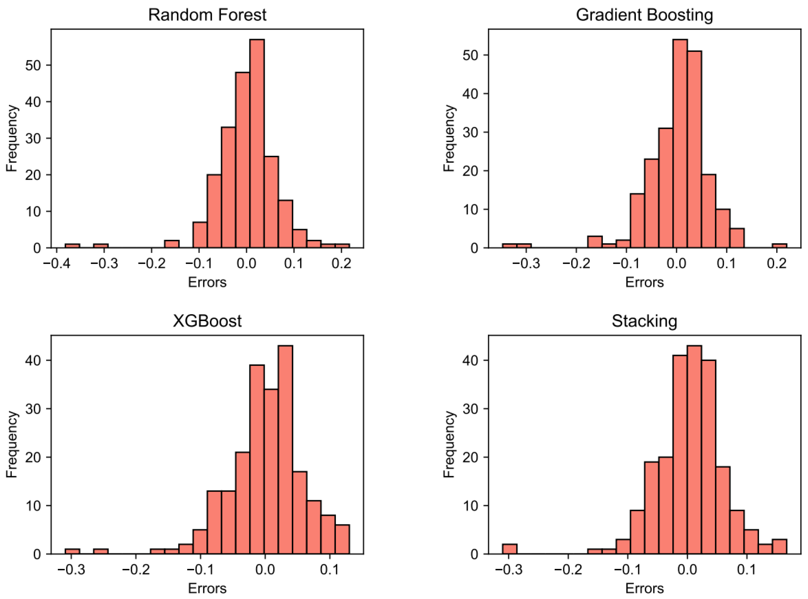
4.1. Prediction Results of ML Models

The original dataset comprises 1080 records, with 169 instances having missing values for the PI variable. Initially, the KNN method was employed to generate these missing PI values. Subsequently, the dataset was randomized to prevent the potential bias of having consecutive data from the same source within either the training or testing sets, thereby ensuring more reliable model performance and evaluation. We then divided the randomized dataset into training and testing subsets using an 80/20 split. This split ratio was selected because it is widely recognized in machine learning studies as an effective balance, providing sufficient data for training to capture underlying patterns while retaining enough data for a robust evaluation of model performance on unseen data. The four ensemble learning methods underwent hyperparameter tuning to optimize their performance, employing 5-fold cross-validation in conjunction with a grid search.

Figure 4 presents scatter plots of the actual values of $c_c$ (x-axis) versus the predicted values (y-axis) obtained from each model on the test set. As illustrated in Figure 4, the majority of data points for each ensemble learning model are clustered near the no-error line, reflecting a strong agreement between the predicted and observed values. To further assess the performance of the four ensemble learning models, a residual analysis was conducted. Residuals, defined as the differences between the predicted and actual values, are presented in Figure 5 through a histogram distribution. Analysis of this figure reveals that the residuals for all models are predominantly centered around zero and exhibit Gaussian distributions, indicating a normal distribution with minimal outliers. These observations suggest that the ensemble learning algorithms demonstrate strong generalization capabilities and do not exhibit significant prediction errors.

Figure 4. Prediction scatter plot (true values vs. predicted values) of all ML models.

Figure 5. Residuals’ histogram distribution in test sets of all ML models.

In Table 2, the RMSE, MAE, and $R^2$ values [48] for both the training and test datasets are presented for all ensemble learning models. These metrics reflect the ensemble learning models’ outstanding predictive performance and generalizability, as evidenced by the similarity in values between the training and test datasets (e.g., for the RF model: RMSE of 0.066 and 0.062, MAE of 0.044 and 0.043, and $R^2$ of 0.868 and 0.843, respectively). Overfitting occurs when a model performs significantly better on the training data than on unseen data, suggesting that it has memorized the training data rather than learning general patterns. The minimal differences between the training and test performance metrics of the models indicate their strong ability to generalize to new data and suggest that they are not prone to overfitting. Among the four ensemble models, the proposed Stacking model outperforms RF, GBDT, and XGBoost from existing research, with the test set RMSE, MAE, and $R^2$ values of 0.061, 0.043, and 0.848, respectively. Consequently, the Stacking model was selected as the optimal candidate for subsequent coupling with the SHAP algorithm for model interpretability analysis.

Table 2. Summary of performance metrics of all ML models.

Model	RMSE		MAE		${\mathit{R}}^2$
	Training	Test	Training	Test	Training	Test
RF	0.066	0.062	0.044	0.043	0.868	0.843
GBDT	0.061	0.062	0.042	0.044	0.890	0.844
XGBoost	0.062	0.063	0.042	0.043	0.884	0.839
Stacking	0.060	0.061	0.041	0.043	0.893	0.848

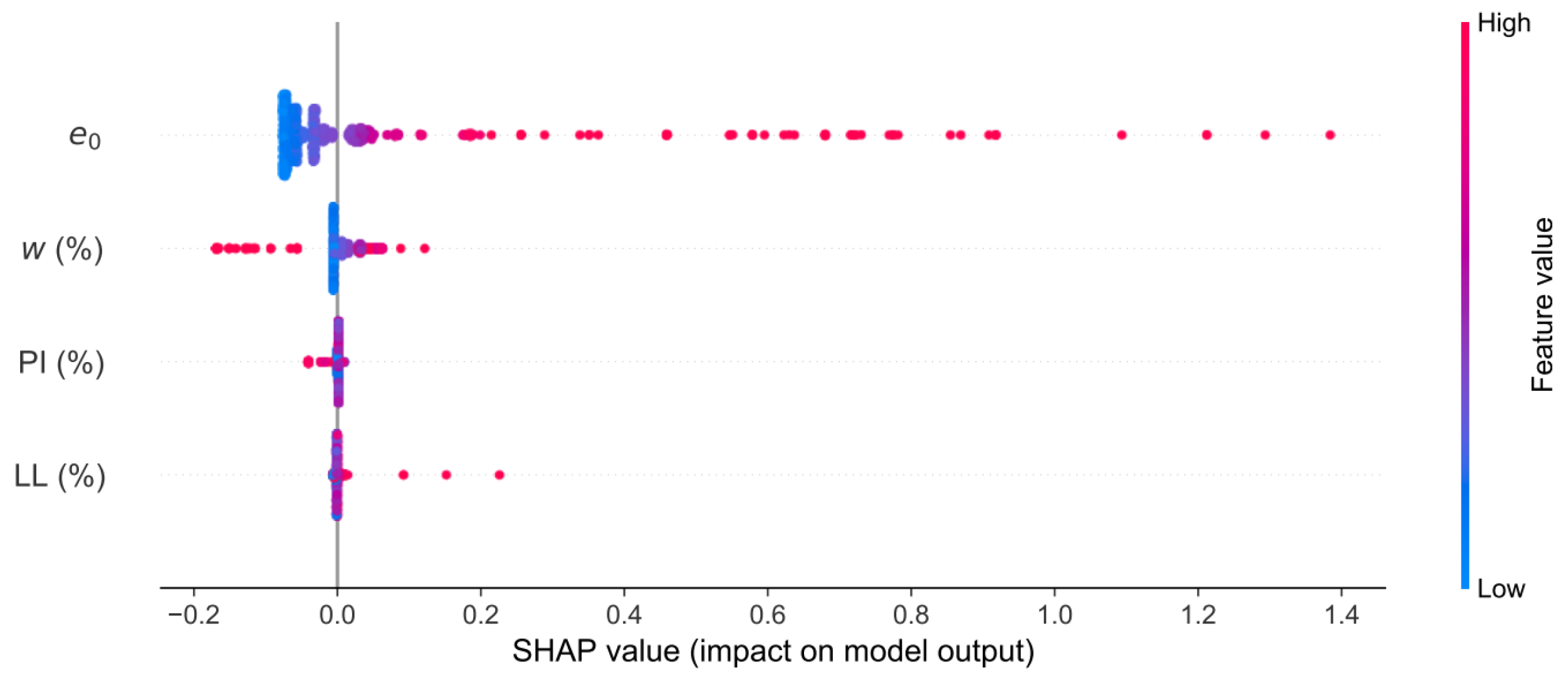
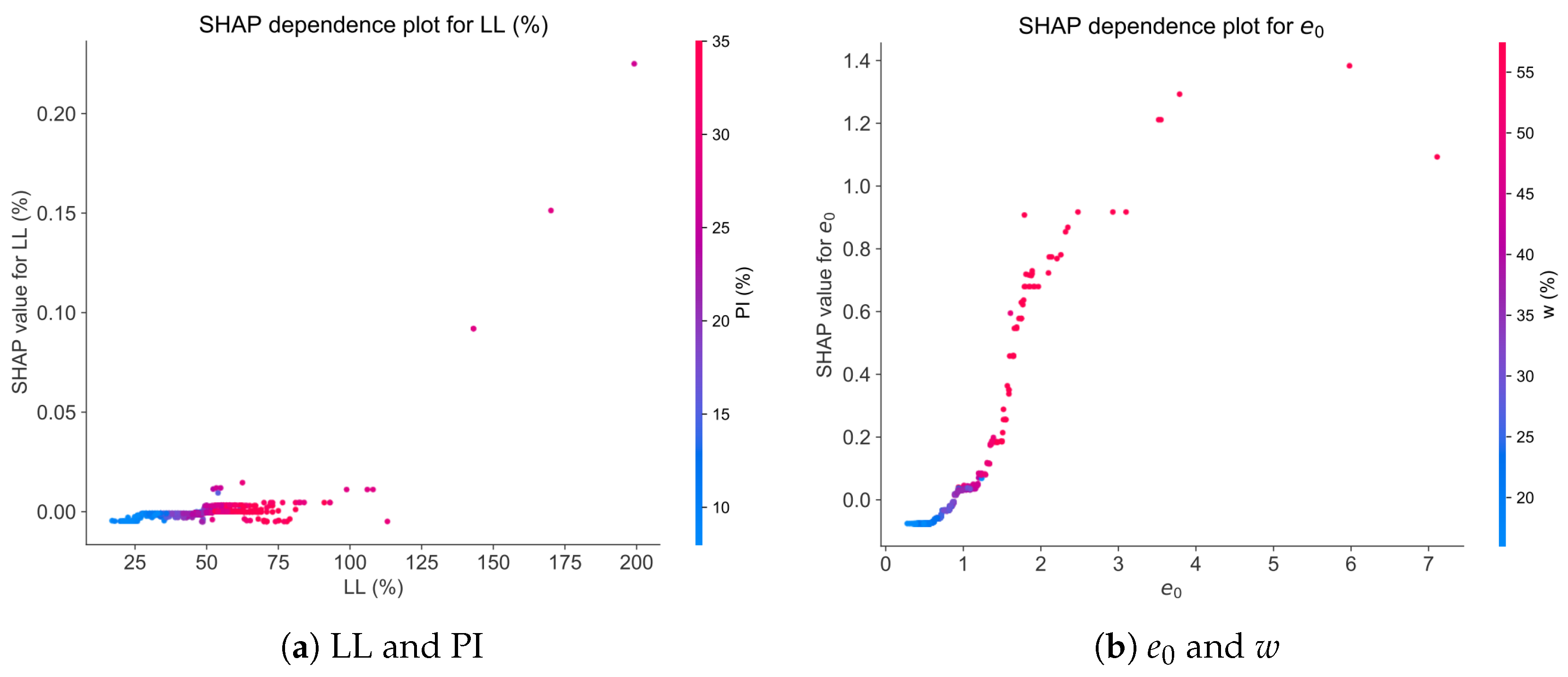
4.2. Analysis of Model Interpretability

To clarify the key factors influencing the performance of the Stacking model in predicting the compression index, we performed a factor importance analysis using SHAP. Figure 6 illustrates the importance ranking of the four independent variables. The mean absolute SHAP value plot indicates that $e_0$ exerts the greatest average impact on the model’s output, followed by w, with PI and LL having comparatively lesser influence. These results underscore the critical role of the initial void ratio and natural water content in predicting the compression index of clays, thereby emphasizing the significance of these geotechnical properties in the predictive modeling of clay behavior.

Figure 6. SHAP feature importances.

The SHAP summary plot presented in Figure 7 offers a comprehensive overview of feature importance and their effects on model predictions. In this plot, the y-axis represents the features, while the x-axis quantifies the SHAP values. Each dot signifies a Shapley value for a specific feature and instance, with color indicating feature values (red for high, blue for low). The plot reveals that $e_0$ is the most influential feature; higher $e_0$ values (red points) correlate with higher SHAP values, suggesting that increased $e_0$ levels lead to higher predicted $c_c$ values. In contrast, w exhibits a more complex impact, with both positive and negative values appearing across the SHAP value spectrum. This variability reflects its intricate relationship with the model’s output. PI and LL show relatively minor effects on predictions, aligning with the patterns observed in the previous feature importance analysis.

Figure 7. SHAP summary plot.

Finally, dependence plots for pairs of input features were created to show their joint influence on model predictions. Based on the correlation analysis in Figure 2, the four input features were grouped into two categories for detailed examination: $e_0$ and w, and LL and PI. In Figure 8, the horizontal axis shows input feature values and the vertical axis displays SHAP values. Additionally, the color bars on the right of each subplot indicate the values of the variable most dependent on the input feature shown on the horizontal axis.

Figure 8. SHAP dependence plots.

As illustrated in Figure 8a, there is a notable positive correlation between LL and PI. Specifically, when the LL values are small (with data points on the left side of the x-axis), PI values are also low (indicated by blue data points), and vice versa. This aligns with the r = 0.91 correlation coefficient reported in Figure 2. However, LL has a minimal impact on the prediction model, as indicated by the relatively flat SHAP values despite rising LL. Although PI values increase (indicated by a gradual shift in color from blue to red) as LL increases, under the joint action of the two, the SHAP value for LL shows only a slight upward trend.

Likewise, Figure 8b demonstrates a strong positive correlation between $e_0$ and w. Unlike the LL and PI groups, the SHAP value rises sharply with increasing $e_0$. However, when $e_0$ surpasses 2, the rate of SHAP value growth slows. Despite this slowdown, there is no significant color change where growth decelerates (without substantial changes in w), suggesting that $e_0$ is the primary factor affecting the SHAP value, rather than the combined effect of $e_0$ and w.

5. Discussions

The results show that interpolating missing data, constructing ensemble models, and integrating additive interpretation algorithms lead to accurate and interpretable $c_c$ predictions. Although we have compared various ensemble models and analyzed the interpretability of the optimal model, the varying degrees of missing data from different sources in practice highlight the need for effective data imputation methods. Therefore, a thorough evaluation of KNN interpolation for handling missing data in our study is necessary.

The dataset utilized in this study comprises 1080 groups of observations, with 169 instances of missing data for the input feature PI. In addition to employing the KNN interpolation method previously used, we also applied two traditional interpolation techniques—polynomial interpolation and spline interpolation—to address the missing PI data. Figure 9 illustrates the distribution patterns and characteristics of the PI raw data alongside the results after using the three interpolation methods. By analyzing the shape, peak values, symmetry, and other characteristics in histograms and density maps, we can intuitively discern the similarities and differences among different datasets.

Figure 9. Histogram and density plot of PI data after different methods of interpolation.

The figure indicates that the PI dataset interpolated using KNN closely mirrors the distribution characteristics of the original dataset. This observation is corroborated by the quantitative statistics presented in Table 3, which show that the dataset handled with KNN exhibits high consistency with the original data in key statistical measures such as mean, maximum and minimum values, median, and variance. Although polynomial and spline interpolations preserve mean and median values relatively well, they exhibit notable discrepancies in maximum and minimum values and data variance, thereby failing to replicate the original data’s distribution effectively.

Table 3. Comparison of different interpolation methods.

PI Values	Mean	Maximum	Minimum	Median	Variance
Original data with missing values	21.3	69.0	2.0	21.5	81.4
After KNN interpolation	21.6	69.0	2.0	22.0	79.6
After polynomial interpolation	21.8	100.8	−4.8	22.0	102.6
After spline interpolation	21.8	99.8	−12.2	22.0	107.1

Consequently, KNN interpolationoutperforms traditional methods by generating imputed data that accurately preserve the original dataset’s distribution, thereby providing a robust foundation for the subsequent development of high-performance machine learning models.While the K-Nearest Neighbors (KNN) imputation method was effective, it introduces some uncertainty, especially in highly variable datasets like global soil samples. Future research could explore alternative imputation methods or more complete datasets to address this issue.

6. Conclusions

This study introduces an innovative and interpretable ensemble learning framework for predicting the compression index of clays, a key parameter for geotechnical infrastructure design in clay-rich regions. This research underscores the effectiveness of integrating a comprehensive global dataset with ensemble learning models such as RF, GBDT, XGBoost, and Stacking. Among these models, the Stacking approach emerged as the most accurate, demonstrating minimal prediction errors and robust generalization capabilities.

The use of SHAP for model interpretation identified the initial void ratio as the most influential predictor of $c_c$, providing valuable insights into the geotechnical behavior of clays. This interpretable framework not only enhances prediction reliability but also offers geotechnical engineers a transparent and practical tool for real-world applications.

Moreover, this study highlights the effectiveness of the KNN imputation method for generating missing data, which preserves the original dataset’s distribution characteristics and contributes to the development of high-performance predictive models.

Although our model demonstrates strong predictive performance, future research could explore additional geotechnical parameters that affect clay compressibility. Addressing limitations such as missing data by investigating alternative imputation methods or incorporating diverse data sources could further improve model accuracy.

References

- Bugnot, A.; Mayer-Pinto, M.; Airoldi, L.; Heery, E.; Johnston, E.; Critchley, L.; Strain, E.; Morris, R.; Loke, L.; Bishop, M.; et al. Current and projected global extent of marine built structures. Nat. Sustain. 2021, 4, 33–41. [Google Scholar] [CrossRef]
- Li, J.; Chen, H.; Yuan, X.; Shan, W. Analysis of the effectiveness of the step vacuum preloading method: A case study on high clay content dredger fill in Tianjin, China. J. Mar. Sci. Eng. 2020, 8, 38. [Google Scholar] [CrossRef]
- Guo, X.; Fan, N.; Zheng, D.; Fu, C.; Wu, H.; Zhang, Y.; Song, X.; Nian, T. Predicting impact forces on pipelines from deep-sea fluidized slides: A comprehensive review of key factors. Int. J. Min. Sci. Technol. 2024, 34, 211–225. [Google Scholar] [CrossRef]
- Chen, X.; Yu, Y.; Wang, L. Assessing scour prediction models for monopiles in sand from the perspective of design robustness. Mar. Struct. 2024, 93, 103532. [Google Scholar] [CrossRef]
- Wang, J.; Dai, M.; Cai, Y.; Guo, L.; Du, Y.; Wang, C.; Li, M. Influences of initial static shear stress on the cyclic behaviour of over consolidated soft marine clay. Ocean Eng. 2021, 224, 108747. [Google Scholar] [CrossRef]
- Zheng, J.; Hu, X.; Gao, S.; Wu, L.; Yao, S.; Dai, M.; Liu, Z.; Wang, J. Undrained cyclic behavior of under-consolidated soft marine clay with different degrees of consolidation. Mar. Georesources Geotechnol. 2024, 42, 176–183. [Google Scholar] [CrossRef]
- Jiang, N.; Wang, C.; Wu, Q.; Li, S. Influence of structure and liquid limit on the secondary compressibility of soft soils. J. Mar. Sci. Eng. 2020, 8, 627. [Google Scholar] [CrossRef]
- Guo, X.; Nian, T.; Zhao, W.; Gu, Z.; Liu, C.; Liu, X.; Jia, Y. Centrifuge experiment on the penetration test for evaluating undrained strength of deep-sea surface soils. Int. J. Min. Sci. Technol. 2022, 32, 363–373. [Google Scholar] [CrossRef]
- Shimobe, S.; Spagnoli, G. A general overview on the correlation of compression index of clays with some geotechnical index properties. Geotech. Geol. Eng. 2022, 40, 311–324. [Google Scholar] [CrossRef]
- Alzabeebee, S.; Alshkane, Y.M.; Rashed, K.A. Evolutionary computing of the compression index of fine-grained soils. Arab. J. Geosci. 2021, 14, 2040. [Google Scholar] [CrossRef]
- Mawlood, Y.; Mohammed, A.; Hummadi, R.; Hasan, A.; Ibrahim, H. Modeling and statistical evaluations of unconfined compressive strength and compression index of the clay soils at various ranges of liquid limit. J. Test. Eval. 2022, 50, 551–569. [Google Scholar] [CrossRef]
- Sridharan, A.; Nagaraj, H. Compressibility behaviour of remoulded, fine-grained soils and correlation with index properties. Can. Geotech. J. 2000, 37, 712–722. [Google Scholar] [CrossRef]
- Spagnoli, G.; Shimobe, S. Statistical analysis of some correlations between compression index and Atterberg limits. Environ. Earth Sci. 2020, 79, 532. [Google Scholar] [CrossRef]
- Heo, Y.; Hwang, I.; Kang, C.; Bae, W. Correlations Between the Physical Properties and Consolidation Parameter of West Shore Clay. J. Korean GEO-Environ. Soc. 2015, 16, 33–40. [Google Scholar] [CrossRef]
- Park, H.I.; Lee, S.R. Evaluation of the compression index of soils using an artificial neural network. Comput. Geotech. 2011, 38, 472–481. [Google Scholar] [CrossRef]
- Bardhan, A.; Kardani, N.; Alzo’ubi, A.K.; Samui, P.; Gandomi, A.H.; Gokceoglu, C. A comparative analysis of hybrid computational models constructed with swarm intelligence algorithms for estimating soil compression index. Arch. Comput. Methods Eng. 2022, 29, 4735–4773. [Google Scholar] [CrossRef]
- Saisubramanian, R.; Murugaiyan, V. Prediction of compression index of marine clay using artificial neural network and multilinear regression models. J. Soft Comput. Civ. Eng. 2021, 5, 114–124. [Google Scholar]
- Benbouras, M.A.; Kettab Mitiche, R.; Zedira, H.; Petrisor, A.I.; Mezouar, N.; Debiche, F. A new approach to predict the compression index using artificial intelligence methods. Mar. Georesources Geotechnol. 2019, 37, 704–720. [Google Scholar] [CrossRef]
- Zhang, P.; Yin, Z.Y.; Jin, Y.F.; Chan, T.H.; Gao, F.P. Intelligent modelling of clay compressibility using hybrid meta-heuristic and machine learning algorithms. Geosci. Front. 2021, 12, 441–452. [Google Scholar] [CrossRef]
- Asteris, P.G.; Mamou, A.; Ferentinou, M.; Tran, T.T.; Zhou, J. Predicting clay compressibility using a novel Manta ray foraging optimization-based extreme learning machine model. Transp. Geotech. 2022, 37, 100861. [Google Scholar] [CrossRef]
- Long, T.; He, B.; Ghorbani, A.; Khatami, S.M.H. Tree-based techniques for predicting the compression index of clayey soils. J. Soft Comput. Civ. Eng. 2023, 7, 52–67. [Google Scholar]
- Lee, S.; Kang, J.; Kim, J.; Baek, W.; Yoon, H. A Study on Developing a Model for Predicting the Compression Index of the South Coast Clay of Korea Using Statistical Analysis and Machine Learning Techniques. Appl. Sci. 2024, 14, 952. [Google Scholar] [CrossRef]
- Díaz, E.; Spagnoli, G. A super-learner machine learning model for a global prediction of compression index in clays. Appl. Clay Sci. 2024, 249, 107239. [Google Scholar] [CrossRef]
- Castelvecchi, D. Can we open the black box of AI? Nat. News 2016, 538, 20. [Google Scholar] [CrossRef] [PubMed]
- Guidotti, R.; Monreale, A.; Ruggieri, S.; Turini, F.; Giannotti, F.; Pedreschi, D. A survey of methods for explaining black box models. ACM Comput. Surv. (CSUR) 2018, 51, 1–42. [Google Scholar] [CrossRef]
- Rios, A.J.; Seghier, M.E.A.B.; Plevris, V.; Dai, J. Explainable ensemble learning framework for estimating corrosion rate in suspension bridge main cables. Results Eng. 2024, 23, 102723. [Google Scholar] [CrossRef]
- Zaman, M.W.; Hossain, M.R.; Shahin, H.; Alam, A. A study on correlation between consolidation properties of soil with liquid limit, in situ water content, void ratio and plasticity index. Geotech. Sustain. Infrastruct. Dev. 2016, 5, 899–902. [Google Scholar]
- McCabe, B.A.; Sheil, B.B.; Long, M.M.; Buggy, F.J.; Farrell, E.R. Empirical correlations for the compression index of Irish soft soils. Proc. Inst. Civ.-Eng. Eng. 2014, 167, 510–517. [Google Scholar] [CrossRef]
- Saha, A.; Nath, A.; Dey, A.K. Multivariate geophysical index-based prediction of the compression index of fine-grained soil through nonlinear regression. J. Appl. Geophys. 2022, 204, 104706. [Google Scholar] [CrossRef]
- Widodo, S.; Ibrahim, A. Estimation of primary compression index (Cc) using physical properties of Pontianak soft clay. Int. J. Eng. Res. Appl. 2012, 2, 2231–2235. [Google Scholar]
- Kalantary, F.; Kordnaeij, A. Prediction of compression index using artificial neural network. Sci. Res. Essays 2012, 7, 2835–2848. [Google Scholar] [CrossRef]
- Alhaji, M.M.; Alhassan, M.; Tsado, T.Y.; Mohammed, Y.A. Compression Index Prediction Models for Fine-grained Soil Deposits in Nigeria. In Proceedings of the 2nd International Engineering Conference, Charleston, SC, USA, 1–3 April 2017; Federal University of Technology: Minna, Nigeria, 2017. [Google Scholar]
- Amagu, A.; Eze, S.; Jun-Ichi, K.; Nweke, M. Geological and geotechnical evaluation of gully erosion at Nguzu Edda, Afikpo Sub-basin, southeastern Nigeria. J. Environ. Earth Sci. 2018, 8, 148–158. [Google Scholar]
- Amagu, C.A.; Enya, B.O.; Kodama, J.i.; Sharifzadeh, M. Impacts of Addition of Palm Kernel Shells Content on Mechanical Properties of Compacted Shale Used as an Alternative Landfill Liners. Adv. Civ. Eng. 2022, 2022, 9772816. [Google Scholar] [CrossRef]
- Murti, D.M.P.; Pujianto, U.; Wibawa, A.P.; Akbar, M.I. K-nearest neighbor (k-NN) based missing data imputation. In Proceedings of the 2019 5th International Conference on Science in Information Technology (ICSITech), Yogyakarta, Indonesia, 23–24 October 2019; IEEE: Piscataway, NJ, USA, 2019; pp. 83–88. [Google Scholar]
- Jadhav, A.; Pramod, D.; Ramanathan, K. Comparison of performance of data imputation methods for numeric dataset. Appl. Artif. Intell. 2019, 33, 913–933. [Google Scholar] [CrossRef]
- Bhattacharya, G.; Ghosh, K.; Chowdhury, A.S. Test point specific k estimation for kNN classifier. In Proceedings of the 2014 22nd International Conference on Pattern Recognition, Stockholm, Sweden, 24–28 August 2014; IEEE: Piscataway, NJ, USA, 2014; pp. 1478–1483. [Google Scholar]
- Breiman, L. Random forests. Mach. Learn. 2001, 45, 5–32. [Google Scholar] [CrossRef]
- Ge, Q.; Liu, Z.q.; Sun, H.y.; Lang, D.; Shuai, F.x.; Shang, Y.q.; Zhang, Y.q. Robust design of self-starting drains using Random Forest. J. Mt. Sci. 2021, 18, 973–989. [Google Scholar] [CrossRef]
- Schapire, R.E. The boosting approach to machine learning: An overview. In Nonlinear Estimation and Classification; Springer: New York, NY, USA, 2003; pp. 149–171. [Google Scholar]
- Dong, X.; Guo, M.; Wang, S. GBDT-based multivariate structural stress data analysis for predicting the sinking speed of an open caisson foundation. Georisk Assess. Manag. Risk Eng. Syst. Geohazards 2024, 18, 333–345. [Google Scholar] [CrossRef]
- Chen, T.; He, T.; Benesty, M.; Khotilovich, V.; Tang, Y.; Cho, H.; Chen, K.; Mitchell, R.; Cano, I.; Zhou, T.; et al. Xgboost: Extreme Gradient Boosting. R Package Version 0.4-2. 2015. Available online: https://rdocumentation.org/packages/xgboost/versions/0.4-2 (accessed on 8 October 2015).
- Kavzoglu, T.; Teke, A. Advanced hyperparameter optimization for improved spatial prediction of shallow landslides using extreme gradient boosting (XGBoost). Bull. Eng. Geol. Environ. 2022, 81, 201. [Google Scholar] [CrossRef]
- Naimi, A.I.; Balzer, L.B. Stacked generalization: An introduction to super learning. Eur. J. Epidemiol. 2018, 33, 459–464. [Google Scholar] [CrossRef]
- Lundberg, S.M.; Lee, S.I. A unified approach to interpreting model predictions. Adv. Neural Inf. Process. Syst. 2017, 30, 4765–4774. [Google Scholar]
- Ma, Y.; Zhao, Y.; Yu, J.; Zhou, J.; Kuang, H. An interpretable gray box model for ship fuel consumption prediction based on the SHAP framework. J. Mar. Sci. Eng. 2023, 11, 1059. [Google Scholar] [CrossRef]
- Baptista, M.L.; Goebel, K.; Henriques, E.M. Relation between prognostics predictor evaluation metrics and local interpretability SHAP values. Artif. Intell. 2022, 306, 103667. [Google Scholar] [CrossRef]
- Ben Seghier, M.E.A.; Knudsen, O.Ø.; Skilbred, A.W.B.; Höche, D. An intelligent framework for forecasting and investigating corrosion in marine conditions using time sensor data. Npj Mater. Degrad. 2023, 7, 91. [Google Scholar] [CrossRef]
Disclaimer/Publisher’s Note: The statements, opinions and data contained in all publications are solely those of the individual author(s) and contributor(s) and not of MDPI and/or the editor(s). MDPI and/or the editor(s) disclaim responsibility for any injury to people or property resulting from any ideas, methods, instructions or products referred to in the content. |
© 2024 by the authors. Licensee MDPI, Basel, Switzerland. This article is an open access article distributed under the terms and conditions of the Creative Commons Attribution (CC BY) license (https://creativecommons.org/licenses/by/4.0/).