Abstract
This paper presents a new method for finding the optimal positions for sensors used to reconstruct geophysical fields from sparse measurements. The method is composed of two stages. In the first stage, we estimate the spatial variability of the physical field by approximating its information entropy using the Conditional Pixel CNN network. In the second stage, the entropy is used to initialize the distribution of optimal sensor locations, which is then optimized using the Concrete Autoencoder architecture with the straight-through gradient estimator for the binary mask and with adversarial loss. This allows us to simultaneously minimize the number of sensors and maximize reconstruction accuracy. We apply our method to the global ocean under-surface temperature field and demonstrate its effectiveness on fields with up to a million grid cells. Additionally, we find that the information entropy field has a clear physical interpretation related to the mixing between cold and warm currents.
1. Introduction
The problem of optimal sensor placement is of great interest in many fields, such as health [1], high-dimensional systems [2], and engineering [3]. In ocean modeling, the necessity of finding the best place to install sensors is driven by the high cost of in situ measuring platforms (e.g., [4,5]) and the need to accurately reconstruct physical fields from a limited number of measurements [6].
In our study, we will use the word “sensor” in the most general sense as a means of obtaining the value of the physical field at a particular point in space. Thus, by the “optimal” placement of sensors, we mean a finite set of spatial coordinates for which the maximum reconstruction accuracy of the physical field is achieved with a minimum number of sensors.
Classical approximations for optimal sensor placement typically assume that the measurements of the physical field at the sensor locations can be related to the physical field in the entire observation area through a linear transformation. The Fisher Information Matrix is commonly used to measure the error between the true and reconstructed fields and can be calculated as the inverse covariance matrix of the reconstruction errors. Classical methods for sensor placement can be divided into three main groups based on the loss function used [7,8]. The first group of methods maximizes the determinant of the Fisher Information Matrix or, equivalently, minimizes the determinant of the covariance error matrix [9,10,11]. The second group of methods is based on minimizing the trace of the inverse Fisher Information Matrix [12,13,14]. In particular, if the assumption of diagonal error covariance is made, the loss function is reduced to the well-known Mean Squared Error (MSE) between the observed and reconstructed fields. The third group of classical methods minimizes the maximum eigenvalue of the inverse Fisher Information Matrix or equivalently minimizes the spectral norm of the error covariance matrix [12,13].
Singular Value Decomposition (SVD) and QR decomposition are commonly used for finding optimal sensors in linear methods. However, these methods face challenges when applied to high-dimensional data, as they scale cubically and quadratically with the dimensionality of the data for full and truncated SDV, respectively. This can make them computationally intensive, even with the use of massively parallel computing systems. Additionally, these linear methods may produce non-physical results due to the lack of consideration for physical constraints.
Recently, deep learning methods have been increasingly used to analyze climate data at high resolution and improve operational forecasting systems. For example, in [15], it was shown that modern deep learning models with transformer architecture could be comparably accurate to classical numerical models in short-term forecasting of the state of the atmosphere on a grid of 0.25 degrees. However, classical numerical models still outperform deep learning models when it comes to the medium- and long-term forecast of the Earth system.
The introduction of the Gumbel-softmax distribution [16] and concrete distribution [17] made it possible to use traditional gradient-based methods to optimize the parameters of discrete probability distributions. Several deep-learning models for optimal sensor placement have been proposed. These include the Concrete Autoencoder [18,19], deep probabilistic sampling [20], and feature selection networks [21]. These deep learning methods are more memory efficient and do not require the computation of expensive covariance matrices. However, optimization using the Gumbel-softmax trick can require a long exploration period to find the optimal sensor locations. In [22], Shallow Decoder Networks (SDNs) were introduced with two algorithms for optimizing sensor locations: a linear selection algorithm based on QR decomposition (Q-SDN) and a nonlinear selection algorithm based on neural network pruning (P-SDN). Pruning-based sensor search is similar to the annealing of the temperature parameter in the Concrete Autoencoder by [18], but it also enables an automatic search for the optimal number of sensors. In contrast, in [18], the number of sensors was fixed from the start.
Using a high-resolution World Ocean model exclusively for solving the sensor placement problem through a direct combinatorial search is impractical due to its high computational intensity and long duration of a single experiment. A potential solution is to use a hybrid approach that combines statistical processing of retrospective hydrodynamic modeling data using neural network models to capture nonlinear dependencies, followed by the assessment of the sensor locations using an ocean general circulation model. This approach allows for physically justified optimal sensor coordinates to be obtained within an acceptable timeframe. Furthermore, it scales linearly with the size of the computational domain and does not require computing the covariance matrix of the numerical solution. This makes it well-suited for applications such as global ocean circulation models with a resolution of 0.25 or 0.1 degrees, where the covariance matrix as a vector can have dimensions of to .
The aim of this research is to explore the feasibility of using modern neural network methods to determine the optimal locations for temperature sensors in the World Ocean at 0.25-degree resolution. We propose a Concrete Autoencoder architecture and training procedure that improve the methodology proposed in [23], where it was tested for a relatively small grid of size . The method uses an adversarial loss and a differentiable feature selection by using straight-through gradient estimation. Our approach is applicable to high-resolution grids and utilizes entropy initialization to accelerate the convergence of the sensor sparsification algorithm. It includes a reconstruction operator, which uses the measurements to try to reconstruct the physical field at the full computational grid. The sensor placement and the reconstruction operator are jointly optimized using a binary mask as a parameter.
This paper is organized into five sections. The introduction is provided in Section 1. In Section 2, we describe a method for approximating the information entropy field and present a Concrete Autoencoder architecture for optimizing sensor placement. We also provide a method for analyzing sensor-perturbing sensitivity using the autoencoder and approximate the region of influence of an observation using mutual information. In Section 3, we describe the training and the test datasets, baselines, and evaluation metrics. In Section 4, we present numerical results for a high-resolution grid and discuss the geophysical interpretation of the obtained information entropy field and sensitivity. Finally, we provide our main conclusions in Section 5.
2. Materials and Methods
The developed methods for optimizing sensor placement and determining the area of influence of individual sensors can be divided into four components, as illustrated in Figure 1. The orange blocks represent the information entropy approximation (Section 2.1). The blue blocks refer to the optimization of sensor placement using the Concrete Autoencoder (Section 2.2). The yellow block indicates the sensitivity analysis method, which utilizes a trained Concrete Autoencoder (Section 2.3). Lastly, the purple block describes the methods of assessing the sensitivity of a sensor through mutual information (Section 2.4). The input data, which are indicated by the green blocks for these procedures, are specified further in Section 3.1.
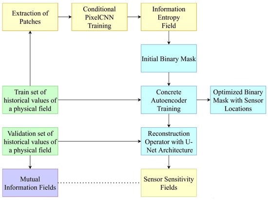
Figure 1.
Dependence scheme of the developed methods in the general process of optimizing the sensor placement and finding its area of influence. The orange blocks describe the information entropy approximation. The blue blocks correspond to the optimization of sensor placement using a Concrete Autoencoder. The yellow block corresponds to the sensitivity analysis method, which utilizes a trained Concrete Autoencoder. The purple block describes the methods of assessing the sensitivity of a sensor with the help of mutual information. The green blocks indicate the input data.
2.1. Approximation of the Information Entropy Field
To apply optimization algorithms efficiently in a high-dimensional space of sensor locations, it is necessary to introduce an informative prior distribution. One approach is to place sensors at points where the physical field has high variability. This can be achieved by defining a non-negative scalar field that reflects the historical variability of the physical field and using it to define the prior distribution as:
where is a temperature parameter that controls the concentration of sensors near the maximum of the variability field . At the first stage of our method, we estimate the variability of the physical field as a function of spatial coordinates r by approximating its information entropy. To handle non-normally distributed variables, we use deep neural networks to approximate the probability density. This approach can be applied to spatially correlated non-Gaussian random variables by using the Conditional Pixel Convolutional Neural Network (PixelCNN) [24,25] to approximate the joint probability density of patches taken from a dataset of historical values of physical fields.
Suppose that we have a set of N patches with sizes cropped from the K-dimensional domain of interest , each of which is labeled with spatial coordinates of the patch center
Our goal is to approximate the probability density of physical fields as a function of spatial coordinates r. A single patch can be represented as a vector of dimension , and the probability density can be expanded as the product of probabilities of individual pixels, each of which is conditioned on all previous pixels:
where stands for the i-th pixel of image with respect to the chosen ordering.
Conditional PixelCNN is designed to generate images by predicting the values of individual pixels in the image, given the values of previous pixels. This is achieved by using a convolutional neural network (CNN) with a special architecture known as a PixelCNN, which is able to capture the dependencies between pixels in an image and generate samples that are highly realistic and detailed. PixelCNN uses masked convolutions to ensure that a generated pixel depends only on the previous ones. The use of conditional information, such as class labels or other features, allows the model to generate images that are conditioned to specific characteristics, such as the presence of specific objects or styles. This makes it a powerful tool for tasks such as image generation, inpainting, and density estimation. In this study, we employ a Conditional PixelCNN configuration with 15 convolutional layers, each with 64 hidden channels, resulting in a network with 6.0 million parameters.
To compute the information entropy from the probability density of a system, we first need to approximate a Probability Distribution Function (PDF) that describes the density (see Algorithm 1). Once we have approximated the PDF, we can compute the information entropy using the following formula:
where I is the information entropy, is the conditional PDF of the system, and s is a variable that represents the possible states or outcomes of the system.
To reduce the dependence of the information entropy field from the random weight initialization of the Conditional PixelCNN, we train an ensemble of several models, . Final information entropy is obtained by averaging over the ensemble
where represents the information entropy of the individual ensemble members and is obtained by the following Monte Carlo approximation
| Algorithm 1 Information Entropy Approximation. |
|
2.2. Concrete Autoencoder for Sensor Placement Optimization
In the second stage, the entropy of the physical field is used to initialize the distribution of sensor locations; since the density of the initial locations is proportional to the information entropy. This configuration is further optimized by the Concrete Autoencoder architecture to simultaneously minimize the number of sensors and maximize the reconstruction accuracy. At the initial warm-up stage of the optimization, the maximum possible reconstruction accuracy is achieved. As the optimization continues, the number of sensors gradually reduces due to an increase in the loss term associated with the number of sensors. This process allows for a substantial reduction in the number of sensors without a significant decrease in the accuracy of the physical field reconstruction.
Our Concrete Autoencoder architecture consists of a trainable binary mask and a reconstructing image-to-image neural network with a U-Net architecture [26] and bilinear upsampling. The U-Net configuration has four down-sampling and four up-sampling blocks, each of which reduces the resolution of the feature tensor by a factor of two and doubles the number of feature channels. This network has a total of 31.0 million parameters. The detailed network architecture is presented in Figure 2.
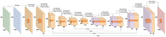
Figure 2.
Detailed architecture of the Concrete Autoencoder. The green box indicates the original input physical field. The blue box corresponds to the binary mask that determines sensor locations. The orange blocks present down-sampled features obtained from the measurements at the sensor locations. The purple blocks indicate the up-sampled feature tensors. The red block represents the reconstructed physical field. For each convolution block, the shape of the convolution kernel is presented in the format (kernel height, kernel width, number of input channels, number of output channels).
The U-Net takes, as input, a physical field multiplied by the binary mask and predicts the reconstructed field in the full computational domain. Our binary mask representing sensor locations is parametrized by the scalar field of parameter w via a step function
To determine the optimal number of sensors, we optimize the parameters of the binary mask using a straight-through gradient estimator proposed in [27] with gradient clipping. In the backward pass, we replace the ill-defined gradients of the step function with the gradients of the identity function. The straight-through gradient estimator allows us to use a single matrix w of parameters for different numbers of sensors.
The loss function of the Concrete Autoencoder has three main terms
where dynamically changes during training. In the first warm-up stage, , this is performed to initially achieve good reconstruction quality. Next, at the sparsification stage, is increased by at every epoch. This allows the Concrete Autoencoder to minimize the number of sensors without a significant increase in the reconstruction error. A similar procedure was proposed in the original version of the Concrete Autoencoder [18] where the annealing procedure was applied to the temperature parameter of the Gumbel-softmax distribution.
Consider a random batch sampled from . Following Pix2Pix framework [28], the loss function requires that the Concrete Autoencoder produces physical fields that are indistinguishable by the PatchGAN discriminator from the real fields
In addition to the requirement for the realism of the generated physical fields, we require an element-by-element correspondence of the reconstructed physical fields with the ground truth ones. The -norm is used to measure pixel-wise error
The sparsification of sensors is achieved by adding the average value of the binary mask to the loss function
We require the discriminator to distinguish the physical fields produced by the Concrete Autoencoder from the real ones, thus defining its loss as
The full training procedure for the Concrete Autoencoder is outlined in Algorithm 2.
| Algorithm 2 Concrete Autoencoder Training. |
|
2.3. Sensitivity Analysis for Sensor Measurements
After the Concrete Autoencoder is trained, we can investigate the area of influence of a sensor by perturbing the sensor measurements and examining the resulting changes in the reconstructed field. This can help us understand how changes in a sensor’s measurements affect the overall accuracy of the reconstructed physical field.
The sensitivity field can be computed by perturbing a sensor measurement with Gaussian noise and recording the resulting reconstructed fields. Since a single forward pass of the Concrete Autoencoder network takes less than a second, and an ensemble of the perturbed reconstructed fields can be constructed in a few minutes. The sensitivity field can then be derived as a field of standard deviations, as outlined in Algorithm 3.
| Algorithm 3 Sensitivity field computation from a trained Concrete Autoencoder. |
|
2.4. Mutual Information Field
As an independent method for evaluating the sensitivity of the reconstruction of measurements and the influence of measurements at a specific point on the entire computational domain, we also calculated the field of mutual information [29,30]. The calculation was performed for a specific measurement coordinate pairwise with all other points. A detailed description of the procedure is provided in Algorithm 4.
| Algorithm 4 Mutual Information Approximation. |
|
This algorithm estimates the mutual information for a given dataset of physical field realizations. The input is a training dataset containing field values at each point r at a series of time moments. The dataset is first normalized by subtracting the multiyear monthly average value for each point r and dividing by the standard deviation. The normalized values are then converted to discrete bins.
Next, the mutual information field is calculated for each point p using the joint probability mass function of the discrete bin values for that point and all other points r. The mutual information is computed as the sum of the joint probabilities multiplied by the log of the ratio of the joint probability to the product of the marginal probabilities.
3. Numerical Experiments
The training dataset for this study contains daily temperature fields for 9, 135, and 1250 m depth levels taken from the INMIO global ocean circulation model hindcast. The data covers a period from 2 January 2004 to 31 December 2020, and the calculation of the training dataset for 17 model years took approximately 340 h using 239 processor cores, including 176 cores for the ocean, 60 cores for ice, and 3 cores for the coupler, atmospheric forcing, and rivers runoff. The number of processors was chosen to ensure that the time for calculating the integration steps for the ice and ocean models was approximately equal, leading to more efficient use of computing resources when scaling the model to larger grids. This issue is discussed in further detail in [31].
The test set for this study was chosen to be the INMIO reanalysis from 1 January 2020 to 31 December 2020. During the reanalysis experiment, ocean and ice state observations, including ARGO temperature and salinity profiles [4,32], AVISO sea surface height [33], and EUMETSAT/OSISAF ice concentration [34], in the northern and southern hemispheres were assimilated using the Ensemble Optimal Interpolation (EnOI) scheme with an ensemble of 209 elements. The calculation of one model year for the test dataset took approximately 50 h using 208 cores, including 120 cores for the ocean, 72 cores for ice, 10 cores for EnOI, and 16 cores for the coupler, atmospheric forcing, and rivers runoff.
We trained the Concrete Autoencoder with Adam optimizer and computed the daily climate based on the training set. After training, we computed the reconstruction error on the test set and compared all methods using bias and RMSE metrics. The neural networks were trained using the compute nodes with Nvidia Tesla V100 GPUs. The information entropy field was computed by averaging across the ensemble of Conditional PixelCNN networks. For every depth level out of the three considered, an ensemble of three Conditional PixelCNN networks was trained, which for a single ensemble element took 60 h on a single V100 for patch size . The training of a single Concrete Autoencoder takes about 160 h on a single V100 for a computational grid of size . Therefore, in total, neural network training took about 340 GPU-hours per field for every level.
Theoretically, the computational time of our method scales linearly with the number of computational cells in the ocean model. However, this depends on the amount of data used for training and the available computational resources. At present, for global operational ocean forecast systems, the maximum resolution is of a degree [35], which is limited by the number of CPU cores and RAM in the computing cluster being utilized. In our study concerning data with degree resolution (which is about 28 km at the equator), we utilized approximately 300 CPU cores for generating the data and 8 GPUs with 32 GB of GPU memory for neural network training. With a larger compute cluster featuring 1000–2000 CPU cores and 8–10 GPUs with 80 GB of GPU memory, it is possible to extend the method to a resolution of 1/10 degree or 11 km.
3.1. Datasets Description
INMIO Ocean general circulation model. The system of equations of three-dimensional ocean dynamics and thermodynamics in the Boussinesq and hydrostatic approximations is solved by the finite volume method [36] on the type B grid [37,38,39]. The ocean model INMIO [40] and the sea ice model CICE [41] operate on the same global tripolar grid with a nominal resolution of . The vertical axis of the ocean model uses z-coordinates on 49 levels with a spacing from 6 m in the upper layer to 250 m at the depth. The barotropic dynamics are described with the help of a two-dimensional system of shallow water equations by the scheme [42]. The horizontal turbulent mixing of heat and salt is parameterized with a background (time-independent) diffusion coefficient equal to the nominal value at the equator and scaled toward the poles proportionally to the square root of the grid cell area. To ensure numerical stability in the equations of momentum transfer, the biharmonic filter is applied with a background coefficient scaled proportionally to the cell area to the power 3/2 and with the local addition by Smagorinsky scheme in formulation [43] for maintaining sharp fronts. Vertical mixing is parameterized by the Munk–Anderson scheme [44], with convective adjustment performed in the case of an unstable vertical density profile. At the ocean–atmosphere interface, the nonlinear kinematic-free surface condition is imposed with heat, water, and momentum fluxes calculated by the CORE bulk formulae [45]. Except for vertical turbulent mixing, all the processes were described using time-explicit numerical methods, which allow simple and effective parallel scaling. The time steps of the main cycle for solving model equations are equal for the ocean and the ice. The ocean model, within the restrictions of its resolution, implements the eddy-permitting mode by not using the laplacian viscosity in the momentum equations.
The sea ice model CICE v. 5.1. For this experiment, an elastic-viscous-plastic rheology model was applied to parameterize the ice dynamics, and zero-layer approximation was used for thermodynamics calculations. To explicitly resolve elastic waves, a subcycle with small time steps was set. The simulation mode includes the processing of five categories of ice thickness and one category of snow thickness using an upwind transport scheme and a description of melt ponds.
ERA5 atmospheric forcing. We used the ERA5 reanalysis [46] for the period 2004–2020 as the external forcing to determine the water and momentum fluxes on the ocean–atmosphere and ice–atmosphere interfaces. Wind speed at 10 m above sea level and temperature and dew point temperature at 2 m were transmitted to the ice–ocean system every 3 h. In addition, the accumulated fluxes of incident solar and long-wave radiation and precipitation (snow and rain) were also read with the same period.
EnOI. A detailed description of the EnOI method is presented in the work [47]. For our calculation, we used the original parallel realization of the EnOI method for data assimilation in the INMIO model [48].
The basic equations of the EnOI method are as follows [49]:
where K is defined as
(background) and (analysis) are vectors of size n representing the model solution before and after data assimilation, respectively; n is the number of model grid points weighted by the number of model variables to be corrected (temperature, salinity, sea level, etc.); is the vector of observations of size m; m is the total number of observation points where various data were obtained; is the gain matrix; is the covariance matrix of observation errors, it is assumed that the matrix is the identity matrix multiplied by a scalar parameter r; is the matrix, representing the projection operator of model values into the observational data space; is the covariance matrix of model errors.
The EnOI method belongs to a group of assimilation methods that rely on some approximation of matrix B based on an ensemble of model solution vectors. This approximation allows for the estimation of the covariance matrix of model errors. In practice, the ensemble is used to approximate matrix of size . The inverse is then computed using SVD, which can be a limiting factor in the assimilation of a large number of observations.
3.2. Baseline
Climate. The simplest baseline in ocean modeling, reconstruction, and forecasting is climate interpolated in time to the correct date. We calculated our climate values on the training set for every day of a year, according to the formula
where is the value of a physical field with coordinates at day number in year y from the training set, is the number of years with day d in the training set.
3.3. Evaluation Metrics
In this study, we use evaluation metrics based on the GODAE OceanView Class 4 forecast verification framework [50]. The bias metric measures the correspondence between the mean forecast and the mean observation. To calculate the spatial and temporal distributions of the bias, we average over time at each spatial location using Equation (7) and average over the spatial coordinates at each time point in the test set using Equation (8), respectively.
where is the reconstructed values of a physical field at a point with coordinates and at time moment , is the original reanalysis values of a physical field in the same point.
where is the total number of computational cells for the field considered.
4. Results
In this section, we demonstrate the developed methods. In Section 4.1, information entropy fields are presented. Section 4.2 discusses the balance between the number of sensors and the reconstruction accuracy during the training of the Concrete Autoencoder. Section 4.3 presents the reconstructed fields by the Concrete Autoencoder, climate, and baseline methods, which utilize the Nearest Neighbor interpolation. In Section 4.4, the reconstruction accuracy of the models is investigated in terms of RMSE and bias on the test dataset and compared to the baselines. The sensitivity of the reconstructed fields to individual measurements is studied in Section 4.5 and compared to the mutual information fields.
In the course of data-driven optimal sensor placement studies [3,8,9,51], it is customary to analyze global sea surface temperature (SST) data as a validation case. Therefore, we consider the optimal sensor locations and reconstruction of the temperature field from the top ocean layer at 9 m depth. However, the information entropy field is shown at a depth of 135 m because at the stage of analysis, it became clear that this level is of greater interest and clearly corresponds to the local hydrophysical features. The field of information entropy at a depth of 9 m can be viewed in Appendix A.
4.1. Information Entropy
Information entropy was calculated for layers at depths of 9 (Figure A1), 135 (Figure 3), and 1250 m (Figure A2). The layer at a depth of 135 m (Figure 3) is of particular interest from a hydro-physical perspective, as it is at a depth where the atmosphere has little direct influence, and ocean dynamics are active. This makes it a suitable depth for comparing the information entropy field to the behavior of real ocean currents.
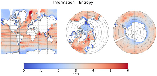
Figure 3.
Information entropy field of the temperature at 135 m depth.
In Figure 3, low-information entropy can be observed in regions where the ocean temperature does not change significantly throughout most of the year. This indicates that we had a greater degree of a priori information about the undersurface temperature in these regions. We found that IE reaches its maximum values in regions where warm and cold waters mix, and the boundary between them is likely to fluctuate, such as to the northwest of Spitsbergen, to the east of Argentina, and in the Arabian and Japanese seas. These areas are characterized by the mixing of cold and warm currents, which can lead to significant uncertainty in ocean conditions.
To the northwest of Spitsbergen, the boundary between the warm West Spitsbergen and cold East Greenland currents results in a high level of uncertainty, likely due to the “atlantification” of the Arctic Ocean, which refers to the strengthening of the influence of waters of Atlantic origin on the hydrophysical regime of the Arctic Ocean (see [52]). To the east of Argentina, the confluence of the cold Falkland Current and the warm Brazil Current also exhibits high IE values. The high levels of information entropy observed in the Arabian Sea may be attributed to two factors. First, the direction of ocean currents in the upper 200 m of the ocean changes seasonally due to the prevailing easterly trade winds in the northern hemisphere winter and strong southwest monsoon in the summer. Secondly, there has been a trend of rapid warming of the upper 700 m of the ocean in the tropical Indian Ocean over the past 70 years [53]. These factors likely contribute to the high levels of uncertainty in this region. In the Sea of Japan, the intra-annual variation of two currents, the Tsushima warm current [54] and the Liman current, carrying colder water from the Sea of Okhotsk, is likely the cause of the high IE observed.
4.2. Training Dynamics of the Concrete Autoencoder at the Sensor Sparsification Stage
After computing the information entropy field , we use it to initialize the binary mask with approximately 60,000 sensors, which are independently sampled from the prior distribution
with the temperature parameter .
During the warm-up stage, the Concrete Autoencoder is trained with a fixed binary mask and for 50 epochs to improve reconstruction quality. To encourage sparsification of the binary mask defining the positions of sensors, the weight of the corresponding term in the loss function is gradually increased. In the sparsification stage, is initially set to 4 and increased by 1.0 every 5 epochs.
Figure 4a shows the dynamics of the RMSE between reconstructed and ground truth temperature fields during the training. The initial RMSE is low due to the warm-up stage, and it gradually increases as the number of sensors decreases. The reconstruction error remains relatively low as the number of sensors exponentially decreases from 60,000 to around 1500 over the first 400 epochs, as shown in Figure 4b. Spikes in the RMSE plot can be observed when the weight of is increased. After the number of sensors drops below 800, the reconstruction error starts to grow significantly. The dynamics of RMSE in comparison with the number of sensors is illustrated in Figure 4c.
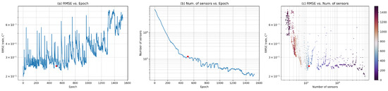
Figure 4.
The training dynamics of the Concrete Autoencoder at the sensor sparsification stage. (a) RMSE as a function of epoch, (b) number of sensors as a function of epoch, and (c) RMSE as a function of the number of sensors, with the epoch indicated by the color bar. The red dots in (a–c) denotes the Concrete Autoencoder checkpoint used in further analysis.
To analyze the reconstruction quality of the Concrete Autoencoder, we choose the checkpoint at epoch 508, when the number of sensors is 1236 and RMSE stays relatively low. The corresponding sensor locations are shown in Figure 5. For comparison, the reconstruction quality was also analyzed using the Nearest Neighbor method applied to a regularly spaced grid of sensors, as depicted in Figure 6.
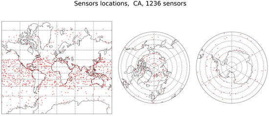
Figure 5.
Locations of 1236 sensors from the Concrete Autoencoder (CA) checkpoint at epoch 508.
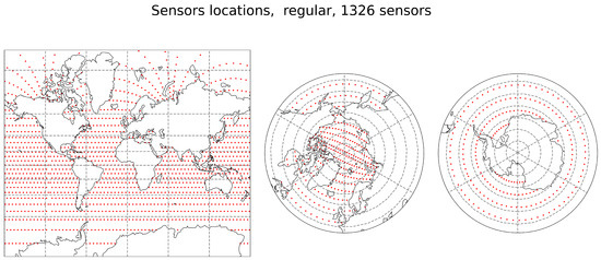
Figure 6.
Locations of the 1326 sensors regularly placed.
4.3. Reconstructed Fields
In this subsection, we present the temperature fields reconstructed using several methods. Figure 7 shows the original temperature field for 29 July 2020. Figure 8 shows the field reconstructed with the Concrete Autoencoder using 1236 sensors. Figure 9 shows the field reconstructed using climate data. Figure 10 shows the field reconstructed using the Nearest Neighbor method with 1326 regularly placed sensors shown in Figure 6. The Concrete Autoencoder, in terms of detail, resembles an improved climate. This means that the fields are as blurry as when predicting with the help of climate, but thanks to the sensors, individual regions are, on average closer to reality, as can be seen in the Arctic north of Spitsbergen and north of the Laptev Sea. In the case of the Nearest Neighbor method, a mosaic structure is observed in the reconstructed field, and as the number of sensors increases in Figure A3, the reconstructed field approaches the original field, as shown in Figure A5.

Figure 7.
Original temperature field from the test set at 9 m depth, 29 July 2020.

Figure 8.
Reconstructed field by the Concrete Autoencoder (CA) from 1236 sensors.
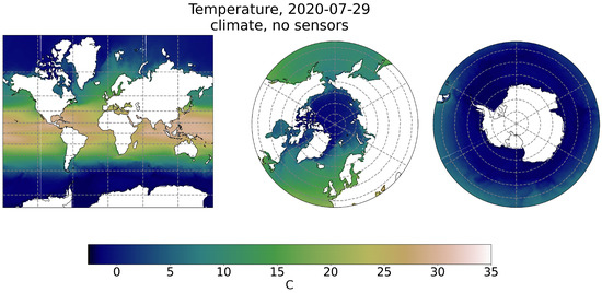
Figure 9.
Reconstructed field from the climate without measurements.
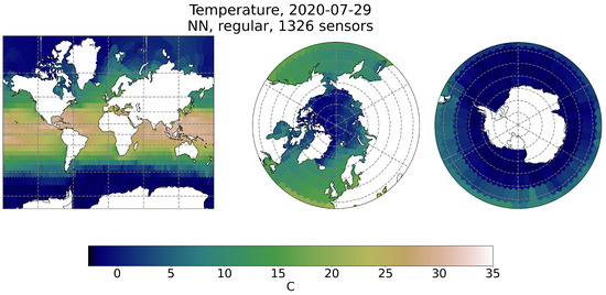
Figure 10.
Reconstructed field using the Nearest Neighbor (NN) method from 1326 measurements with regular placement.
4.4. Reconstruction Accuracy
The accuracy metrics calculated using Equations (7) and (9) are shown in Figure 11, Figure 12, Figure 13 and Figure 14. The median values were calculated from the time series of and using Equations (8) and (10), and the corresponding historical time series are shown in Figure 15. The total reconstruction accuracy for all methods is shown in Table 1. The spatial distribution of the temperature field reconstruction accuracy by the Nearest Neighbor method is shown in Appendix A for 1326 regularly placed sensors in Figure A8 and Figure A9 and 8671 regularly placed sensors in Figure A10 and Figure A11, as well as for 1236 sensors placed by the Concrete Autoencoder in Figure A6 and Figure A7.
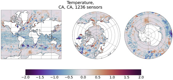
Figure 11.
Spatial distribution of reconstruction bias by the Concrete Autoencoder (CA) from 1236 measurements.
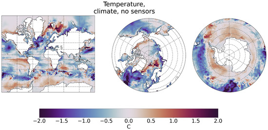
Figure 12.
Spatial distribution of reconstruction bias from the climate without measurements.
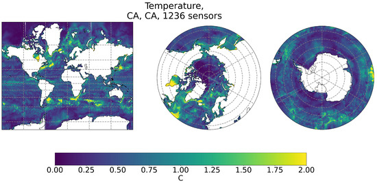
Figure 13.
Spatial distribution of reconstruction RMSE by the Concrete Autoencoder (CA) from 1236 measurements.
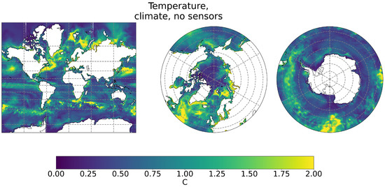
Figure 14.
Spatial distribution of reconstruction RMSE by climate without measurements.
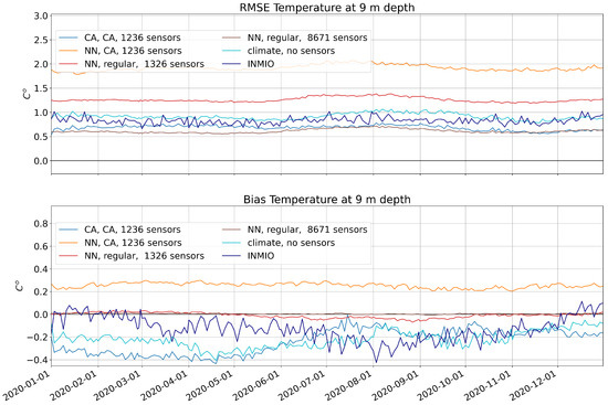
Figure 15.
The accuracy of temperature field reconstruction against the original reanalysis data is shown for the Concrete Autoencoder (CA), climate, and for Nearest Neighbor (NN) reconstruction and for different sensor placement methods. The RMSE and bias time series are based on data from the test dataset. The accuracy of reanalysis (INMIO) against ARGO float measurements is also shown.

Table 1.
Accuracy of the temperature field reconstruction at 9 m for different sensor placement methods.
We show the spatial distribution of the reconstruction bias and RMSE by the Concrete Autoencoder with 1236 measurements in Figure 11 and Figure 13 and from the climate without measurements in Figure 12 and Figure 14. The spatial distribution of errors by the Concrete Autoencoder is significantly better for the entire Pacific Ocean. In the Indian Ocean, there is a difference, but it is not as drastic. For the Gulf Stream, Kurosio, Brazil, and Circumpolar currents, the CA errors become generally smaller in comparison to the climate, but the maximum values are approximately preserved.
To demonstrate the interannual variability of reconstruction accuracy, we constructed a graph of the bias and RMSE for every second day throughout 2020 from the test set. Figure 15 indicates that the temporal patterns of RMSE remain largely unchanged for the various reconstruction methods that employ different numbers of sensors. The accuracy of the reanalysis compared to real observation data is given as an example, and it should be noted that the accuracy of the reanalysis is calculated for a limited number of measurements corresponding to the number of daily ARGO float profiles, about 300, and not for the entire computational domain as for other methods.
In Table 1, the accuracy statistics for the temperature field reconstruction are presented. The reconstruction accuracy by climate is worse in RMSE, than the proposed field reconstruction method using the Concrete Autoencoder. Moreover, the Concrete Autoencoder requires about seven times fewer sensors to achieve approximately the same accuracy as reconstruction with the Nearest Neighbor method. With the same number of sensors, the accuracy of the reconstruction with the Concrete Autoencoder is better than recovery with the Nearest Neighbor. The comparison is made according to the RMSE metric because, although for the Nearest Neighbor, the bias turns out to be very small, on average, over the entire Global ocean, there are often large deviations of different signs near a particular sensor, Figure A8, and in this case, the bias is not suitable to use for comparison. It is also important to note that the accuracy metrics for the INMIO reanalysis (test dataset) are calculated in comparison to the ARGO observation data. The number of sensors, in this case, varies within the range of 300 to 400 and is subject to daily fluctuations. Thus, the Concrete Autoencoder could reconstruct the geophysical field from a small number of sensors better than climate and, in terms of accuracy, it is close to state-of-the-art system of operational ocean forecasting [55,56,57].
4.5. Sensitivity Analysis for Sensor Measurements
For several sensor coordinates obtained by the CA method, mutual information and sensitivity fields were calculated. The most representative fields are shown in Figure 16 and Figure 17, displaying the influence of one point on the global ocean, and in Figure 18, displaying the influence of two different points on a local area.
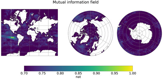
Figure 16.
Mutual information field for the temperature at 9 m from the training dataset.
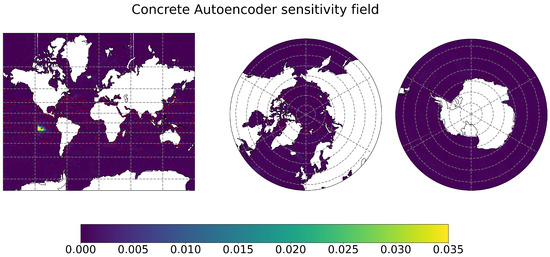
Figure 17.
Sensitivity field of the Concrete Autoencoder for the temperature at 9 m from the training dataset.
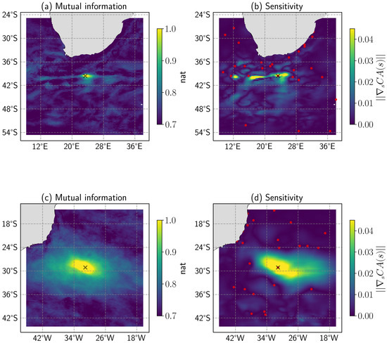
Figure 18.
Mutual information (a,c) and sensitivity of the Concrete Autoencoder (b,d) fields for the point at the front of Agulhas and Antarctic Circumpolar currents (a,b) and for the point at the Brazil current (c,d).
In Figure 16, the mutual information shows the influence of one point on distant areas in the ocean. This effect may be due to the subtraction of monthly averaged climate values, which may not be sufficient to negate the global effect of the sun and atmosphere. In Figure 17, the sensitivity field shows a more locally influenced area with a sharp left border because the point is close to the left part of the calculation domain where the periodic boundary condition is set, and the CA model does not recognize the geographical proximity of the area on the other side of the calculation domain. This results in a sensitivity pattern that is clipped on one side. A potential solution to this issue could be achieved by augmenting the training set by shifting the fields along the longitudes. This would result in the output of the Concrete Autoencoder being invariant with respect to these shifts.
In Figure 18a,b, the influence of a point close to the front of the Agulhas and Antarctic Circumpolar currents on a local area is shown. Filamentous structures, where the model is insensitive to changes in a given sensor measurement, are typically located near other sensors.
In Figure 18c,d, the influence of a point located in the wide Brazil current is shown, explaining the significant size of the spot for the mutual information and sensitivity fields. It is also clear that in areas without sensors, the sensitivity pattern is similar to the field of mutual information.
5. Discussion
In this study, we focused on regions with high information entropy, which indicates a high degree of uncertainty. By comparing the information entropy field with maps of ocean currents, we found that these regions tend to be located near the fronts between cold and warm currents. However, not all regions where cold and warm currents mix correspond to high information entropy values. Future research may investigate these regions to identify the factors that contribute to high uncertainty in some areas but not in others. This could help us better understand the relationship between the mixing of cold and warm currents and uncertainty in the ocean state.
A unique feature of the proposed method for sensor placement and field reconstruction is its ability to adjust the number of sensors during the Concrete Autoencoder training. By choosing different checkpoints of the Concrete Autoencoder, we can balance the number of sensors and the reconstruction accuracy. The results of this study showed that reducing the number of sensors below the optimal value leads to rapid error growth. Therefore, this method can be used to determine the minimum acceptable number of sensors and provide the optimal placement strategy.
The sensitivity of the Concrete Autoencoder can be used as an approximation of the mutual information field, which also takes into account the joint influence of other sensors. Investigating the sensitivity fields of the Concrete Autoencoder could also improve the interpretability of the obtained sensor locations. This sensitivity analysis tool could have several important applications. First, when placing a new observation station, it is important to find an area in which the values of the measured physical field will correlate with the values obtained at the location of this station. A system of sensors with non-overlapping areas of influence will be more cost-effective and will provide high accuracy with a minimum number of sensors. Secondly, sensitivity analysis tools are also important in numerical simulations, such as for optimizing data assimilation methods in global ocean circulation models with ensemble Kalman filters. As the number of satellite observations grows, it is important to find a balance between the amount of assimilated data and the speed of the data assimilation algorithm, which is limited by the speed of calculating the Singular Value Decomposition in ensemble Kalman filters. By using the sensor area of the influence calculation method, we can exclude sensors with significantly overlapping areas of influence from the data assimilation process, which can significantly speed up the calculation of the ocean model without sacrificing the accuracy of the forecast. In general, further investigation of the sensitivity field using the Concrete Autoencoder could provide valuable insights into the relationship between sensor placement and mutual information fields and help us better understand the factors that influence the accuracy of field reconstruction from sparse measurements.
6. Conclusions
In this paper, we propose a method for determining the optimal placement of sensors and reconstructing ocean temperature fields from sparse measurements. The results of this study demonstrate that the information entropy field has a clear correspondence with the hydrophysical features of real ocean currents. The proposed method demonstrates superiority over baseline techniques, achieving accuracy comparable to simpler reconstruction methods with up to six times fewer sensors and approaching the accuracy of the world’s state-of-the-art operational ocean forecasting systems. The method scales well for grids with at least cells, with a computational complexity that increases linearly with the number of cells. Further, comparative analysis showed that the sensitivity of the Concrete Autoencoder to disturbing a particular sensor is in good agreement with the field of mutual information of the corresponding point. This gives a good approximation of the area of influence of that sensor.
In conclusion, the presented method exhibits high reconstruction accuracy and potential for scalability. Further research may contribute to the development of an optimal ocean observing network for multiple fields and higher-resolution grids.
Author Contributions
Conceptualization, K.V.U., A.A.L. and N.A.T.; methodology, A.A.L. and N.A.T.; software, R.A.I., M.N.K., K.V.U., N.A.T. and A.A.L.; validation, N.A.T. and A.A.L.; formal analysis, K.V.U., A.A.L. and N.A.T.; investigation, A.A.L. and N.A.T.; resources, R.A.I., A.A.L. and N.A.T.; data curation, N.A.T. and A.A.L.; writing—original draft preparation, A.A.L. and N.A.T.; writing—review and editing, K.V.U.; visualization, N.A.T. and A.A.L.; supervision, R.A.I.; project administration, N.A.T.; funding acquisition, R.A.I. and A.A.L. All authors have read and agreed to the published version of the manuscript.
Funding
This research was funded by the state assignment of IO RAS, theme FMWE-2021-0003 (the test set calculation, the information entropy ensemble calculation, analysis of the temperature fields, final experiments and assessment of reconstruction accuracy for the considered optimal sensor placement methods, experiments with the mutual information), and by the BASIS Foundation, Grant No. 19-1-1-48-1 (experiments with the Concrete Autoencoder on high-resolution grids, analysis of the training dynamics at the sensor sparsification stage and computation of the sensitivity fields).
Institutional Review Board Statement
Not applicable.
Informed Consent Statement
Not applicable.
Data Availability Statement
The data presented in this study are available upon request from the corresponding authors.
Acknowledgments
The research was carried out using supercomputer resources at the Joint Supercomputer Center of the Russian Academy of Sciences (JSCC RAS), Marchuk Institute of Numerical Mathematics of the Russian Academy of Sciences (INM RAS), Moscow Institute of Physics and Technology (MIPT) and Zhores HPC [58].
Conflicts of Interest
The authors declare no conflict of interest. The funders had no role in the design of the study; in the collection, analyses, or interpretation of data; in the writing of the manuscript; or in the decision to publish the results.
Abbreviations
The following abbreviations are used in this article:
| CA | Concrete Autoencoder |
| IE | Information Entropy |
| GAN | Generative Adversarial Network |
| MI | Mutual Information |
| NN | Nearest Neighbor |
| Probability Distribution Function | |
| PixelCNN | Pixel Convolutional Neural Network |
| RMSE | Root Mean Square Error |
| SVD | Singular Value Decomposition |
Appendix A
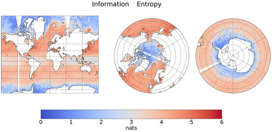
Figure A1.
Information entropy field of the temperature at 9 m depth.
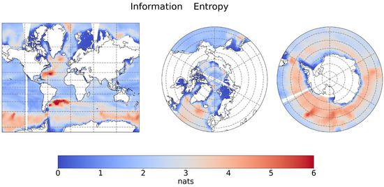
Figure A2.
Information entropy field of the temperature at 1250 m depth.
Appendix B

Figure A3.
Locations of 8671 sensors regularly placed.
Appendix C
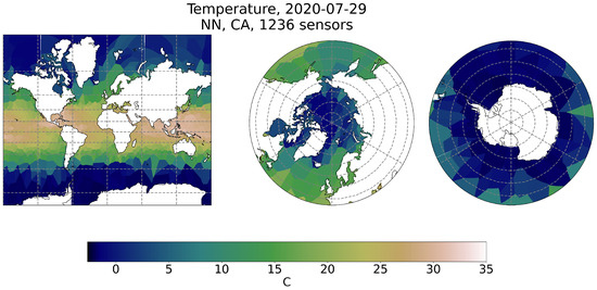
Figure A4.
Reconstructed field by the Nearest Neighbor (NN) method from 1236 measurements with placement using the Concrete Autoencoder (CA).
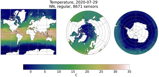
Figure A5.
Reconstructed field by the Nearest Neighbor (NN) method from 8671 measurements with regular placement.
Appendix D
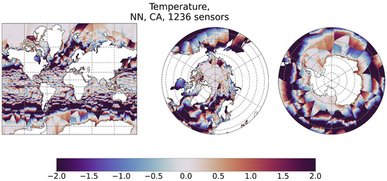
Figure A6.
Spatial distribution of reconstruction bias by the Nearest Neighbor (NN) method from 1236 measurements with placement using the Concrete Autoencoder (CA).
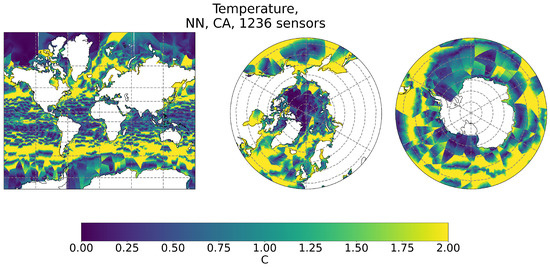
Figure A7.
Spatial distribution of reconstruction RMSE by the Nearest Neighbor (NN) method from 1236 measurements with placement using the Concrete Autoencoder (CA).
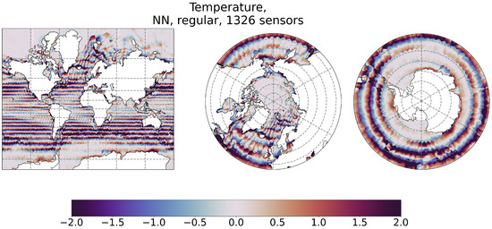
Figure A8.
Spatial distribution of reconstruction bias by the Nearest Neighbor (NN) method from 1326 measurements with regular placement.
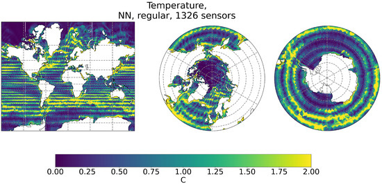
Figure A9.
Spatial distribution of reconstruction RMSE by the Nearest Neighbor (NN) method from 1236 measurements with regular placement.
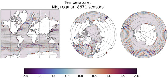
Figure A10.
Spatial distribution of reconstruction bias by the Nearest Neighbor (NN) method from 8671 measurements with regular placement.
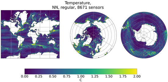
Figure A11.
Spatial distribution of reconstruction RMSE by the Nearest Neighbor (NN) method from 8671 measurements with regular placement.
References
- Tan, Y.; Zhang, L. Computational methodologies for optimal sensor placement in structural health monitoring: A review. Struct. Health Monit. 2020, 19, 1287–1308. [Google Scholar] [CrossRef]
- Mankad, J.; Natarajan, B.; Srinivasan, B. Integrated approach for optimal sensor placement and state estimation: A case study on water distribution networks. ISA Trans. 2022, 123, 272–285. [Google Scholar] [CrossRef] [PubMed]
- Inoue, T.; Ikami, T.; Egami, Y.; Nagai, H.; Naganuma, Y.; Kimura, K.; Matsuda, Y. Data-driven optimal sensor placement for high-dimensional system using annealing machine. Mech. Syst. Signal Process. 2023, 188, 109957. [Google Scholar] [CrossRef]
- Roemmich, D.; Johnson, G.C.; Riser, S.; Davis, R.; Gilson, J.; Owens, W.B.; Garzoli, S.L.; Schmid, C.; Ignaszewski, M. The Argo Program: Observing the Global Ocean with Profiling Floats. Oceanography 2009, 22, 34–43. [Google Scholar] [CrossRef]
- Cole, R.; Kinder, J.; Yu, W.; Ning, C.L.; Wang, F.; Chao, Y. Ocean Climate Monitoring. Front. Mar. Sci. 2019, 6, 503. [Google Scholar] [CrossRef]
- She, J.; Allen, I.; Buch, E.; Crise, A.; Johannessen, J.A.; Le Traon, P.Y.; Lips, U.; Nolan, G.; Pinardi, N.; Reißmann, J.H.; et al. Developing European operational oceanography for Blue Growth, climate change adaptation and mitigation, and ecosystem-based management. Ocean. Sci. 2016, 12, 953–976. [Google Scholar] [CrossRef]
- Nakai, K.; Yamada, K.; Nagata, T.; Saito, Y.; Nonomura, T. Effect of objective function on data-driven greedy sparse sensor optimization. IEEE Access 2021, 9, 46731–46743. [Google Scholar] [CrossRef]
- Clark, E.; Askham, T.; Brunton, S.L.; Nathan Kutz, J. Greedy Sensor Placement With Cost Constraints. IEEE Sens. J. 2019, 19, 2642–2656. [Google Scholar] [CrossRef]
- Saito, Y.; Nonomura, T.; Yamada, K.; Nakai, K.; Nagata, T.; Asai, K.; Sasaki, Y.; Tsubakino, D. Determinant-based fast greedy sensor selection algorithm. IEEE Access 2021, 9, 68535–68551. [Google Scholar] [CrossRef]
- Wolf, P.; Moura, S.; Krstic, M. On optimizing sensor placement for spatio-temporal temperature estimation in large battery packs. In Proceedings of the 2012 IEEE 51st IEEE Conference on Decision and Control (CDC), Grand Wailea Maui, HI, USA, 10–13 December 2012; IEEE: Piscataway, NJ, USA, 2012; pp. 973–978. [Google Scholar]
- Kumar, P.; El Sayed, Y.M.; Semaan, R. Optimized sensor placement using stochastic estimation for a flow over a 2D airfoil with Coanda blowing. In Proceedings of the 7th AIAA Flow Control Conference, Atlanta, GA, USA, 16–20 June 2014; p. 2101. [Google Scholar]
- Krause, A.; Singh, A.; Guestrin, C. Near-optimal sensor placements in Gaussian processes: Theory, efficient algorithms and empirical studies. J. Mach. Learn. Res. 2008, 9, 235–284. [Google Scholar]
- Nguyen, L.V.; Hu, G.; Spanos, C.J. Efficient sensor deployments for spatio-temporal environmental monitoring. IEEE Trans. Syst. Man Cybern. Syst. 2018, 50, 5306–5316. [Google Scholar] [CrossRef]
- Nagata, T.; Nonomura, T.; Nakai, K.; Yamada, K.; Saito, Y.; Ono, S. Data-driven sparse sensor selection based on A-optimal design of experiment with ADMM. IEEE Sens. J. 2021, 21, 15248–15257. [Google Scholar] [CrossRef]
- Ge, T.; Pathak, J.; Subramaniam, A.; Kashinath, K. DL-Corrector-Remapper: A grid-free bias-correction deep learning methodology for data-driven high-resolution global weather forecasting. arXiv 2022, arXiv:2210.12293. [Google Scholar] [CrossRef]
- Jang, E.; Gu, S.; Poole, B. Categorical Reparameterization with Gumbel-Softmax. arXiv 2016, arXiv:1611.01144. [Google Scholar] [CrossRef]
- Maddison, C.J.; Mnih, A.; Teh, Y.W. The Concrete Distribution: A Continuous Relaxation of Discrete Random Variables. arXiv 2016, arXiv:1611.00712. [Google Scholar] [CrossRef]
- Abid, A.; Balin, M.F.; Zou, J. Concrete Autoencoders for Differentiable Feature Selection and Reconstruction. arXiv 2019, arXiv:1901.09346. [Google Scholar] [CrossRef]
- Wang, Z.K.; Yang, Z.B.; Wu, S.M.; Li, H.Q.; Tian, S.H.; Chen, X.F. Optimization and assessment of blade tip timing probe layout with concrete autoencoder and reconstruction error. Appl. Soft Comput. 2022, 119, 108590. [Google Scholar] [CrossRef]
- Huijben, I.A.; Veeling, B.S.; van Sloun, R.J. Deep probabilistic subsampling for task-adaptive compressed sensing. In Proceedings of the International Conference on Learning Representations, Virtual, 25–29 April 2020. [Google Scholar]
- Singh, J.; Bagga, S.; Kaur, R. Software-based Prediction of Liver Disease with Feature Selection and Classification Techniques. Procedia Comput. Sci. 2020, 167, 1970–1980. [Google Scholar] [CrossRef]
- Williams, J.; Zahn, O.; Kutz, J.N. Data-driven sensor placement with shallow decoder networks. arXiv 2022, arXiv:2202.05330. [Google Scholar]
- Turko, N.; Lobashev, A.; Ushakov, K.; Kaurkin, M.; Ibrayev, R. Information Entropy Initialized Concrete Autoencoder for Optimal Sensor Placement and Reconstruction of Geophysical Fields. arXiv 2022, arXiv:2206.13968. [Google Scholar] [CrossRef]
- Van Oord, A.; Kalchbrenner, N.; Kavukcuoglu, K. Pixel recurrent neural networks. In Proceedings of the International Conference on Machine Learning, New York, NY, USA, 20–22 June 2016; pp. 1747–1756. [Google Scholar]
- Van den Oord, A.; Kalchbrenner, N.; Espeholt, L.; Vinyals, O.; Graves, A. Conditional image generation with pixelcnn decoders. arXiv 2016, arXiv:1606.05328. [Google Scholar] [CrossRef]
- Ronneberger, O.; Fischer, P.; Brox, T. U-net: Convolutional networks for biomedical image segmentation. In Proceedings of the International Conference on Medical Image Computing and Computer-Assisted Intervention, Munich, Germany, 5–9 October 2015; Springer: Cham, Switzerland, 2015; pp. 234–241. [Google Scholar]
- Bengio, Y.; Léonard, N.; Courville, A. Estimating or propagating gradients through stochastic neurons for conditional computation. arXiv 2013, arXiv:1308.3432. [Google Scholar]
- Isola, P.; Zhu, J.Y.; Zhou, T.; Efros, A.A. Image-to-image translation with conditional adversarial networks. In Proceedings of the IEEE Conference on Computer Vision and Pattern Recognition, Honolulu, HI, USA, 21–26 July 2017; pp. 1125–1134. [Google Scholar]
- Kraskov, A.; Stogbauer, H.; Grassberger, P. Estimating mutual information. Phys. Rev. E 2004, 69, 066138. [Google Scholar] [CrossRef]
- Dafydd, E. A computationally efficient estimator for mutual information. Proc. R. Soc. A 2008, 464, 1203–1215. [Google Scholar] [CrossRef]
- Kalnitskii, L.; Kaurkin, M.; Ushakov, K.; Ibrayev, R. Supercomputer Implementation of a High Resolution Coupled Ice-Ocean Model for Forecasting the State of the Arctic Ocean. In Supercomputing. RuSCDays 2020; Communications in Computer and Information Science; Voevodin, V., Sobolev, S., Eds.; Springer: Cham, Switzerland, 2020; Volume 1331. [Google Scholar] [CrossRef]
- Argo, G. Argo Float Data and Metadata from Global Data Assembly Centre (Argo GDAC); Seanoe: Pasadena, CA, USA, 2000. [Google Scholar]
- Desai, S. Jason-3 GPS based orbit and SSHA OGDR. In NASA Physical Oceanography DAAC; PO.DAAC: Pasadena, CA, USA, 2016. [Google Scholar] [CrossRef]
- Lavergne, T.; Sørensen, A.M.; Kern, S.; Tonboe, R.; Notz, D.; Aaboe, S.; Bell, L.; Dybkjær, G.; Eastwood, S.; Gabarro, C.; et al. Version 2 of the EUMETSAT OSI SAF and ESA CCI sea-ice concentration climate data records. Cryosphere 2019, 13, 49–78. [Google Scholar] [CrossRef]
- Masina, S.; Cipollone, A.; Iovino, D.; Ciliberti, S.; Coppini, G.; Lecci, R.; Creti, S.; Palermo, F.; Viola, F.; Lyubartsev, V.; et al. A Global Ocean Eddying Forecasting System at 1/16°. In Proceedings of the 9th EuroGOOS International Conference, Online, 3–5 May 2021. [Google Scholar]
- Bryan, K. A numerical method for the study of the circulation of the world ocean. J. Comput. Phys. 1997, 135, 154–169. [Google Scholar] [CrossRef]
- Lebedev, V.I. Difference analogues of orthogonal decompositions, basic differential operators and some boundary problems of mathematical physics. I. USSR Comput. Math. Math. Phys. 1964, 4, 69–92. [Google Scholar] [CrossRef]
- Lebedev, V.I. Difference analogues of orthogonal decompositions, basic differential operators and some boundary problems of mathematical physics. II. USSR Comput. Math. Math. Phys. 1964, 4, 36–50. [Google Scholar] [CrossRef]
- Mesinger, F.; Arakawa, A. Numerical Methods Used in Atmospheric Models; GARP Publication Series No. 17; World Meteorological Organization: Geneva, Switzerland, 1976. [Google Scholar]
- Ushakov, K.; Ibrayev, R. Assessment of mean world ocean meridional heat transport characteristics by a high-resolution model. Russ. J. Earth Sci. 2018, 18, ES1004. [Google Scholar] [CrossRef]
- Hunke, E.C.; Lipscomb, W.H.; Turner, A.K.; Jeffery, N.; Elliott, S. CICE: The Los Alamos Sea Ice Model, Documentation and Software User’s Manual, Version 5.1 la-cc-06-012; Los Alamos National Laboratory: Los Alamos, NM, USA, 2010; Volume 675, p. 500.
- Killworth, P.D.; Webb, D.J.; Stainforth, D.; Paterson, S.M. The development of a free-surface Bryan–Cox–Semtner ocean model. J. Phys. Oceanogr. 1991, 21, 1333–1348. [Google Scholar] [CrossRef]
- Griffies, S.M.; Hallberg, R.W. Biharmonic friction with a Smagorinsky-like viscosity for use in large-scale eddy-permitting ocean models. Mon. Weather Rev. 2000, 128, 2935–2946. [Google Scholar] [CrossRef]
- Munk, W.H. Note on the theory of the thermocline. J. Mar. Res. 1948, 7, 276–295. [Google Scholar]
- Griffies, S.M.; Biastoch, A.; Boning, C.; Bryan, F.; Danabasoglu, G.; Chassignet, E.P.; England, M.H.; Gerdes, R.; Haak, H.; Hallberg, R.W.; et al. Coordinated ocean-ice reference experiments (COREs). Ocean. Model. 2009, 26, 1–46. [Google Scholar] [CrossRef]
- Hersbach, H.; Bell, B.; Berrisford, P.; Hirahara, S.; Horányi, A.; Muñoz-Sabater, J.; Nicolas, J.; Peubey, C.; Radu, R.; Schepers, D.; et al. The ERA5 global reanalysis. Q. J. R. Meteorol. Soc. 2020, 146, 1999–2049. [Google Scholar] [CrossRef]
- Kaurkin, M.N.; Ibrayev, R.A.; Belyaev, K.P. Data assimilation in the ocean circulation model of high spatial resolution using the methods of parallel programming. Russ. Meteorol. Hydrol. 2016, 41, 479–486. [Google Scholar] [CrossRef]
- Kaurkin, M.; Ibrayev, R.; Koromyslov, A. EnOI-Based Data Assimilation Technology for Satellite Observations and ARGO Float Measurements in a High Resolution Global Ocean Model Using the CMF Platform. In Supercomputing. RuSCDays 2016; Communications in Computer and Information Science; Voevodin, V., Sobolev, S., Eds.; Springer: Cham, Switzerland, 2016; Volume 687. [Google Scholar] [CrossRef]
- Evensen, G. Data Assimilation; Springer: Berlin/Heidelberg, Germany, 2009. [Google Scholar] [CrossRef]
- Ryan, A.; Regnier, C.; Divakaran, P.; Spindler, T.; Mehra, A.; Smith, G.; Davidson, F.; Hernandez, F.; Maksymczuk, J.; Liu, Y. GODAE OceanView Class 4 forecast verification framework: Global ocean inter-comparison. J. Oper. Oceanogr. 2015, 8, s98–s111. [Google Scholar] [CrossRef]
- Manohar, K.; Brunton, B.W.; Kutz, J.N.; Brunton, S.L. Data-driven sparse sensor placement for reconstruction: Demonstrating the benefits of exploiting known patterns. IEEE Control Syst. Mag. 2018, 38, 63–86. [Google Scholar]
- Randelhoff, A.; Reigstad, M.; Chierici, M.; Sundfjord, A.; Ivanov, V.; Cape, M.; Vernet, M.; Tremblay, J.E.; Bratbak, G.; Kristiansen, S. Seasonality of the physical and biogeochemical hydrography in the inflow to the Arctic Ocean through Fram Strait. Front. Mar. Sci. 2018, 5, 224. [Google Scholar] [CrossRef]
- Roxy, M.K.; Gnanaseelan, C.; Parekh, A.; Chowdary, J.S.; Singh, S.; Modi, A.; Kakatkar, R.; Mohapatra, S.; Dhara, C.; Shenoi, S.C.; et al. Indian Ocean Warming. In Assessment of Climate Change over the Indian Region: A Report of the Ministry of Earth Sciences (MoES), Government of India; Krishnan, R., Sanjay, J., Gnanaseelan, C., Mujumdar, M., Kulkarni, A., Chakraborty, S., Eds.; Springer: Singapore, 2020; pp. 191–206. [Google Scholar] [CrossRef]
- Inoue, M.; Takehara, R.; Yamashita, S.; Senjyu, T.; Morita, T.; Miki, S.; Nagao, S. Convection of surface water in the northeastern Japan Sea: Implications from vertical profiles of 134Cs concentrations. Mar. Chem. 2019, 214, 103661. [Google Scholar] [CrossRef]
- Carvalho, J.P.S.; Costa, F.B.; Mignac, D.; Tanajura, C.A.S. Assessing the extended-range predictability of the ocean model HYCOM with the REMO ocean data assimilation system (RODAS) in the South Atlantic. J. Oper. Oceanogr. 2021, 14, 13–23. [Google Scholar] [CrossRef]
- Lea, D.J.; While, J.; Martin, M.J.; Weaver, A.; Storto, A.; Chrust, M. A new global ocean ensemble system at the Met Office: Assessing the impact of hybrid data assimilation and inflation settings. Q. J. R. Meteorol. Soc. 2022, 148, 1996–2030. [Google Scholar] [CrossRef]
- Schiller, A.; Brassington, G.B.; Oke, P.; Cahill, M.; Divakaran, P.; Entel, M.; Freeman, J.; Griffin, D.; Herzfeld, M.; Hoeke, R.; et al. Bluelink ocean forecasting Australia: 15 years of operational ocean service delivery with societal, economic and environmental benefits. J. Oper. Oceanogr. 2020, 13, 1–18. [Google Scholar] [CrossRef]
- Zacharov, I.; Arslanov, R.; Gunin, M.; Stefonishin, D.; Bykov, A.; Pavlov, S.; Panarin, O.; Maliutin, A.; Rykovanov, S.; Fedorov, M. “Zhores”—Petaflops supercomputer for data-driven modeling, machine learning and artificial intelligence installed in Skolkovo Institute of Science and Technology. Open Eng. 2019, 9, 512–520. [Google Scholar] [CrossRef]
Disclaimer/Publisher’s Note: The statements, opinions and data contained in all publications are solely those of the individual author(s) and contributor(s) and not of MDPI and/or the editor(s). MDPI and/or the editor(s) disclaim responsibility for any injury to people or property resulting from any ideas, methods, instructions or products referred to in the content. |
© 2023 by the authors. Licensee MDPI, Basel, Switzerland. This article is an open access article distributed under the terms and conditions of the Creative Commons Attribution (CC BY) license (https://creativecommons.org/licenses/by/4.0/).