Impacts of High-Density Suspended Aquaculture on Water Currents: Observation and Modeling

Abstract

Large-scale aquaculture activities in China have been rapidly developing in coastal waters, and they inevitably affect hydrodynamic structures and, hence, substance transportation. Predicting the effects is critical for understanding the environmental ecology and biochemical processes in these waters. To realize the solution, we conducted a field observation in Sungo Bay, which is an important aquaculture bay in China, and we developed a three-dimensional numerical model by arranging so-called porous structures, representing the aquaculture facilities, on grids of the culture layers. The energy-loss coefficients were specified to determine the momentum loss by the friction of the structures. We determined the appropriate coefficients for the oyster, scallop, and kelp cultures by using numerical simulation. According to the observation and model results, the aquaculture substantially weakened the current velocities in the culture layers and altered the vertical structures of the water currents. For this high-density and large-scale culture bay, the decrease rates of the current velocities in the culture layer were up to ~68%, ~65% and ~60% in the culture zones of oysters, scallops, and kelps, respectively. Bivalve cultures and kelp and bivalve cultures reduced the water-exchange ability of the bay by 33% and 50%, respectively. The method and results of this study provide a reference for studies on other aquaculture bays.

1. Introduction

In recent decades, aquaculture has been rapidly developing in the coastal waters of China, which is the only country where the production volume from mariculture exceeds that from marine capture [1]. The area and production of mariculture in China increased from ~4.5 × 10⁵ ha (1 ha = 10⁴ m²) and ~1.9 × 10⁶ t in 1991, respectively, to 2.1 × 10⁶ ha and 1.5 × 10⁷ t in 2010 [2], respectively, accounting for ~80% of the world’s total mariculture production [1]. At present, 84.5% of the worldwide production originates from China [3]. In China, the main organisms of aquaculture are macroalgae, shellfish, shrimps, and fish, which are produced from suspension culture (longline rafts and cages) in the water column, or from bottom-sowing culture in shallow water and intertidal zones [4,5]. However, intensive aquaculture has had negative impacts on the ecological environments of many Chinese bays, where the massive and dense suspension culture has reduced water flows, which has resulted in water eutrophication, hypoxia, and the increased mortality of culture species [6,7,8]. As a scientific support, we need to assess the carrying capacity for sustainable aquaculture by integrating the ecological model [9,10,11]. To do so, investigating the impacts of aquaculture on the hydrodynamic processes and substance exchange is a prerequisite, because massive mariculture facilities and the attached species make local hydrodynamic regimes distinct [12]. Disregarding the impacts will inevitably result in a substantial overestimation of the water-renewal periods [13] and carrying capacities of culture areas [14,15].

To study the impacts of aquaculture on water currents, researchers have conducted field surveys. In Golden Bay in New Zealand, researchers studied a suspended mussel canopy and found that the current velocities in the upper water column were reduced by 43% [16]. In Whitehaven Harbor in Canada, the scallop culture caused a 40% decrease in the current velocities compared with the ambient currents [17]. According to the observation in Sungo Bay in 2001, the reduction in the velocities caused by bivalve culture was ~20% [18]. Zhu et al. [19] found that the velocities in the surface layer in this bay were reduced by 50%, on average, because of aquaculture. Grant and Bacher [20] reported that the suspended culture resulted in a 54% reduction in the speed in a culture area of this bay. Thus, previous surveys indicate that the current velocities in aquaculture waters have been significantly reduced. In recent years, high-density and large-scale aquaculture has been developed in many bays in China, such as Sungo Bay, Rongcheng Bay, Sansha Bay, and Dongshan Bay [21]. To better understand the impacts, and especially the vertical patterns of water currents, and to provide data for modeling, we need to further investigate bays that are fully occupied by aquaculture.

Numerical modeling is an essential method for predicting ecological implications and hydrodynamic regimes. However, few models have addressed the effects of aquaculture. Grant et al. [22] developed a two-dimensional circulation model to define the frictional force of aquaculture facilities, in which the friction-drag coefficient of the bivalve facilities was 23 fold the seabed-drag coefficient. Based on laboratory and numerical simulations, O’Donncha et al. [23] defined the drag coefficient of mussel facilities and set up a two-dimensional model to predict the hydrodynamics within the culture farm. Wang et al. [19] developed a two-dimensional circulation model in a kelp-culture area by incorporating the additional resistance force on the flow. Fan et al. [12] built a one-dimensional model by defining an upper boundary layer for describing the friction of aquaculture. By using this upper boundary layer, and by taking the drag coefficient of kelp as 0.025, Shi et al. [24,25] established a three-dimensional model for aquaculture water. Based on the results of laboratory experiments for the drag force, Rickard [26] developed a three-dimensional model by imposing the drag term of a fish cage on the water flow, which has not yet been used for a specific aquaculture area. Thus far, a three-dimensional model that involves the direct impacts of aquaculture on the mid-layer (the culture layer) of the water column has yet to be developed, which is a model that needs to define the aquaculture friction (or the energy loss) that is imposed on the mid-layer instead of only that imposed on the bottom or surface layers. In addition, we need to specify the appropriate drag coefficients (or the energy-loss coefficients) for different species in high-density and large-scale culture bays.

With high primary production and rich aquatic resources, Sungo Bay is an important aquaculture bay in China. Sungo Bay is in the Shandong Peninsula and is semi-enclosed and connected to the Yellow Sea, with an 11.5 km-wide mouth (Figure 1). The bay extends 7.5 km from west to east, with an average depth of 7 m. In the bay, the main species in recent years have been scallops, oysters, and kelps, which occupy most of the bay (Figure 1b). The total aquaculture production is ~2.635 × 10⁵ t/y [4]. This study on the impacts of aquaculture on Sungo Bay is representative. In this study, we observed the water currents in Sungo Bay to further understand the impacts of aquaculture, particularly on the vertical structures of the flow velocities, and to provide data for modeling. To numerically study the impacts, we developed a physical model by defining the so-called porous structures that produce momentum loss in water currents. We used the numerical simulation to determine the energy-loss coefficients for the oyster, scallop, and kelp cultures. We numerically evaluated the impacts of aquaculture on the water currents and substance exchange.

2. Materials and Methods

To investigate the impacts of the aquaculture facilities on the water currents, we conducted the field observation and model simulation together. We further used the observed data to construct and calibrate the models, which helped us to evaluate the impacts and substance exchange in the aquaculture waters.

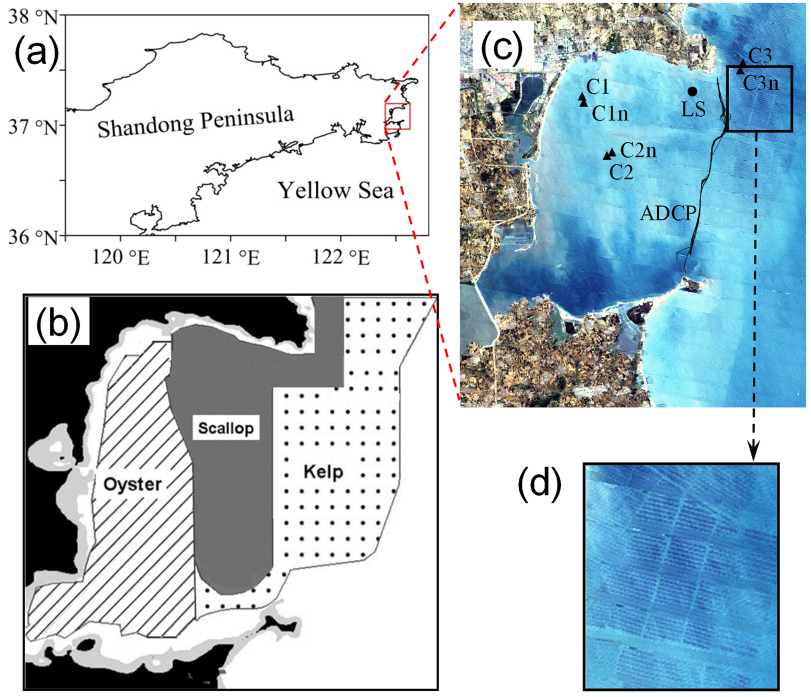
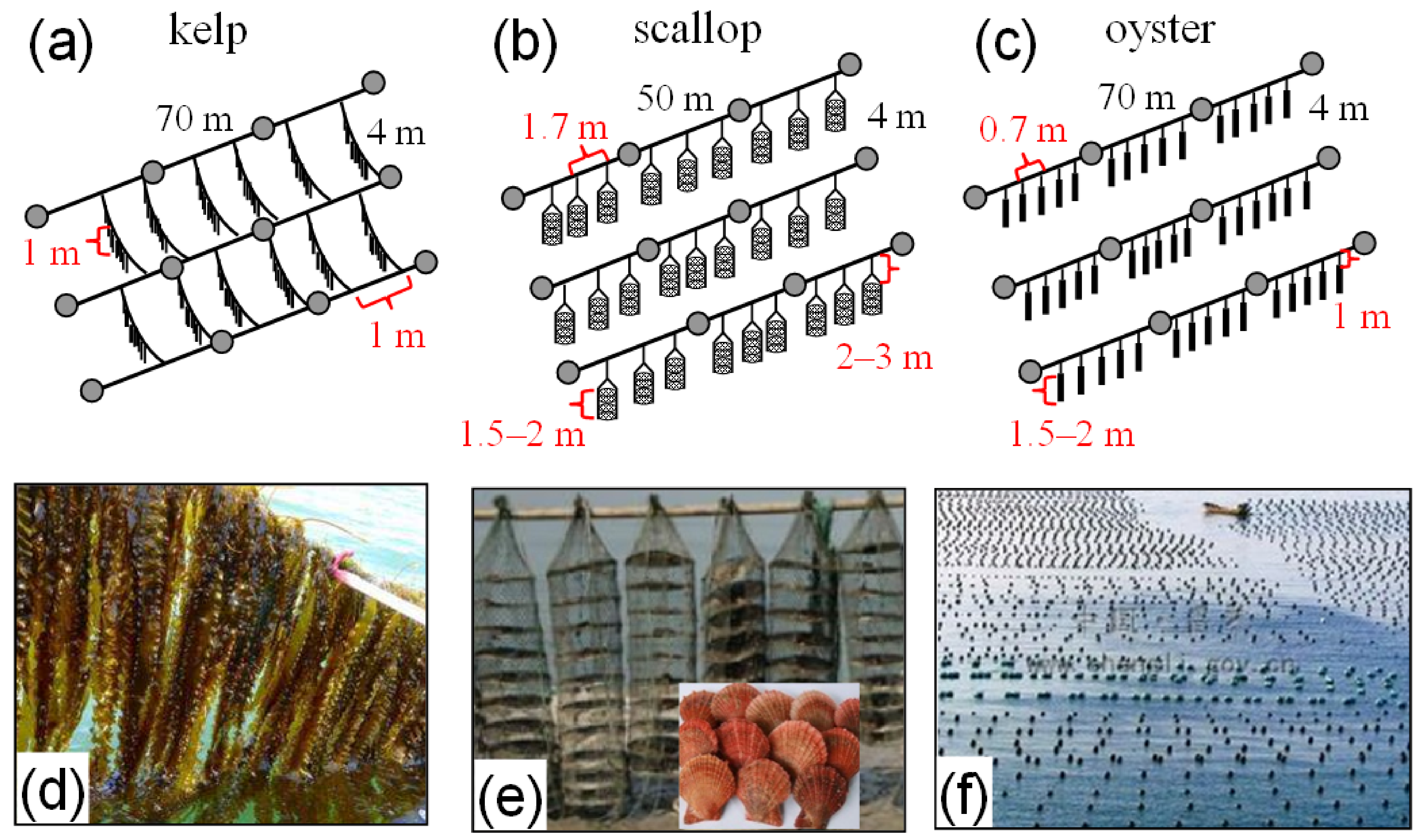
2.1. Field Observations

We used the water levels from a tidal gauge at the LS site (Figure 1c) from 20 March to 22 April 1984, when there was no intensive aquaculture, to calibrate the default model to ensure that the established primitive model was not affected by aquaculture.

We conducted the underway measurements of the water currents by using an acoustic Doppler current profiler (ADCP) at the bay mouth (Figure 1c), through the water column (from a 1.37 m depth to the bottom), with a vertical grid of 0.25 m, from 07:25 to 18:12 GMT + 8 on 7 July 2007, when there were few aquaculture facilities in the region (kelps had been harvested).

In the aquaculture areas, water currents were observed at three sites, among which Sites C1 (122.497° E, 37.133° N) and C2 (122.528° E, 37.112° N) were situated in oyster-culture zones, and Site C3 (122.595° E, 37.16° N) was in a scallop zone (Figure 1c). The currents were profiled with Compact-EM Current Meters, with a time interval of 10 min, from a 1.61 m depth to the bottom layer, with vertical grids of 0.25 m at C1, and 0.5 m at C2 and C3. At C1, water currents were observed from 10:58 to 16:48 GMT + 8 on 18 July 2007. As a comparison, we observed a nearby site, C1n (122.498° E, 37.13° N), at a distance of 339.9 m to C1, within a non-aquaculture region (200 m × 200 m), from 10:58 to 16:48 on the same day. We observed C2 from 9:20 to 17:30 on 19 July 2007, and we observed a nonculture site, C2n (122.529° E, 37.116° N), at a distance of 434.0 m to C2 from 9:40 to 18:20. We observed C3 from 9:50 to 16:50 on 22 July 2007, and we observed a nearby nonculture site, C3n (122.594° E, 37.158° N), at a distance of 216.1 m to C3 between 10:10 and 16:40 on the same day.

2.2. Method for Modeling Physical Process in the Aquaculture Bay

When flowing through culture facilities, water is subjected to their friction, which generates a loss of energy, in addition to the loss by the bottom friction. To add the friction of a culture facility to the model, we regarded the facility as so-called porous structures that produce the energy loss of water by its friction. We regarded this porous structure as a transparent structure that extends into the flow along the grid directions and covers some layers. Thus, the friction of this structure can be controlled by the quadratic friction term of a hydraulic structure, which is listed in the manual of the Delft3D Version 3.15 (Deltares, Delft, the Netherlands) model that we used in this study [28]. In the momentum Equations (1) and (2), the contributions due to the external sinks of momentum that are forced by aquaculture facilities are given by the mathematical Equations (3) and (4):

$$\frac{\partial u}{\partial t}+u\frac{\partial u}{\partial x}+v\frac{\partial u}{\partial y}+w\frac{\partial u}{\partial z} =fv-\frac{1}{\rho }\frac{\partial p}{\partial x}+\frac{\partial }{\partial z}\left(\gamma \frac{\partial u}{\partial z}\right)+M_x$$

(1)

$$\frac{\partial v}{\partial t}+u\frac{\partial v}{\partial x}+v\frac{\partial v}{\partial y}+w\frac{\partial v}{\partial z}=-fu-\frac{1}{\rho }\frac{\partial p}{\partial y}+\frac{\partial }{\partial z}\left(\gamma \frac{\partial v}{\partial z}\right)+M_y$$

(2)

$$M_x=-C_{loss-u}\frac{{\left(u^2+v^2\right)}^{\frac{1}{2}}}{\Delta x}u$$

(3)

$$M_y=-C_{loss-v}\frac{{\left(u^2+v^2\right)}^{\frac{1}{2}}}{\Delta y}v$$

(4)

where $C_{loss-u}$ and $C_{loss-v}$ are the energy-loss coefficients in the x and y directions, respectively; u and v are the velocities in the x and y directions, respectively; Δx and Δy are the lengths of the aquaculture facilities along the two orthogonal directions; w is the vertical velocity; p is water pressure at the depth (z); ρ is the water density; f is the Coriolis parameter; $\gamma$ is the viscosity coefficient.

In the numerical model, the momentum loss as a sink needs to be implemented in the grid cells that extend over one or more layer(s) of the water column, where aquaculture facilities exist. To parameterize the loss, we specified the $C_{loss-u}$ and $C_{loss-v}$ at the grid cells.

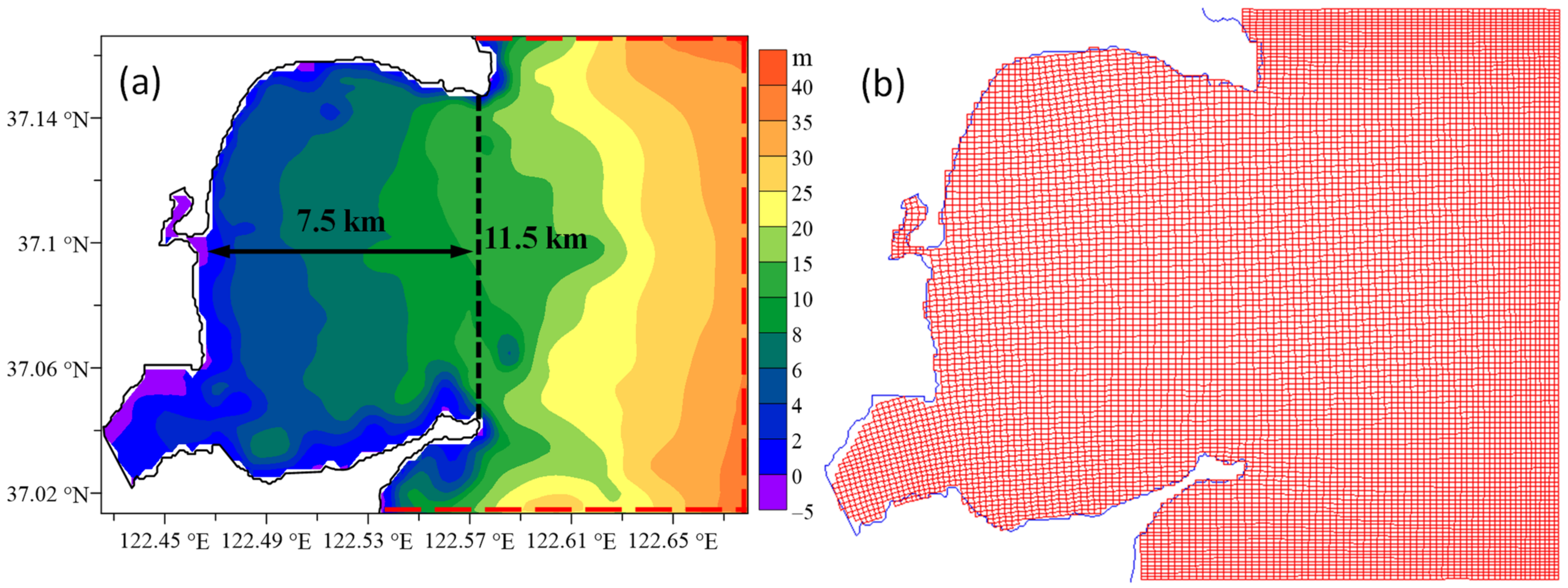
2.3. Model Configuration and Data Usage

The Delft3D-FLOW was used to simulate the hydrodynamic process of Sungo Bay. This model suite is widely used to calculate unsteady flow and transport phenomena [29], predict sandy sediment processes [30], and provide the support for environmental sustainable management [31]. Because tidal currents are the prominent physical processes in the bay [13,25] and the purpose was to study the impacts of aquaculture on water currents, we only considered tidal forces in the model using the barotropic mode. We chose the open boundaries in the open areas without aquaculture, where the water-level forcing was calculated as follows:

$$H={\displaystyle \sum }_i^4{A}_i\cos \left(w_{i}t-{\theta }_i+{\phi }_i\right)$$

(5)

where A_i, ${\theta }_i$, and ${\phi }_i$ represent the amplitude, phase lag, and initial phase of the tide constituents, respectively. The four tidal components are M₂, S₂, O₁, and K₁. The harmonic constants of them were taken from the atlas [32,33] and amended by model validation.

Figure 2 shows the model area and grids. The grids were generated and refined according to the default grid property parameters (including smoothing and orthogonality parameters) in Delft3D [28]. The bathymetry was generated through the interpolation of the topography data observed in Sungo Bay in 1999. The grid schemes have horizontal resolutions of 120 m × 120 m–220 m × 220 m. The water column was separated into six layers, which were spaced by 0.1, 0.15, 0.2, 0.2, 0.2, and 0.15 fractions of the water depth from the surface to the bottom. The time step was 180 s. The initial water levels and currents in all grid cells were set as 0.4 m and 0, respectively. The Manning formulation was used for the bed friction, with a typical Manning coefficient of 0.026 m/s^1/3 in Delft3D [28]. In the vertical direction, the k-ε turbulence model [28] was used. The horizontal eddy viscosity and diffusivity were set as 1.0 m²/s and 10.0 m²/s, respectively, and we set the vertical eddy viscosity and diffusivity as 10⁻⁶ m²/s.

The primitive default model (without aquaculture) was simulated from March to April 1984. The observed water levels at the LS site were used for the model validation.

As shown in Figure 1b, kelp, scallops, and oysters were cultured in different regions in the bay. Figure 3 shows the culture methods for these species, which are explained as follows:

Kelps: Kelps are usually longer than 1 m during most of the culture time (November–June), and their holdfasts are attached to 4 m long horizontal strings. The strings are connected by two parallel 70 m long ropes at a 1 m interval. Kelps usually float in the surface layer, which is 1 m in depth.

Scallops: Scallops are cultured in 1.5–2 m long cages below the depth of 2–3 m, which are suspended by horizontal 50 m long ropes. The interval for the ropes is 4 m, and each rope supports ~30 cages in 1.7 m intervals. The diameter of a cage is ~30 cm.

Oysters: Below the depth of 1 m, the oysters adhere to suspended strings, which occupy lengths of 1.5–2 m. The strings are hung by 70 m long ropes that have 4 m intervals (a rope hangs ~100 strings at 0.7 m intervals).

In addition, fishing-boat channels with widths of 20 m were left the among aquaculture zones.

In the model, we specified the culture layer of kelp as the first grid cell in the vertical direction; the layer of oysters was the second, third, or fourth layer according to the water depths; scallops were arranged in the second, third, fourth, second and third, or third and fourth layer(s), depending on the local depths. We added the energy losses (M_x and M_y) in the momentum Equations (1) and (2) at these grids and layer(s).

On the one hand, in this high-density and fully occupied aquaculture bay, we assumed that the aquaculture occupied all the grid cells in aquaculture zones shown in Figure 1b. On the other hand, the lengths of the aquaculture facilities (Δx and Δy) are less than the model resolutions along the two orthogonal directions. Therefore, for this dense and massive culture bay, Δx and Δy were taken as the grid-resolution lengths in the x and y directions, respectively. In addition, the scale of the horizontal-grid resolutions is much larger than the cage, and thus we did not study the local fluid dynamics of the inside of it, but we did study the effects of aquaculture on the water currents in a high-density and large-scale culture bay.

At each aquaculture cell, energy-loss coefficients ($C_{loss-u}$ and $C_{loss-v}$) were to be specified. For these porous structures, the coefficients were not available in the Delft3D model and references. Therefore, we specified the appropriate coefficients by conducting numerical simulations (i.e., approximation experiments) with observations. Even though the $C_{loss-u}$ and $C_{loss-v}$ might differ in a grid cell, we specified the same coefficients for them for a cultured species, as discovering the laying directions of the facilities in the many zones of this large-scale aquaculture bay is difficult. At the culture layers, we used an upwind approximation in the advective terms of the momentum equations to prevent or damp oscillations that might occur because of large gradients. The simulation time for the aquaculture model was July 2007.

For validation and calibration processes, the model accuracy was quantified using the root mean square error (RMSE), the scatter index (SI), and the average absolute percentage error (%Err) according to the formulas as follows [29]:

$$RMSE=\sqrt{\frac{1}{N}{{\displaystyle \sum }}_{i=1}^N{\left(p_i-m_i\right)}^2}$$

(6)

$$SI=\frac{RMSE}{\max \left(RM{S}_m, 〈\left|m\right|〉\right)}$$

(7)

$$\%Err=\frac{〈\left|p-m\right|〉}{〈\left|m\right|〉}\times 100\%$$

(8)

where p = p₁, p₂, …, p_i and m = m₁, m₂, …, m_i indicate the predicted and measured data, respectively, and RMS is the root mean square.

2.4. Modeling of Water Exchange

To evaluate the effects of the aquaculture on the water exchange, we simulated the diffusion of a conceptual conservative substance in cases of no aquaculture and aquaculture in the bay. Here, biochemical processes and land input were not considered. The diffusion equation is:

$$\frac{\partial C}{\partial t}+u\frac{\partial C}{\partial x}+v\frac{\partial C}{\partial y}+w\frac{\partial C}{\partial z}=\frac{\partial C}{\partial x}\left(A_h\frac{\partial C}{\partial x}\right)+\frac{\partial C}{\partial y}\left(A_h\frac{\partial C}{\partial y}\right)+\frac{\partial C}{\partial w}\left(A_h\frac{\partial C}{\partial z}\right)$$

(9)

where C is the material concentration, and A_h and A_v the are horizontal and vertical diffusivities, respectively. We set the initial concentration in a dimensionless unit as 1.0 for the entire model area, and the control value at the open boundary was 0. The exchange processes were simulated under the condition of middle ebb.

The half-exchange period, or the elapsed time during which the concentration decays to half of the initial value [34], was defined as the water-exchange time. In our model, after the half-exchange period, the average concentration of the inner bay (the area west of the dashed line in Figure 2a) was reduced to 0.5.

3. Results

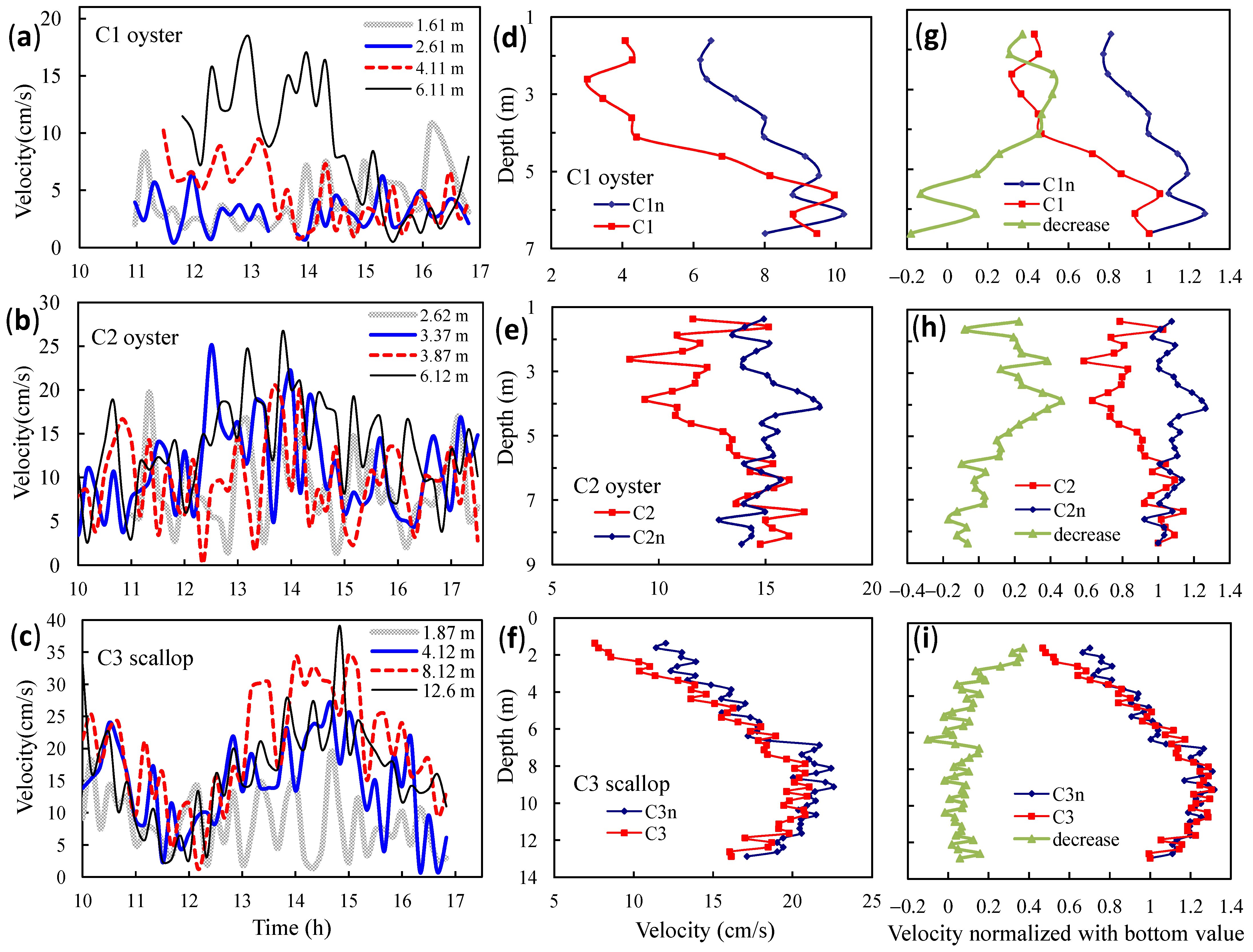
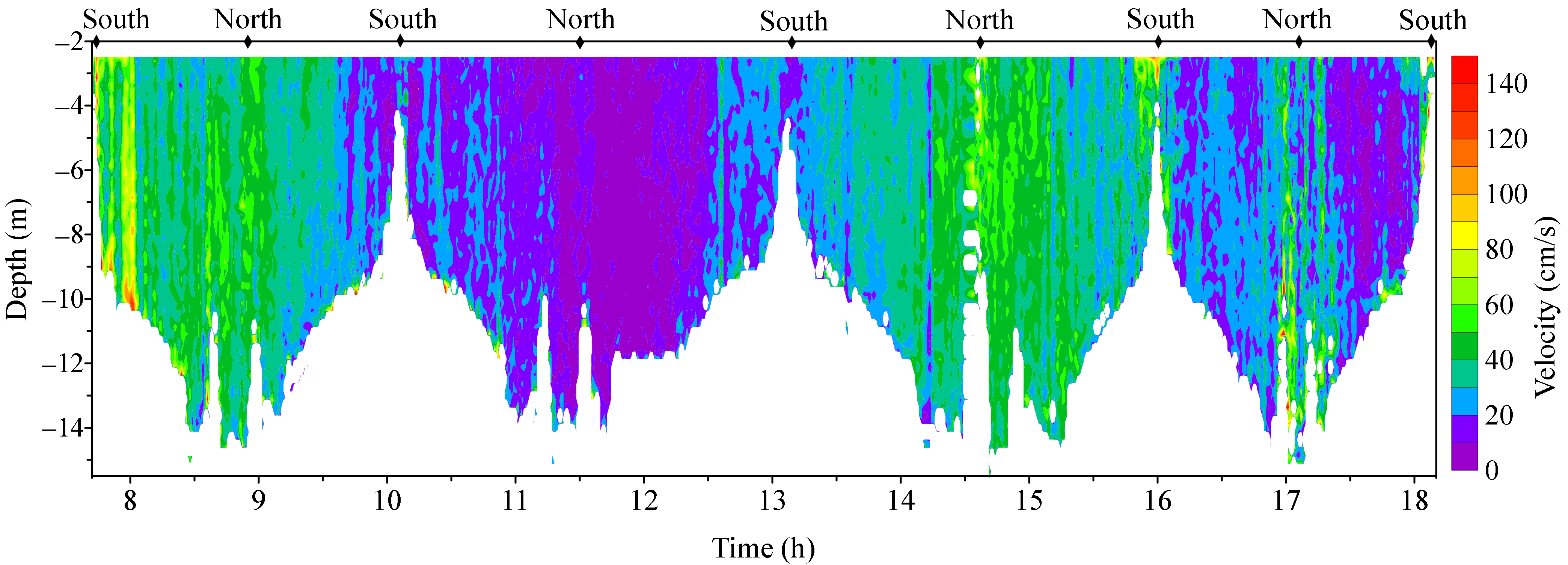
3.1. Observed Water Currents in Areas without Aquaculture

Figure 4 shows the vertical profiles (four round routes) of the water currents observed by the ADCP at the bay mouth where kelps had been harvested. We ignored the currents at depths of less than 2.5 m as the disturbances of shipping bubbles. In the non-aquaculture area, the water-current velocities in the lower layers are generally not higher than those in the upper layer. The vertical distributions of the currents in the area differ from those in the aquaculture areas shown in Figure 5.

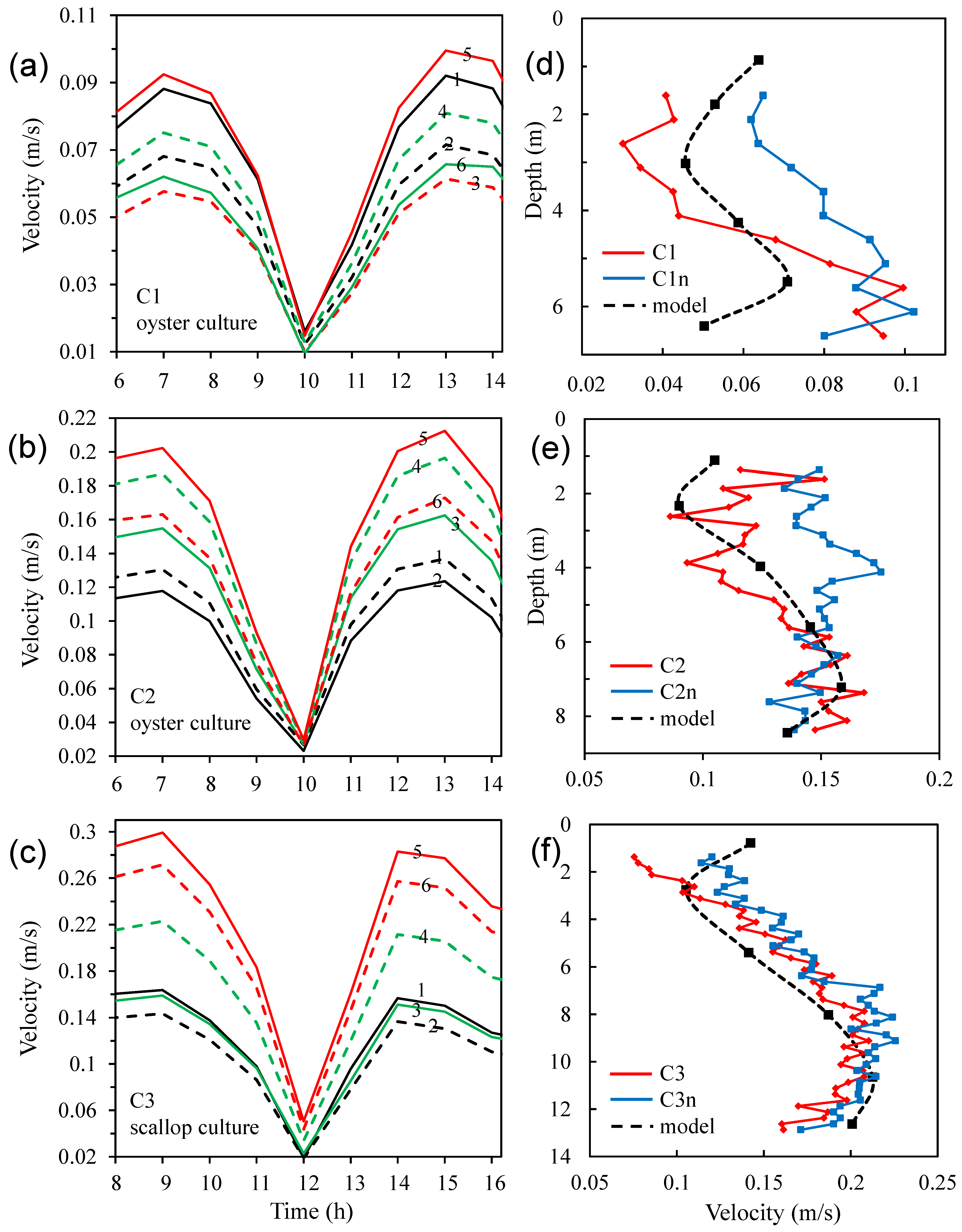
3.2. Observed Water Currents in Areas with Aquaculture

Figure 5 demonstrates water currents observed at the three sites in bivalve-culture areas, including the time series of the current velocities at typical depths, and vertical patterns of the velocities (averaged within the observation period) at the culture sites and their nearby boat channels. Figure 5g–i show the vertical patterns for the local decrease rates of the velocities (such as (V_C1n − V_C1)/V_C1n for C1, where V_C1 and V_C1n are the velocities at C1 and C1n, respectively), and for the normalized dimensionless values (the velocities divided by the near-bottom velocities, which were little affected by the aquaculture).

At C1, where oysters were cultured in a 1–3 m deep layer, the current velocities in the layer (at 1.61 m and 2.61 m depths) were generally less than those in the lower water. Compared with a nearby site (C1n) situated in a boat channel without aquaculture, the water currents were significantly reduced by the culture facilities. At a depth of 2.61 m, the velocities were 6.4 and 3.0 cm/s at C1n and C1, respectively (the decrease was ~53%), which indicates the local effect of the facilities. At C1n, the velocities in the upper layers were less than those in the lower layers (below 4.11 m), which means that the water currents in the channel were slowed by the nearby culture. At C1, the minimum of the normalized values was 0.32 (at a 2.61 m depth), which indicates that the current velocities in the culture layer in this region were reduced by ~68% by the aquaculture in the bay.

At another oyster-culture site (C2), the velocities in the culture layer were lower than those in the upper and lower layers. In the nonculture layers, the velocities at C2 were close to those at C2n (in a boat channel); however, in the culture layer, the velocities were significantly depressed by the local facilities. Compared with C2n, the maximum reduction in the velocities in the culture layer was ~40%. The normalized values were between 0.57 and 0.74 in the culture layer, which indicates that the aquaculture in the bay resulted in a decrease of 26–43% in the current velocities in the culture layer in this region.

At C3, the water currents at depths of 2–5 m, where scallops were cultured, were slower than those in the other layers. The maximal velocities appeared at 9.12 m, where the water was barely subjected to the frictions from the culture facilities and the bottom. From the depth upward to the subsurface level, the velocities decreased gradually. At the depth of 1.37 m, the velocity was minimal. Compared with C3n (in a nearby boat channel), the maximal reduction in the velocities in the culture layer was 37%, which shows the significant impact of the local culture facilities, even if the currents in the upper and middle layers in the channel were significantly depressed by the aquaculture in the bay. Compared with the near-bottom currents, the velocity reduction in the culture layer was between ~20 and 54%. When compared with the maximum velocities below the layer, the reduction was up to 65%.

Thus, according to the observations, the aquaculture significantly reduced the current velocities in the culture layer and changed the vertical patterns of the water currents.

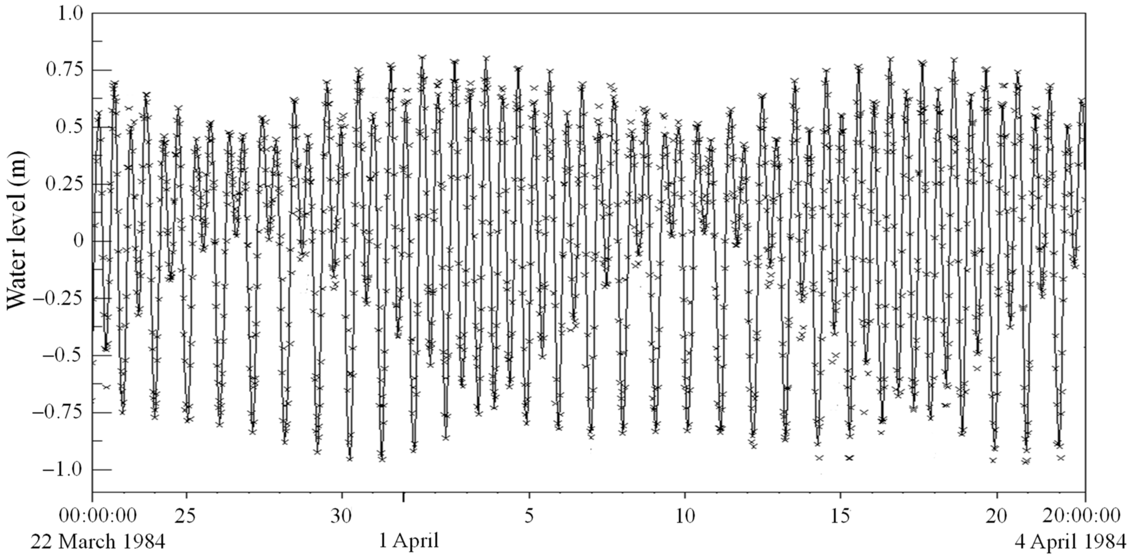
3.3. Modelled Water Levels for the Default Case of No Mariculture

Figure 6 indicates that the modeled water levels at the LS site reproduced the complete tidal processes of spring and neap tides. The time curves of the simulated water levels agree well with those of the observed water levels. For the time series of the modeled and observed water levels from 22 March to 22 April 1984, their Pearson correlation coefficient is 0.95, which indicates an excellent correlation with each other and hence the consistent tidal changes. Taking the maximal and minimal values of water levels (modeled and observed) in each of totally 61 complete tidal processes, we obtained their statistical indicators as RMSE = 0.11 m, SI = 0.18, and %Err = 15%. These values are acceptable with consideration of the following reasons. Firstly, the topography may experience changes in a certain extent between 1984 and 1999. Secondly, only the prominent hydrodynamic processes (i.e., tides) were simulated in the model, because that the purpose of this study is to evaluate the effect of the aquaculture, instead of accurately depicting physical processes of the bay. Thirdly, there are certain differences in tidal phases between the modeled and observed tides. Therefore, the default models basically reproduced actual tidal processes for the primitive bay. Next, we used the default model to set up the aquaculture model.

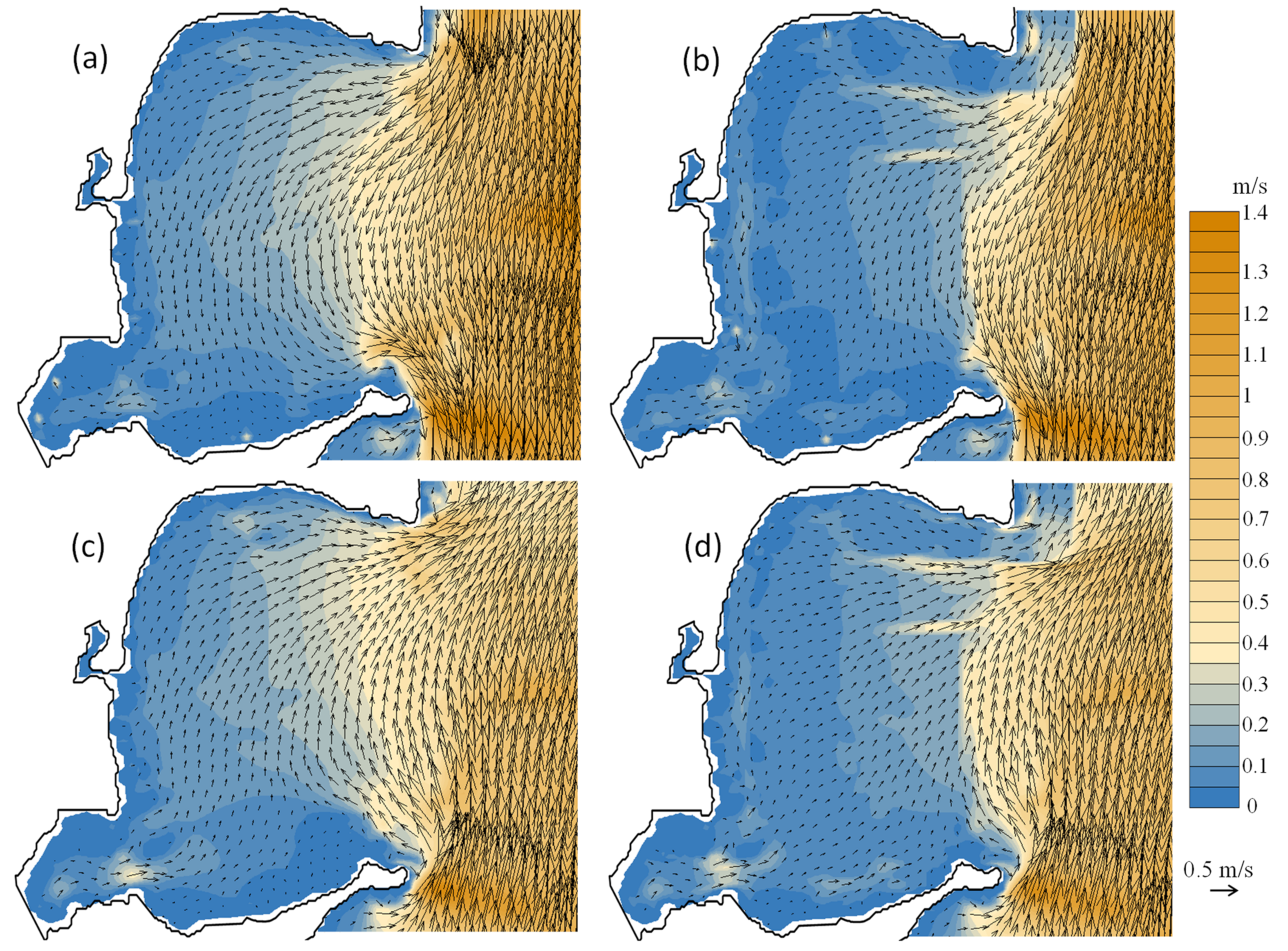
3.4. Modelled Water Currents for the Presence of Aquaculture

By numerical experiments for the approximation and calibration with the observed current velocities, we specified the appropriate energy-loss coefficients $(C_{loss-u}$ and $C_{loss-v}$) as 4.1 and 4.9 for the oyster and scallop cultures, respectively. In this circumstance, the average error of the modeled velocities at the three sites is 0.3%, and RMSE, SI, and %Err is 0.015 m/s, 0.114, and 9.9%, respectively (

Table A1. Statistical indicators in simulation errors for different numerical experiments, approaching to determine the energy-loss coefficients and ($C_{loss-u}$ and $C_{loss-v}$). O: oyster; S: scallop. Error = (p-m)/m.

${\mathit{C}}_{\mathit{l}\mathit{o}\mathit{s}\mathit{s}}$	Site	Error of Modeled Velocities at Each Layer (%)						Average Error (%)		RMSE (m/s)	SI	%Err (%)
		1	2	3	4	5	6
4.1 (O) 4.9 (S)	C1	-	29.2	30.4	13.5	−19.6	−43.8	1.9	0.3	0.015	0.113	9.8
	C2	−11.2	−4.3	18.9	1.4	0.6	−7.5	−0.4
	C3	-	0.1	−7.7	−8.4	2.9	8.6	−0.7
4.0 (O) 4.0 (S)	C1	-	30.3	31.7	14.3	−19.1	−43.7	2.7	4.9	0.018	0.137	12.1
	C2	−10.5	−3.5	19.6	1.8	0.9	−7.5	0.2
	C3	-	19.0	7.2	2.3	12.8	17.3	11.7
5.0 (O) 5.0 (S)	C1	-	25.3	26.1	11.1	−20.0	−41.5	0.2	−1.5	0.015	0.113	9.7
	C2	−14.9	−8.6	15.7	−0.3	−0.2	−6.7	−2.5
	C3	-	−0.9	−9.3	−9.6	1.8	7.6	−2.1
6.0 (O) 7.5 (S)	C1	-	21.4	22.0	7.8	−22.0	−42.2	−3.8	−7.4	0.020	0.155	13.4
	C2	−18.5	−12.8	12.2	−2.4	−1.7	−5.8	−4.8
	C3	-	−18.5	−24.2	−20.4	−8.4	−1.8	−14.7
8.0 (O) 10.0 (S)	C1	-	16.2	16.3	4.1	−23.7	−40.6	−5.5	−12.0	0.026	0.201	17.1
	C2	−23.1	−18.3	8.1	−4.6	−2.9	−4.4	−7.5
	C3	-	−29.4	−33.9	−27.7	−15.3	−8.3	−22.9
20 (O) 25 (S)	C1	-	2.9	1.3	−4.7	−26.6	−37.7	−12.9	−23.3	0.043	0.331	26.2
	C2	−36.1	−33.9	−2.3	−8.9	−4.2	−0.8	−14.4
	C3	-	−55.7	−56.9	−44.5	−31.6	−23.9	−42.5
2.7 (O) 3.3 (S)	C1	-	37.7	39.4	19.4	−17.5	−44.5	6.9	8.8	0.021	0.156	14.4
	C2	−3.6	4.6	26.2	5.7	3.1	−8.8	4.5
	C3	-	23.5	11.0	5.0	15.3	19.5	14.9
2.0 (O) 2.5 (S)	C1	-	44.1	46.2	23.7	−16.7	−44.5	10.6	15.4	0.030	0.225	20.8
	C2	2.3	11.4	32.0	9.3	5.0	−9.6	8.4
	C3	-	41.7	25.9	15.6	24.8	27.7	27.1
0.8 (O) 1.0 (S)	C1	-	66.5	70.2	39.2	−11.3	−45.4	23.9	38.2	0.067	0.512	44.3
	C2	21.7	33.4	50.7	20.0	9.9	−11.5	20.7
	C3	-	106.8	79.1	52.5	57.9	53.9	70.0

in Appendix A). Table A1 also presents the statistical indicators of model errors in some other numerical simulations taking various coefficients, and indicates the approaching process to determine the reasonable energy-loss coefficients.

Figure 7 presents the modeled current velocities in the six layers at the three sites for the presence of oyster and scallop cultures in the bay. The modeled velocities were generally consistent with the observed values in the quantity and vertical profiles. In the upper and middle layers, where aquaculture existed, the velocities were lower than those in the lower layer. At C1, where the oyster-culture facilities were arranged in the second and third layers (~1.6–3.0 m) of the model, the velocities in the two layers were low. At C2, the minimum velocities were in the second layer where oysters were cultured, and the largest velocities were in the fifth layer. At C3, the culture layers were set as the second and third layers in the model, where the scallop facilities produced the lowest velocities. According to both the modeled results and the observations at C2 and C3, the velocities in the culture layer were lower than those in the bottom layer, which indicates that the friction of the culture facilities surpassed the bottom friction. At C1, the reduction in the velocities in the culture layer was modeled as ~21% (compared with the fifth layer), which is a relatively large deviation from the observation. Because the observed data at this site are somewhat discontinuous (indicated by Figure 5a), we focused on the results at the other oyster site (C2), where the reduction was ~34%; the vertical distribution of the modeled currents agrees well with that of the observed currents (Figure 7e). At Site C3, the modeled reduction rate was up to 55%, and the modeled vertical distribution of the currents tallies with that of the observed (Figure 7f).

Although kelp was not cultured in the bay during the field investigation, we also modeled its impact. Considering that the suspension of the kelp was denser than those of the bivalves, we specified the energy-loss coefficient for kelp as 6.0. In this condition (without observations for calibration), according to the model, the velocity in the culture layer was reduced by ~60% (compared with the maximum velocities in the lower layers). This value is within the range of ~50–75%, as was observed in 2006 in this bay [12].

In short, by adding the energy-loss coefficients in the culture layer(s), the model reproduced the features of the water currents, and particularly the vertical regimes of the current velocities in the aquaculture areas.

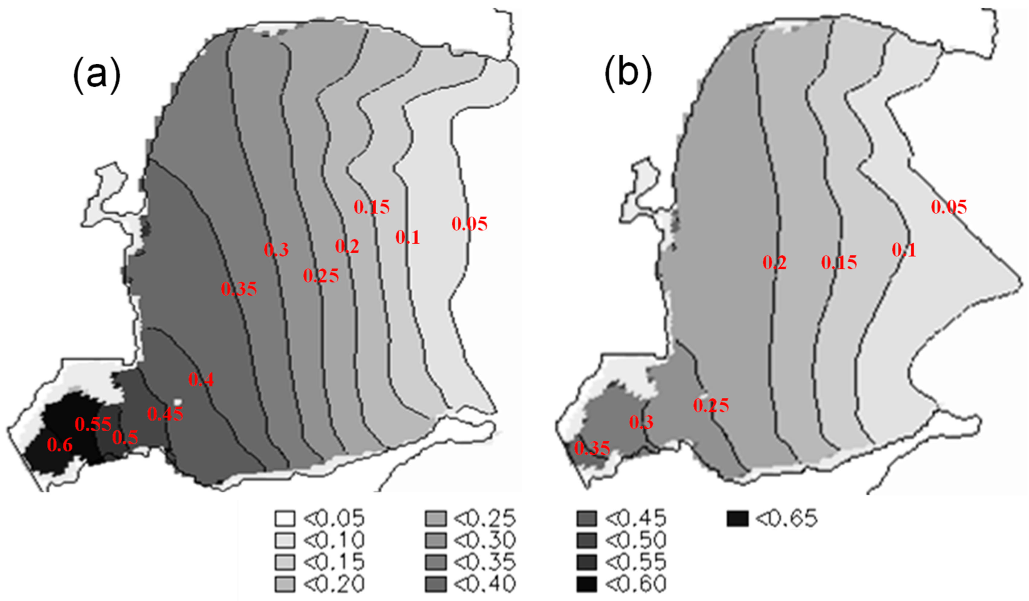
3.5. Effects of Aquaculture on Water Exchange

Because of the existence of large-scale and high-density aquaculture, the water current velocities were significantly reduced, and the hydrodynamic patterns were not identical to those of the primitive bay. Figure 8 shows depth-averaged tidal currents in the presence and absence of bivalve cultures. When the tide is rising, the water flows into the bay via the northern mouth, and out of the bay at the southern mouth, and it flows in the opposite direction when the tide is ebbing. At the northern mouth, the scallop facilities reduced the inflows (Figure 8b) and outflows (Figure 8d). In the inner area where scallops and oysters were cultured, the velocities were significantly reduced. In the presence of bivalve cultures, the velocities were less than 0.1 m/s in more than 50% of the inner bay. Thus, the water exchange in the bay was indeed affected. According to the model results, regardless of the presence of aquaculture, the half-exchange period for the bay is ~8 d, whereas it is ~12 d with the presence of bivalve cultures (configured as Figure 1b). The period is ~16 d for the configuration with all three cultured species. Compared with the absence of aquaculture, the presences of bivalve (oyster and scallop) cultures and kelp and bivalve cultures in the bay caused 33% and 50% decreases in the water-exchange ability, respectively. As a result, the aquaculture facilities impeded the flow of substances into or out of the bay. We reaffirmed this by comparing the modeled concentrations of the conceptual substance after 40 d of diffusion between the case with bivalve cultures and the case with no cultures (Figure 9). In the middle zone of the bay, the average concentration is ~0.25 for the former case, and 0.15 for the latter. The impedance is more significant in the southwestern zone, where the concentration in the presence of bivalve cultures (~0.55) is ~83% higher than that in the absence of cultures in the bay (~0.3).

4. Discussion

This study conducted by means of a field survey and a numerical model highlighted that aquaculture activities have significant influences on water currents and substance exchange in culture areas. The velocities in the culture layer were evidently attenuated by suspension culture. We set up a model that uses the drag coefficient C_z to define the momentum loss due to bottom friction in order to correctly reproduce water current fields in Sungo Bay. In Equation (1), the momentum sink of the bottom layer caused by bottom friction in the x direction is [35]:

$$\gamma \frac{\partial u}{\partial z}=C_z{\left(u^2+u^2\right)}^{1/2}u,\mathrm{when} z \to \mathrm{the} \mathrm{bottom} \mathrm{depth}$$

(10)

Similarly, we defined the momentum loss in the culture layer that is caused by aquaculture facilities, and obtained the following expression from Equation (1) and expression (10):

$$\gamma \frac{\partial u}{\partial z}=C_{ax}{\left(u^2+u^2\right)}^{1/2}u=\Delta D{M}_x$$

(11)

where $C_{ax}$ is the drag coefficient of the facilities, and $\Delta D$ is the thickness of a vertical grid cell where culture exists. Therefore, the drag coefficient in the x direction is:

$$C_{ax}=-\frac{\Delta D}{\Delta x}{C}_{loss-u}$$

(12)

By using Equation (12), we can specify the drag coefficient for high-density aquaculture areas for other hydrodynamic models, such as the Princeton Ocean Model [35]. For an example, if $\Delta D=1 \mathrm{m}$ and $\Delta x$ = 100 m, then $C_{ax}$ = 0.041 for a vertical grid cell where oysters are cultured. Nevertheless, the drag coefficient is related to the culture species, spacing of facilities, culture scale, and culture density. Therefore, the coefficient may need to be adjusted to suit different bays by numerical experiments. We also need to study the drag coefficients or energy-loss coefficients in different directions, considering the layout orientation of culture facilities. In addition, the coefficient could be quantified by physical experiments in the laboratory current tank [19].

Numerical simulations indicated that culture facilities retarded the substance-exchange process contributing to cause adverse effects on ecology, water quality, and aquaculture itself. Therefore, disregarding impacts of the facilities will inevitably result in a substantial decrease in the water-renewal period, and thus an underestimation of the pollutant dilution capacity of the water body.

5. Conclusions

According to field observations in Sungo Bay, aquaculture activities have a significant influence on the water currents in culture areas. The current velocities in the culture layer were evidently attenuated by the suspension culture. Compared with the layers without culture, the maximum reductions in the current velocities of the oyster-culture layer were ~68% and ~43% at two sites, and up to ~65% for the scallop-culture layer. According to the modeled results, the velocities in a kelp-culture layer were reduced by ~60% compared with those in the lower layer.

We constructed the model to reproduce the water currents in the culture waters of Sungo Bay by adding a porous structure that causes the momentum energy loss of water in the culture layer. By numerical simulation and calibration, the appropriate energy-loss coefficients for the suspended culture facilities were specified as 4.1, 4.9 and 6.0 for kelp, scallop, and oyster, respectively. The modeled results are essentially consistent with the observations. The method and results in this paper provide a reference for studies on other aquaculture bays and for other culture species.

The aquaculture slowed down the substance-exchange process. Without culture, the half-exchange period for Sungo Bay was modeled as ~8 d, whereas it was ~12 d in the presence of bivalve cultures, and ~16 d in the presence of kelp and bivalve cultures. Compared with the primitive situation, the former and latter configurations of the aquaculture resulted in 33% and 50% decreases in the water-exchange ability of the bay, respectively. In the future, we should further study the effects of aquaculture on environmental ecology by coupling physical-biochemical processes.

References

1. CIMA (Chinese Institute for Marine Affairs). China’s Ocean Development Report; Ocean Press: Beijing, China, 2013; p. 403.
2. Jiang, Y.; Mu, Y.; Yao, L. A study on the contributions of inputs factors to the seawater mariculture output in China—Analysis based on the panel data by coastal province. Mar. Econ. 2013, 3, 32–37. [Google Scholar]
3. FAO (Food and Agriculture Organization). The State of World Fisheries and Aquaculture 2018-Meeting the Sustainable Development Goals; Food and Agriculture Organization of the United Nations: Rome, Italy, 2018. [Google Scholar]
4. Ferreira, J.G.; Andersson, H.C.; Corner, R.A.; Desmit, X.; Fang, Q.; Goede, E.D.; Groom, S.B.; Gu, H.; Gustafsson, B.G.; Hawkins, A.J.S.; et al. SPEAR: Sustainable Options for People Catchment and Aquatic Resources; Institute for Marine Research: Lisbon, Portugal, 2008; p. 180. [Google Scholar]
5. Yang, Y.; Li, C.; Nie, X.; Tang, D.; Chuang, I. Development of mariculture and its impacts in Chinese coastal waters. Rev. Fish Biol. Fish. 2004, 14, 1–10. [Google Scholar]
6. Ma, C.; Zhang, X.; Chen, W.; Zhang, G.; Duan, H.; Ju, M.; Li, H.; Yang, Z. China’s special marine protected area policy: Trade-off between economic development and marine conservation. Ocean. Coast. Manag. 2013, 76, 1–11. [Google Scholar] [CrossRef]
7. Zhang, Z.; Huang, H.; Liu, Y.; Bi, H.; Yan, L. Numerical study of hydrodynamic conditions and sedimentary environments of the suspended kelp aquaculture area in Heini Bay. Estuar. Coast. Shelf Sci. 2020, 232, 106492. [Google Scholar] [CrossRef]
8. Newell, C.R.; Richardson, J. The effects of ambient and aquaculture structure hydrodynamics on the food supply and demand of mussel rafts. J. Shellfish. Res. 2014, 33, 257–272. [Google Scholar] [CrossRef]
9. Bacher, C.; Grant, J.; Hawkins, A.J.S.; Fang, J.; Zhu, M.; Besnard, M. Modelling the effect of food depletion on scallop growth in Sungo Bay (China). Aquat. Living Resour. 2003, 16, 10–24. [Google Scholar] [CrossRef]
10. Duate, P.; Meneses, R.; Hawkins, A.J.S.; Zhu, M.; Fang, J.; Grant, J. Mathematical modeling to assess the carrying capacity for multi-species culture within coastal waters. Ecol. Model 2003, 168, 109–143. [Google Scholar]
11. Nunes, J.P.; Ferreira, J.G.; Lencart-Silva, J.; Zhang, X.; Zhu, M.; Fang, J. A model for sustainable management of shellfish polyculture in coastal bays. Mariculture 2003, 219, 257–277. [Google Scholar] [CrossRef]
12. Fan, X.; Wei, H.; Yuan, Y.; Zhao, L. The features of vertical structures of tidal current in a typical coastal mariculture area of China. Period. Ocean Univ. China 2009, 39, 181–186. [Google Scholar]
13. Zeng, D.; Huang, D.; Qiao, X.; He, Y.; Zhang, T. Effect of suspended kelp culture on water exchange as estimated by in situ current measurement in Sanggou Bay, China. J. Mar. Syst. 2015, 149, 14–24. [Google Scholar] [CrossRef]
14. Zhu, M.; Zhang, X.; Li, R.; Chen, S. Impacts of shellfish culture on the coastal ecosystem. J. Ocean. Univ. Qingdao 2000, 30, 53–57. [Google Scholar]
15. Fang, J.; Strand, O.; Liang, X.; Zhang, J. Carrying capacity and optimizing measures for mariculture in Sungo Bay. Mar. Fish. Res. 2001, 22, 57–63. [Google Scholar]
16. Plew, D.R.; Spigel, R.H.; Stevens, C.L.; Nokes, R.I.; Davidson, M.J. Stratified flow interactions with a suspended canopy. Environ. Fluid Mech. 2006, 6, 519–539. [Google Scholar] [CrossRef]
17. Pilditch, C.A.; Grant, J.; Bryan, K.R. Seston supply to sea scallops (Placopecten magellanicus) in suspended culture. Can. J. Fish. Aquat. Sci. 2001, 58, 241–253. [Google Scholar] [CrossRef]
18. Zhang, X.; Zhu, M.; Li, R.; Wang, Z. Simultaneous and consecutive multi-parameter monitoring of shellfish culture environment. Adv. Mar. Sci. 2004, 22, 340–346. [Google Scholar]
19. Wang, T.; Khangaonkar, T.; Long, W.; Gill, G. Development of a Kelp-Type structure module in a coastal ocean model to assess the hydrodynamic impact of seawater uranium extraction technology. J. Mar. Sci. Eng. 2014, 2, 81–92. [Google Scholar] [CrossRef]
20. Grant, J.; Bacher, C. A numerical model of flow modification induced by suspended mariculture in a Chinese bay. Can. J. Fish. Aquat. Sci. 2001, 58, 1003–1011. [Google Scholar] [CrossRef]
21. Liu, X.; Pu, X.; Luo, D.; Lu, J.; Liu, Z. Model assessment of nutrient removal via planting Sesuvium portulacastrum in floating beds in eutrophic marine waters: The case of aquaculture areas of Dongshan Bay. Acta Oceanol. Sin. 2019, 38, 91–100. [Google Scholar] [CrossRef]
22. Grant, J.; Stenton-Dozey, J.; Monteiro, P.; Pitcher, G.; Heasman, K. Shellfish culture in the Benguela system: A carbon budget of Saldanha Bay for raft culture of Mytilus galloprovincialis. J. Shellfish Res. 1998, 17, 41–49. [Google Scholar]
23. O’Donncha, F.; Hartnett, M.; Nash, S. Physical and numerical investigation of the hydrodynamic implications of aquaculture farms. Aquacult. Eng. 2013, 52, 14–26. [Google Scholar] [CrossRef]
24. Shi, J.; Wei, H. Simulation of hydrodynamic structures in a semi enclosed bay with dense raft culture. Period. Ocean Univ. China 2009, 39, 1181–1187. [Google Scholar]
25. Fan, X.; Wei, H.; Yuan, Y.; Zhao, L. Vertical structure of tidal current in a typically coastal raft-culture area. Cont. Shelf Res. 2009, 29, 2345–2357. [Google Scholar] [CrossRef]
26. Rickard, G. Three-dimensional hydrodynamic modelling of tidal flows interacting with aquaculture fish cages Graham Rickard. J. Fluid. Struct. 2020, 93, 102871. [Google Scholar] [CrossRef]
27. Zhang, J.; Hansen, P.K.; Fang, J.; Wang, W.; Jiang, Z. Assessment of the local environmental impact of intensive marine shellfish and seaweed farming—application of the MOM system in the Sungo Bay, China. Aquaculture 2009, 287, 304–310. [Google Scholar] [CrossRef]
28. Deltares. Delft3D-FLOW, Simulation of Multi-Dimensional Hydrodynamic Flows and Transport Phenomena, Including Sediments, User Manual, Version 3.15; Deltares: Delft, The Netherlands, 2021; Available online: https://oss.deltares.nl/web/delft3d/manuals (accessed on 28 March 2022).
29. Bonamano, S.; Madonia, A.; Borsellino, C.; Stefann, C.; Caruso, G.; De Pasquale, F.; Piermattei, V.; Zappalt, G.; Marcelli, M. Modeling the dispersion of viable and total Escherichia coli cells in the artificial semi-enclosed bathing area of Santa Marinella (Latium, Italy). Mar. Pollut. Bull. 2015, 95, 141–154. [Google Scholar] [CrossRef]
30. Bonamano, S.; Piazzolla, D.; Scanu, S.; Mancini, E.; Madonia, A.; Piermattei, V.; Marcelli, M. Modelling approach for the evaluation of burial and erosion processes on Posidonia oceanica meadows. Estuar. Coast. Shelf Sci. 2021, 254, 107321. [Google Scholar] [CrossRef]
31. Bonamano, S.; Madonia, A.; Piazzolla, D.; de Mendoza, F.P.; Piermattei, V.; Scanu, S.; Marcelli, M. Development of a predictive tool to support environmentally sustainable management in Port Basins. Water 2017, 9, 898. [Google Scholar] [CrossRef] [Green Version]
32. Chen, G. Marine Atlas of Bohai Sea, Yellow Sea and East China Sea: Hydrology; Ocean Press: Beijing, China, 1992; pp. 429–432. [Google Scholar]
33. Li, F. Marine Hydrology Atlas of Shandong Coastal Sea; Shandong Atlas Press: Jinan, China, 1989; p. 42. [Google Scholar]
34. Luff, R.; Pohlmann, T. Calculation of water exchange times in the ICES-boxes with an eulerian dispersion model using a half-life time approach. Dtsch. Hydrogr. Z. 1996, 47, 287–299. [Google Scholar] [CrossRef]
35. Mellor, G.L. Users Guide for a Three-Dimensional, Primitive Equation, Numerical Ocean Model; Princeton University: Princeton, NJ, USA, 2004. [Google Scholar]
Figure 1. Sketch of Sungo Bay: (a) location of bay; (b) aquaculture areas for oysters, scallops, and kelp (adapted from [27] with permission from Elsevier, 2022); (c) observation locations. LS (●) is the water-level observation station; (▲) marks sites C1 and C2 (in oyster-culture zones), C3 (in scallop-culture zone), and C1n, C2n, and C3n near them (out of the culture zone) for water-current observation; round-route curves indicate observations of currents by ADCP at the bay mouth; (d) the enlarged square image (from Landsat) shows a sky view of aquaculture rafts for kelps.
Jmse 10 01151 g001
Figure 2. The (a) topography and (b) model grids of Sungo Bay. The area west of the black dashed line is the inner bay, where the water-exchange ability was computed. Red dashed lines are open boundaries.
Jmse 10 01151 g002
Figure 3. Culture methods for (a) kelps, (b) scallops, and (c) oysters; pictures for cultures of (d) kelps, (e) scallops, and (f) oysters.
Jmse 10 01151 g003
Figure 4. The current profiles observed by ADCP at the bay mouth, where little aquaculture existed. North and South represent the north and south ends (Figure 1c), respectively.
Jmse 10 01151 g004
Figure 5. Vertical profiles of current velocities observed in aquaculture areas. Time series of velocities at (a) C1, (b) C2, and (c) C3 at different depths; time-average velocities for (d) C1 vs. C1n, (e) C2 vs. C2n, and (f) C3 vs. C3n; normalized values of averaged velocities and decrease rates of velocities for (g) C1 vs. C1n, (h) C2 vs. C2n, and (i) C3 vs. C3n. Non-aquaculture sites C1n, C2n, and C3n near culture sites C1, C2, and C3, respectively. Normalized values equal to the averaged velocities divided by near-bottom velocities.
Jmse 10 01151 g005
Figure 6. Simulated (lines) and measured (markings) water levels at site (LS) without aquaculture.
Jmse 10 01151 g006
Figure 7. Vertical profiles of current velocities in aquaculture zones of Sungo Bay in the presence of bivalve cultures: simulated time series at six layers at (a) C1, (b) C2, and (c) C3 (1–6 represent the 1st–6th model layer); comparison of observed and simulated velocities (averaged within observation periods) for (d) C1, (e) C2, and (f) C3.
Jmse 10 01151 g007
Figure 8. Depth-averaged tidal currents in the bay. Tidal rising for (a) non-aquaculture and (b) bivalve cultures; tidal ebbing for (c) non-aquaculture and (d) bivalve cultures. Color bar shows the velocity magnitude. The same period and model configuration were used for simulations of no aquaculture and bivalve cultures.
Jmse 10 01151 g008
Figure 9. Concentration distributions of the conceptual substance (dimensionless) in Sungo Bay after 40 d of diffusion for cases of (a) bivalve culture and (b) no culture in the bay.
Jmse 10 01151 g009
Publisher’s Note: MDPI stays neutral with regard to jurisdictional claims in published maps and institutional affiliations.