Reliability-Based Criterion for Evaluating Explicit Approximations of Colebrook Equation

Abstract

Numerous explicit approximations of the Colebrook equation have been developed and evaluated based on two criteria: prediction accuracy and computational efficiency. This paper introduces a new evaluation criterion based on the reliability of each equation. The reliability is defined by the coefficient of variation (CV) of the explicit friction factor that is a function of the variabilities of component random variables (roughness height of the internal pipe surface and kinematic viscosity of the fluid). The coefficient of variation of the friction factor depends on its first derivative for roughness height of the inner pipe surface and kinematic viscosity of the fluid and their correlation. Seven explicit approximations were evaluated using the new reliability-based criterion. The results show that all explicit approximations are very reliable, but variations exist regarding the reliability level. The reliabilities of the seven approximations is very close for the rough-flow regime and when the CV of the viscosity is minimal. However, for the smooth-flow regime, and when the CV of the roughness is minimal, various approximations showed substantially different reliabilities. The novelty of the proposed criterion is that it addresses an evaluation dimension that complements the accuracy and efficiency criteria.

1. Introduction

The pipe friction factor f from the Darcy–Weisbach formula is given by

$$h=f·\frac{L·\rho ·V^2}{2·D}$$

(1)

where h is the head loss in meters, which can be calculated using the Colebrook equation given by [1,2,3,4]

$$\frac{1}{\sqrt{f}}=-2·{log}_{10}\left(\frac{\epsilon }{3.7·D}+\frac{2.51}{R·\sqrt{f}}\right)$$

(2)

where:

f is the dimensionless Darcy’s friction factor,

L is the length of pipe (m),

ρ is the density of the fluid (kg/m³),

V is the velocity of the fluid (m/sec),

D is the pipe diameter (m),

ε is the roughness of the inner pipe surface (m), and

R is the dimensionless Reynolds number, defined as R = V·D/ν, where

ν is the kinematic viscosity of the fluid (m²/sec).

Both the Darcy–Weisbach and the Colebrook equations are empirical. Equation (2) is based on experimentation with the flow of air through pipes with a different inner pipe roughness ranging from smooth to fully rough. Additionally, it contains unknown friction factor f on both sides of the equal sign in a form from which it cannot be extracted analytically. To overcome this inconvenience, many explicit approximations have been developed for efficient use in everyday engineering practice. Genic et al. [5] and Pracks and Brkic [6] have presented excellent reviews and evaluations of the available explicit approximations of the Colebrook equation. The evaluation criteria used for evaluating the explicit approximations were prediction accuracy and computational efficiency. The reliability of the explicit approximations has not been previously addressed in the literature.

This article introduces a new evaluation criterion based on the reliability of the explicit approximations that aims to complement the existing criteria. The new criterion was used to evaluate seven approximations of the Colebrook equation. The reliability is defined by the coefficient of variation of the explicit friction factor that is a function of the variabilities of component random variables (roughness height of the internal pipe surface and kinematic viscosity of the fluid). The coefficient of variation of the friction factor depends on its first derivative for roughness height of the inner pipe surface and kinematic viscosity of the fluid, and their correlation.

2. Materials and Methods

2.1. Explicit Approximations of Colebrook Equation

Seven explicit approximations that are evaluated through the new reliability-based criterion are by Swamee and Jain [7], Haaland [8], Mikata and Walczak [9], Biberg [10], Vatankhah [11], Praks and Brkić [6], and Lamri and Easa [12].

2.1.1. Approximation by Swamee and Jain (1976)

The approximation by Swamee and Jain [7] is given by

$$\frac{1}{\sqrt{f}}=-2\log \left(\frac{\epsilon }{3.7D}+\frac{5.74}{R^{0.9}}\right)$$

(3)

2.1.2. Haaland’s Approximation (1983)

The approximation by Haaland [8] is given by

$$\frac{1}{\sqrt{f}}\approx -1.8·{log}_{10}\left({\left(\frac{\epsilon }{3.7·D}\right)}^{1.11}+\frac{6.9}{R}\right)=-1.8·{log}_{10}\left({\zeta }_1\right)$$

(4)

2.1.3. Approximation by Mikata and Walczak (2015)

The approximation by Mikata and Walczak [9] is given by

$$\frac{1}{\sqrt{f}}\approx 0.8686·ln\left(\frac{0.458·R}{A_1-ln\left(A_1\right)}\right)={\zeta }_3$$

(5)

where A₁ is defined as

$$A_1=0.124·R·\frac{\epsilon }{D}+ln\left(0.4587·R\right)$$

(6)

2.1.4. Biberg’s Approximation (2017)

The approximation by Biberg [10] is given by

$$\frac{1}{\sqrt{f}}\approx A_2·\left[ln\left(\frac{R}{2.51·A_2}\right)+\left(\frac{1}{A_3}-A_3\right)·ln\left(A_3\right)\right]={\zeta }_4$$

(7)

where $A_2$ and $A_3$ are defined as

$$A_2=\frac{2}{ln\left(10\right)}$$

(8)

$$A_3=ln\left(\frac{R}{2.51·A_2}\right)+\frac{R}{9.287·A_2}·\frac{\epsilon }{D}$$

(9)

2.1.5. Vatankhah’s Approximation (2018)

The approximation by Vatankhah [11] is given by

$$\frac{1}{\sqrt{f}}\approx 0.8686·ln\left[\frac{0.3984·R}{{\left(0.8686·A_4\right)}^{\frac{A_4}{A_4+A_5}}}\right]={\zeta }_5$$

(10)

where $A_4$ and $A_5$ are defined as

$$A_4=0.12363·R·\frac{\epsilon }{D}+ln\left(0.3984·R\right)$$

(11)

$$A_5=1+\frac{1}{\frac{1+A_4}{0.5·ln\left(0.8686·A_4\right)}-\frac{1+4·A_4}{3·\left(1+A_4\right)}}$$

(12)

2.1.6. Approximation by Praks and Brkić (2020)

The approximation by Praks and Brkić [6] is given by

$$\frac{1}{\sqrt{f}}\approx 0.8686·\left[A_8-A_9+\frac{A_9}{A_6-0.5564·A_9+1.207}\right]=0.8686·\left[A_8-A_9+\frac{A_9}{{\zeta }_6}\right]$$

(13)

where $A_6$, $A_7$, $A_8$, and $A_9$ are defined as

$$A_6=A_7+A_8$$

(14)

$$A_7=\frac{R}{8.0884}·\frac{\epsilon }{D}$$

(15)

$$A_8=ln\left(R\right)-0.7794$$

(16)

$$A_9=ln\left(A_6\right)$$

(17)

2.1.7. Approximation by Lamri and Easa (2022)

The approximation by Lamri [13] and Lamri and Easa [12] is given by

$$\frac{1}{\sqrt{f}}\approx A_{10}+2·{log}_{10}\left(A_{11}\right)·\left(-1+\frac{0.862}{A_{11}}·\left[1+\frac{1}{A_{11}}·{log}_{10}\left(\frac{A_{11}}{e^2}\right)\right]\right)$$

(18)

where $A_{10}$ and $A_{11}$ are defined as

$$A_{10}=2·{log}_{10}\left(\frac{R}{2.51}\right)$$

(19)

$$A_{11}=\frac{R}{9.287}·\frac{\epsilon }{D}+A_{10}$$

(20)

Brkic and Stajic [14] affirmed that Equation (18) is the most efficient available approximation of the Colebrook equation.

2.2. Proposed Reliability Criterion

2.2.1. Reliability Definition

The friction factor of the Colebrook approximations is a nonlinear function of the random variables ν and ε, and therefore f is also a random variable. To derive the reliability of the friction factor f, it is necessary to linearize its solution. In general, let Y be a nonlinear function of several random variables, X_i, I = 1, 2, …, n, where n is the number of random variables. That is, Y = F(X₁, X₂, …, X_n). Then, using the Taylor series, the expected value and variance of Y, E[Y] and var[Y], are given, respectively, by [15,16].

$$E\left[Y\right] \cong \mathrm{F}(\mu x_1,\mu x_1,\dots ,\mu x_n)$$

(21)

$$var\left[Y\right]\cong {{\displaystyle \sum }}_{i=1}^n{\left(\frac{\partial F}{\partial X_i}\right)}^2{\sigma }_{Xi}^2+{{\displaystyle \sum }}_{i }^n{{\displaystyle \sum }}_j^n\left(\frac{\partial F}{\partial X_i}\right)\left(\frac{\partial F}{\partial X_j}\right)cov\left[X_i,X_j\right]$$

(22)

where μ_Xi is the mean value of the random variable X_i, σ_Xi is the standard deviation (SD) of the random variable X_i, and cov[X_i, X_j] is the covariance of the random variables X_i and X_j. The covariance between two random variables is given by cov[X_i, X_j] = ρ_Xi,Xj σ_Xi σ_Xj, where ρ_Xi,Xj is the correlation coefficient between X_i and X_j. The coefficient of variation of Y, which is a dimensionless measure of reliability, is given by

$$C{V}_Y=\frac{\sqrt{var\left[Y\right]}}{E\left[Y\right]}$$

(23)

where CV_Y is the coefficient of variation of the random variable Y and µ_Y is the mean of the random variable Y. Similarly, CV_xi = σ_Xi/µ_Xi.

The coefficient of variation has been used in engineering applications to determine the reliability of a random variable. The smaller the CV value, the more reliable the random variable is.

The definition of reliability is graphically presented in Figure 1.

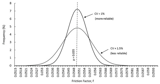
Figure 1. Definition of reliability.

2.2.2. First Derivatives of Friction Factor f

Since the friction factor f of the Colebrook equation is a nonlinear function of the random variables v and ε, the mean and standard deviation of f are given by

$$\begin{array}{c}E\left[f\right]\cong F\left({\mu }_v, {\mu }_{\epsilon }\right)\\ var\left[f\right]\cong {\left(\frac{\partial f}{\partial v}\right)}^2{\sigma }_v^2+{\left(\frac{\partial f}{\partial \epsilon }\right)}^2{\sigma }_{\epsilon }^2+\left(\frac{\partial f}{\partial v}\right)\left(\frac{\partial f}{\partial \epsilon }\right)cov\left[v,\epsilon \right]\\ \begin{array}{c}cov\left[v,\epsilon \right]={\rho }_{v,\epsilon }{\sigma }_v{\sigma }_{\epsilon }\\ C{V}_f=\frac{\sqrt{var\left[f\right]}}{E\left[f\right]}\end{array}\end{array}\}$$

(24)

The first derivatives of f for v and ε are needed for calculating the variance and expected value of f, and the coefficient of variation of f. These derivatives are presented next for the seven explicit approximations of the Colebrook equation, respectively, presented in Section 2.1.

-

Approximation by Swamee and Jain:

$$\begin{array}{c}\frac{df}{d\epsilon }=\frac{4}{3.7·D·ln\left(10\right)}·{\left[-2·{log}_{10}\left({\zeta }_2\right)\right]}^{-3}·{\left[ln\left({\zeta }_2\right)\right]}^{-1}\\ \begin{array}{c}\frac{df}{d\nu }=\frac{5.934}{{\nu }^{0.1}·ln\left(10\right)}·{\left(\frac{\pi ·D}{Q}\right)}^{0.9}·{\left[-2·{log}_{10}\left({\zeta }_2\right)\right]}^{-3}·{\left[ln\left({\zeta }_2\right)\right]}^{-1}\\ {\zeta }_2=\frac{\epsilon }{3.7·D}+\frac{5.74}{R^{0.9}}\end{array}\end{array}\}$$

(25)

-

Haaland’s approximation:

$$\begin{array}{c}\frac{df}{d\epsilon }=\frac{3.6}{ln\left(10\right)}·{\left[-1.8·{log}_{10}\left({\zeta }_1\right)\right]}^{-3}·\left(\frac{1.11·{\epsilon }^{0.11}}{{\left(3.7·D\right)}^{1.11}}\right)·{\left[{\zeta }_1\right]}^{-1}\\ \begin{array}{c}\frac{df}{d\nu }=\frac{3.6}{ln\left(10\right)}·{\left[-1.8·{log}_{10}\left({\zeta }_1\right)\right]}^{-3}·\left(\frac{6.9·\pi ·D}{4·Q}\right)·{\left[{\zeta }_1\right]}^{-1}\\ {\zeta }_1={\left(\frac{\epsilon }{3.7·D}\right)}^{1.11}+\frac{6.9}{R}\end{array}\end{array}\}$$

(26)

-

Approximation by Mikata and Walczak:

$$\begin{array}{c}\frac{df}{d\epsilon }=-2·0.8686·{\left[{\zeta }_3\right]}^{-3}·\left(\frac{-0.124·R}{D·\left(A_1-ln\left(A_1\right)\right)}\right)·\left(1-\frac{1}{A_1}\right)\\ \begin{array}{c}\frac{df}{d\nu }=-2·0.8686·{\left[{\zeta }_3\right]}^{-3}·\left[\left(\frac{-4·Q}{R·\pi ·D·{\nu }^2}\right)-{\left(A_1-ln\left(A_1\right)\right)}^{-1}·\left(\frac{d{A}_1}{d\nu }\right)\left(1-\frac{1}{A_1}\right)\right]\\ \begin{array}{c}{\zeta }_3=0.8686·ln\left(\frac{0.458·R}{A_1-ln\left(A_1\right)}\right)\\ \frac{d{A}_1}{d\nu }=\frac{-0.124·4·Q·\epsilon }{\pi ·D^2·{\nu }^2}-\frac{1}{\nu }\end{array}\end{array}\end{array}\}$$

(27)

-

Biberg’s approximation:

$$\begin{array}{c}\frac{df}{d\epsilon }=-2·A_2·{\left[{\zeta }_5\right]}^{-3}·\left[\left(\frac{1}{A_3}-1\right)·\left(\frac{R}{9.287·z·A_3·D}\right)-ln\left(A_3\right)·\left(\frac{R}{9.287·z·A_3{}^2·D}\right)\right]\\ \begin{array}{c}\frac{df}{d\nu }=-2·A_2·{\left[{\zeta }_5\right]}^{-3}·\left[\frac{-1}{\nu }+\frac{1}{A_3}·\frac{d{A}_3}{d\nu }\left(\frac{1}{A_3}-1\right)-\frac{ln\left(A_3\right)}{A_3{}^2}·\frac{d{A}_3}{d\nu }\right]\\ {\zeta }_4=A_2·\left(ln\left(\frac{R}{2.51·A_2}\right)+\left(\frac{1}{A_3}-1\right)·ln\left(A_3\right)\right)\end{array}\end{array}\}$$

(28)

-

Vatankhah’s approximation:

$$\begin{array}{c}\frac{df}{d\epsilon }=2·{\left(0.8686\right)}^2·{\left[{\zeta }_5\right]}^{-3}·\left(\frac{0.1236·A_4·R}{D·\left(A_4+A_5\right)·\left(0.8686·A_4\right)}\right)\\ \begin{array}{c}\frac{df}{d\nu }=2·0.8686·{\left[{\zeta }_5\right]}^{-3}·\left[\frac{1}{\nu }-\left(1-\frac{1}{\nu ·\left(A_4+A_5\right)}\right)\right]\\ {\zeta }_5=0.8686·\ln \left(\frac{0.3984·R}{{\left(0.8686·A_4\right)}^{\frac{A_4}{A_4+A_5}}}\right)\end{array}\end{array}\}$$

(29)

-

Approximation by Praks and Brkić:

$$\begin{array}{c}\frac{df}{d\epsilon }=-2·0.8686·{[0.8686·[A_8-A_9+\frac{A_9}{{\zeta }_6}\left]\right]}^{-3}·[-\frac{d{A}_6}{d_{\epsilon }}·\frac{1}{A_6}+\frac{\frac{d{A}_6}{d_{\epsilon }}·\frac{1}{A_6}·{\zeta }_6-A_9(\frac{d{A}_6}{d_{\epsilon }}-0.5564·\frac{d{A}_6}{d_{\epsilon }}·\frac{1}{A_6})}{{A_6}^2}]\\ \frac{df}{d\nu }=-2·0.8686·{[0.8686·[A_8-A_9+\frac{A_9}{{\zeta }_6}\left]\right]}^{-3}·[\frac{-1}{\nu }-\frac{d{A}_6}{d_{\nu }}·\frac{1}{A_6}+\frac{\frac{d{A}_6}{d_{\epsilon }}·\frac{1}{A_6}·{\zeta }_6-A_9(\frac{d{A}_6}{d_{\epsilon }}-0.5564·\frac{d{A}_6}{d_{\epsilon }}·\frac{1}{A_6})}{{A_6}^2}]\\ {\zeta }_6=A_6-0.5564·A_9+1.207\\ \frac{d{A}_6}{d_{\nu }}=\frac{-4·Q·\epsilon }{8.0884·\pi D^2·{\nu }^2}-\frac{1}{\nu }\end{array}\}$$

(30)

-

Approximation by Lamri and Easa:

$$\begin{array}{c}\frac{df}{d\epsilon }=-2·{\left[{\zeta }_7\right]}^{-3}·\left[\right(\frac{0.8645}{A_{11}}-1)·(\frac{2·R}{9.287·D·A_{11}ln\left(10\right)})+2·{log}_{10}(A_{11})·(\frac{-0.8645·R}{9.287·D·{A_{11}}^2}\left)\right]\\ \frac{df}{d\nu }=-2·{\left[{\zeta }_7\right]}^{-3}·\left[\right(\frac{-2}{\nu ·ln\left(10\right)})+(\frac{0.8645}{A_{11}}-1)·(\frac{d{A}_{11}}{d_{\nu }})+{log}_{10}(A_{11})·(\frac{d{A}_{11}}{d_{\nu }}\left)\right]\\ {\zeta }_7=A_{10}+2·{log}_{10}\left(A_{11}\right)·(\frac{0.8645}{A_{11}}-1)\\ \frac{d{A}_{11}}{d_{\nu }}=\frac{-4·Q·\epsilon }{8.0884·\pi D^2·{\nu }^2}-\frac{2}{\nu ·ln\left(10\right)}\end{array}\}$$

(31)

2.2.3. Verification

To verify the developed derivatives, the mean and standard deviation of f of the analytical formulas were compared with those of the Monte Carlo simulation. Given the means of ν and ε and the assumed values of CV, the expected value and standard deviation of f were obtained. For simplicity, ν and ε were assumed to be uncorrelated (${\rho }_{v,\epsilon }$ = 0). The simulation involved generating 20,000 random values of the four random variables ν and ε, assuming their probability distributions to be normal. The generated random values of the two variables were then substituted in the respective equation of f of the corresponding approximation, resulting in 20,000 values of f that were used to establish a frequency histogram.

The analytical and MC simulation results of all explicit approximations were very close. This verifies the developed first derivatives. For example, a comparison of the simulation and mathematical results of the approximation by Lamri and Easa [12] is shown in Figure 2. The hollow columns represent a normal distribution with the respective mean and SD of the mathematical solution. The solid columns represent the frequency distribution based on simulation. It is noted that the means and standard deviations of the mathematical formula and simulation are very close, and the distribution of f is also close to normal.

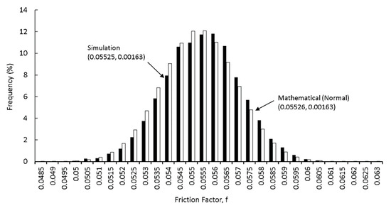
Figure 2. Comparison of the frequency distributions of analytical and simulation for the approximation by Lamri and Easa [12].

3. Results

3.1. Reliability-Based Ranking of Various Approximations

The reliability of various approximations was evaluated for the following four cases:

Case 1: Coefficient of variation of ε is zero (CV_ε = 0, CV_ν = 30%).

Case 2: Coefficient of variation of v is zero (CV_ε = 30%, CV_ν = 0).

Case 3: Smooth-flow regime (ε = 0, ν = 1 × 10⁻⁶).

Case 4: Rough-flow regime (ε = 0.001, ν = 2 × 10⁻⁹).

The reliabilities of some methods were very close in the preceding cases. To fairly reflect the ranking of various approximations, the minimum coefficient of variation of f, min CV_f, was calculated for each case, and the rankings of the approximations were determined as follows:

Rank 1: min CV_f ≤ CV_f < 1.1 min CV_f.

Rank 2: 1.1 min CV_f ≤ CV_f < 1.2 min CV_f.

Rank 3: 1.2 min CV_f ≤ CV_f.

Thus, an approximation is assigned Rank 1 if its CV_f lies within 110% of min CV_f and Rank 2 if its CV_f lies within 110% and 120% of min CV_f. If CV_f is equal to or greater than 120% of min CV_f, the approximation is assigned Rank 3.

The ranking results are shown in Table 1. For each case, the minimum and maximum CV_f are shown. For example, for Case 3, min CV_f = 4.438 and max CV_f = 5.449. The 110% and 120% thresholds are 4.438 and 4.881, respectively. The approximation of Swamee and Jain is assigned Rank 1 because their CV_f is the minimum. The CV_f of all other approximations are greater than 4.881 and therefore were assigned Rank 3.

Table 1. Rankings of various approximations based on the reliability criterion.

Approximation	CV Level		Flow regime
	Case 1: CVε = 0	Case 2: CVv = 0	Case 3: Smooth 1	Case 4: Rough 2
	CVν = 30% (CVf = 0.210–0.415)	CVε = 30% (CVf = 8.172–8.354)	ε = 0, ν = 1 × 10−6 (CVf = 4.438–5.449)	ε = 0.001, ν = 2 × 10−9 (CVf = 5.701–5.706)
Swamee and Jain	3	1	1	1
Haaland	1	1	3	1
Mikata and Walczak	2	1	3	1
Biberg	2	1	3	1
Vatankhah	3	1	3	1
Praks and Brkic	2	1	3	1
Lamri and Easa	2	1	3	1

¹ CV_ε = 0, CV_ν = 30%. ² CV_ε = 20%, CV_ν = 30%.

Thus, for Case 1, Haaland’s approximation is the most reliable (Rank 1), while the approximations by Swamee and Jain and Vatankhah are the least reliable (Rank 3). The other approximations have Rank 2). For Case 3, the approximation by Swamee and Jain substantially outperforms the other approximations. For Cases 2 and 4, all approximations are assigned Rank 1 because their reliabilities are within 110% of the min CV_f (8.990 and 6.627, respectively).

3.2. Sensitivity Analysis

The variation of the reliability of various approximations was examined as v or ε varies. The variation CV_f of various approximations as the roughness varies is shown in Figure 3 for CV_ε = 0, CV_ν = 30%, and ν = 1 × 10⁻⁶. The log(ε) varied from −1.5 to −5. As noted, as the roughness decreases to about −3, CV_f of all approximations is almost the same. As the roughness decreases further, CV_f of Swamee and Jain’s approximation becomes the best, and all other approximations exhibit substantially larger values, consistent with Case 3 of Table 1.

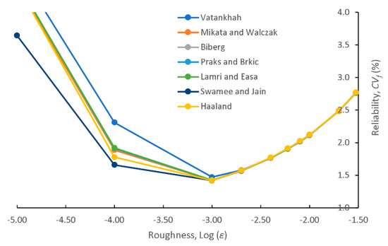
Figure 3. Variation of the reliability of various approximations as roughness varies (ν = 1 × 10⁻⁶, CV_ε = 0, CV_ν = 30%).

The variation CV_f of various approximations as the viscosity varies is shown in Figure 4 for the smooth-flow regime (ε = 0). This is similar to Case 3 of Table 1, except that v varies. As noted, Swamee and Jain’s approximation exhibits the best reliability for the entire range of v. The reliability of the other approximations is almost the same. However, for larger viscosity, Haaland’s approximation shows the least reliability.

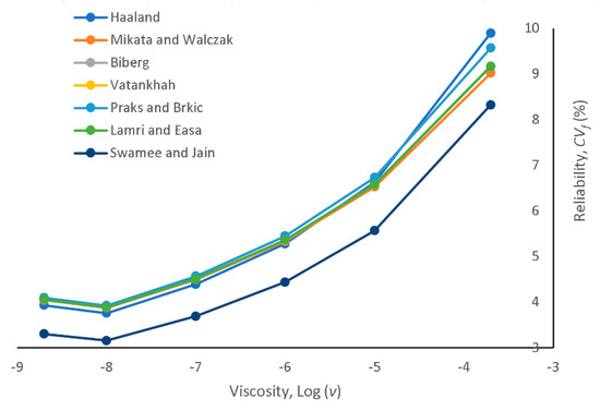
Figure 4. Variation of the reliability of various approximations as viscosity varies for the smooth-flow regime (ε = 0).

4. Conclusions

This article has introduced a new reliability-based criterion for evaluating the performance of the explicit approximations of the Colebrook equation. The proposed criterion addresses a performance dimension that complements the existing prediction accuracy and computational efficiency criteria. The criterion was used to evaluate the performance of seven explicit approximations.

The new criterion is defined by the coefficient of variation of the explicit friction factor. The CV_f of the friction factor is calculated using the variabilities of the two random parameters: roughness height of the internal pipe surface and kinematic viscosity of the fluid. The coefficient of variation of the friction factor depends on its first derivatives for these two parameters and their correlation.

The results show that all explicit approximations are very reliable, but variations exist regarding the reliability level. The reliabilities of the seven approximations were close for the rough-flow regime and when the CV of viscosity is minimal (all approximations have Rank 1). For the smooth-flow regime, Swamee and Jain’s approximation showed the largest reliability (Rank 1), while the other approximations were close (Rank 3). When the CV of the roughness is minimal, Haaland’s approximation showed the largest reliability (Rank 1), followed by the approximations by Mikata and Walczak, Biberg, Praks and Brkic, and Lamri and Easa (Rank 2). In contrast, Vatankhah’s approximation showed the least reliability (Rank 3). The sensitivity analysis shows that, for CV_ε = 0, the performance of various explicit approximations is the same for large ε, and the performance varies as ε decreases. In addition, for the smooth-flow regime (ε = 0), the relative performance remains almost the same for the entire range of v.

References

- Colebrook, C.F.; White, C.M. Experiments with Fluid Friction in Roughened Pipes. Proc. R. Soc. London. Ser. A—Math. Phys. Sci. 1937, 161, 367–381. [Google Scholar] [CrossRef]
- Colebrook, C.F. Turbulent Flow in Pipe with Particular Reference to the Transition Region Between the Smooth and Rough Pipe Laws. J. Inst. Civ. Eng. 1939, 11, 133–156. [Google Scholar] [CrossRef]
- Darcy, H. Recherches Expérimentales Relative au Mouvement de l’eau dans les Tuyaux; Mallet-Bachelier: Paris, France, 1857. (In French) [Google Scholar]
- Weisbach, J. Lehrbuch der Ingenieur-und Maschinen. Mechanik 1845, 1, 434. [Google Scholar]
- Genić, S.; Aranđelović, I.; Kolendić, P.; Jarić, M.; Budimir, N.; Genić, V. A Review of Explicit Approximations of Colebrook Equation. FME Trans. 2011, 39, 67–71. Available online: https://scindeks.ceon.rs/article.aspx?artid=1451-20921102067G (accessed on 8 June 2022).
- Praks, P.; Brkić, D. Review of New Flow Friction Equations: Constructing Colebrook’s Explicit Correlations Accurately. Rev. Int. De Métodos Numéricos Para Cálculo Y Diseñoen Ing. 2020, 36, 41. [Google Scholar] [CrossRef]
- Swamee, P.K.; Jain, A.K. Explicit Equations for Pipe Flow Problems. J. Hydraul. Eng. 1976, 102, 657–664. [Google Scholar] [CrossRef]
- Haaland, S.E. Simple Explicit Formulas for the Friction Factor in Turbulent Pipe Flow. ASME J. Fluids Eng. 1983, 105, 89–90. [Google Scholar] [CrossRef]
- Mikata, Y.; Walczak, S. Exact Analytical Solutions of the Colebrook White Equation. J. Hydraul. Eng. 2016, 142, 04015050. [Google Scholar] [CrossRef]
- Biberg, D. Fast and Accurate Approximations for the Colebrook Equation. J. Fluids Eng. 2017, 139, 031401. [Google Scholar] [CrossRef]
- Vatankhah, A. Approximate Analytical Solution for the Colebrook Equation. J. Hydraul. Eng. 2018, 144, 06018007. [Google Scholar] [CrossRef]
- Lamri, A.; Easa, S.M. Computationally Efficient and Accurate Solution for Colebrook Equation Based on Lagrange Theorem. J. Fluids Eng. 2022, 144, 014504. [Google Scholar] [CrossRef]
- Lamri, A.A. Discussion of: Approximate Analytical Solutions for the Colebrook Equation. by Ali R. Vatankhah. J. Hydraul. Eng. 2020, 146, 07019012. [Google Scholar] [CrossRef]
- Brkić, D.; Stajić, Z. Excel VBA-Based User Defined Functions for Highly Precise Colebrook’s Pipe Flow Approximations: A Comparative Overview. Facta Univ. Ser. Mech. Eng. 2021, 19, 253–269. [Google Scholar] [CrossRef]
- Benjamin, J.R.; Cornell, C.A. Probability, Statistics, and Decision for Civil Engineers; McGraw-Hill: New York, NY, USA, 2014. [Google Scholar]
- Easa, S.M. Superpave Design Aggregate Structure Considering Uncertainty: I. Selection of Trial Blends. J. Test. Eval. 2018, 48, 1634–1659. [Google Scholar] [CrossRef]
Publisher’s Note: MDPI stays neutral with regard to jurisdictional claims in published maps and institutional affiliations. |
© 2022 by the authors. Licensee MDPI, Basel, Switzerland. This article is an open access article distributed under the terms and conditions of the Creative Commons Attribution (CC BY) license (https://creativecommons.org/licenses/by/4.0/).