Dynamic Response of Multiconnected Floating Solar Panel Systems with Vertical Cylinders

Abstract

In this study, the dynamic response of a multiconnected floating solar panel system with a vertical pontoon were studied under various scenarios. First, a floating solar panel pontoon is modeled by combining nine single-unit vertical cylinders (arranged in parallel, horizontally and vertically, 3 m apart from each other). Each cylinder will be considered a rigid body, and they are connected to each other with a frame, so that they can oscillate together. Each floating solar panel pontoon was connected to a steel pipe, and a hinged connector was attached to the connecting point of each steel pipe, while it was fixed at each pontoon. In this study, as a floating solar panel system, a 10 × 10 system was adopted at a water depth of 50 m. Furthermore, a catenary mooring system with steel wire rope was installed to enhance its station-keeping capability. As an environmental load, wave excitation force, under normal operating and extreme conditions, was considered. To confirm the dynamic behavior of the system, a connector boundary condition sensitivity test was conducted under a 0° heading (west to east). It has been proven that an unexpected dynamic response along the sway, roll, and yaw directions is observed in the hinged connector case, due to the second generated moment caused by the movement of the facilities. Furthermore, judging from extreme simulation results, the larger the external environmental loading, the greater the dynamic response of the system, due to amplified wave excitation forces. Finally, under the multiple mooring line failure scenario, the dynamic response of the system is significantly amplified, due to the loss of mooring tension, except for the roll response.

1. Introduction

Owing to global economic expansion, several experts expect that energy demand will continue to rise, including oil and gas, in the near future. However, simultaneously, they assert that the global climate crisis, caused by massive fossil fuel consumption, should be controlled [1]. Based on this background, as an alternative energy solution, renewable energy is spotlighted, owing to its cleanliness and zero carbon dioxide emission [2]. Considering economic feasibility and energy production efficiency, solar energy can be an attractive solution as a renewable energy source [3]. Furthermore, floating renewable energy systems can overcome the drawbacks of land-based structures, such as the burden of intense land requirements and obstacles that block sunlight [4,5,6]. Advantages of floating solar panel systems, i.e., high energy production rates and conservation of water resources, are summarized in [7].

To date, several researchers have studied floating solar panel systems. Various concepts and current state-of-the-art technologies for floating solar panel systems have been reviewed [8]. For design optimization, the coupled dynamic behavior of the horizontal cylinder type was studied with various key parameters, e.g., cylinder diameter, submergence, and external loadings [9]. Furthermore, various design applications, such as submerged to floating photovoltaic (FPV) systems, have been analyzed, and the results are compared with experimental tests to enhance production efficiency and cost effectiveness [10]. In addition, the structural performance and global response of floating solar panel modules (installed in the test bed in Tengeh Reservoir (the world’s largest)) and high-density polyethylene (HDPE) intermodular connectors are presented [11]. Moreover, the performance of various FPVs in Thailand was assessed using life cycle assessment (LCA) and cost-benefit analysis [12]. To maximize energy efficiency, a hybrid concept (FPV and hydrogen production system) was introduced, and its performance was evaluated [13]. Furthermore, to evaluate the dynamic behavior of floating solar farms that will be installed in the Malaysian offshore field, parametric studies, such as wave heights and periods, water depths, and the diameter of pontoons are conducted, and results are compared with computational fluid dynamics (CFD) [14]. Similarly, with several key design factors (tilt angles, mounting systems, and tracking mechanisms) of the preliminary design of the FPV, the performance of the proposed FPV system was evaluated to assess its potential suitability in Indian reservoirs [15]. In addition, to identify internal loads of the connectors of the pontoon-type floating structure (PFS), including design optimization, numerical analysis is simulated and discussed under regular wave states [16]. In addition, to confirm environmental loading for floating solar energy facilities, an analytical method was introduced [17]. Based on finite element analysis (FEA), the safety of an FPV system (high-durability steel with excellent corrosion resistance and durability) was assessed [18]. The construction process for a 1 MW class floating solar energy production system with a fiber-reinforced polymer (FRP) connecter was introduced, and the safety of the system was evaluated [19]. Similarly, a numerical model of an FPV system, with an FRP connecter installed on a thermal power plant ash pond, was established and simulated to confirm its design and performance evaluation [20]. Furthermore, as initial guidance, the rotation mechanism (critical design key factor) of the fixed-type floating PV and its application plan were addressed in detail [21]. In addition to the floating type, the dynamic response of the submerged (in water) type has been studied [22]. Experiments with a single crystalline silicon panel were considered, and advantages and operating problems were explained.

Even though the floating solar panel system is an active research area, to the best of our knowledge, there are no reported studies, with respect to the dynamic behavior of multiconnected floating solar panel systems with vertical pontoon (or cylinder) types, even though vertical pontoon (or cylinder) design has several advantages, such as manufacturing costs reduction and anti-corrosion, due to small, wet surface. Thus, in this study, a fully coupled multiconnected floating solar panel system with a vertical pontoon (or cylinder) model is established, and a numerical simulation is performed to verify the dynamic response of the system in the following sections.

2. Theoretical Background

In general, to evaluate the dynamic response of floating structures, including floating solar panel systems, frequency- and time-domain analyses should be conducted. First, to calculate hydrodynamic coefficients, e.g., added mass, radiation damping, hydrostatic restoring coefficients, and wave excitation forces, OrcaWave (the 3D diffraction/radiation program) was used [23]. Based on the boundary value problem, incident, scattered, and radiation potentials were computed. Based on the potentials, pressure and forces (integrating pressure on the wetted surface) can be calculated, as well. Next, the obtained results were transferred to OrcaFlex for time-domain analysis [24]. For the multiconnected floating solar panel system, the dynamic behavior of the floating solar panel facility is estimated based on this approach. In addition, in the time domain, mooring lines (MLs) are modeled using line theory, based on the lumped mass approach, using OrcaFlex, and hydrodynamic forces are estimated using the moving body Morison equation. A line-based lumped mass model can be adopted in OrcaFlex to connect structures and mooring systems.

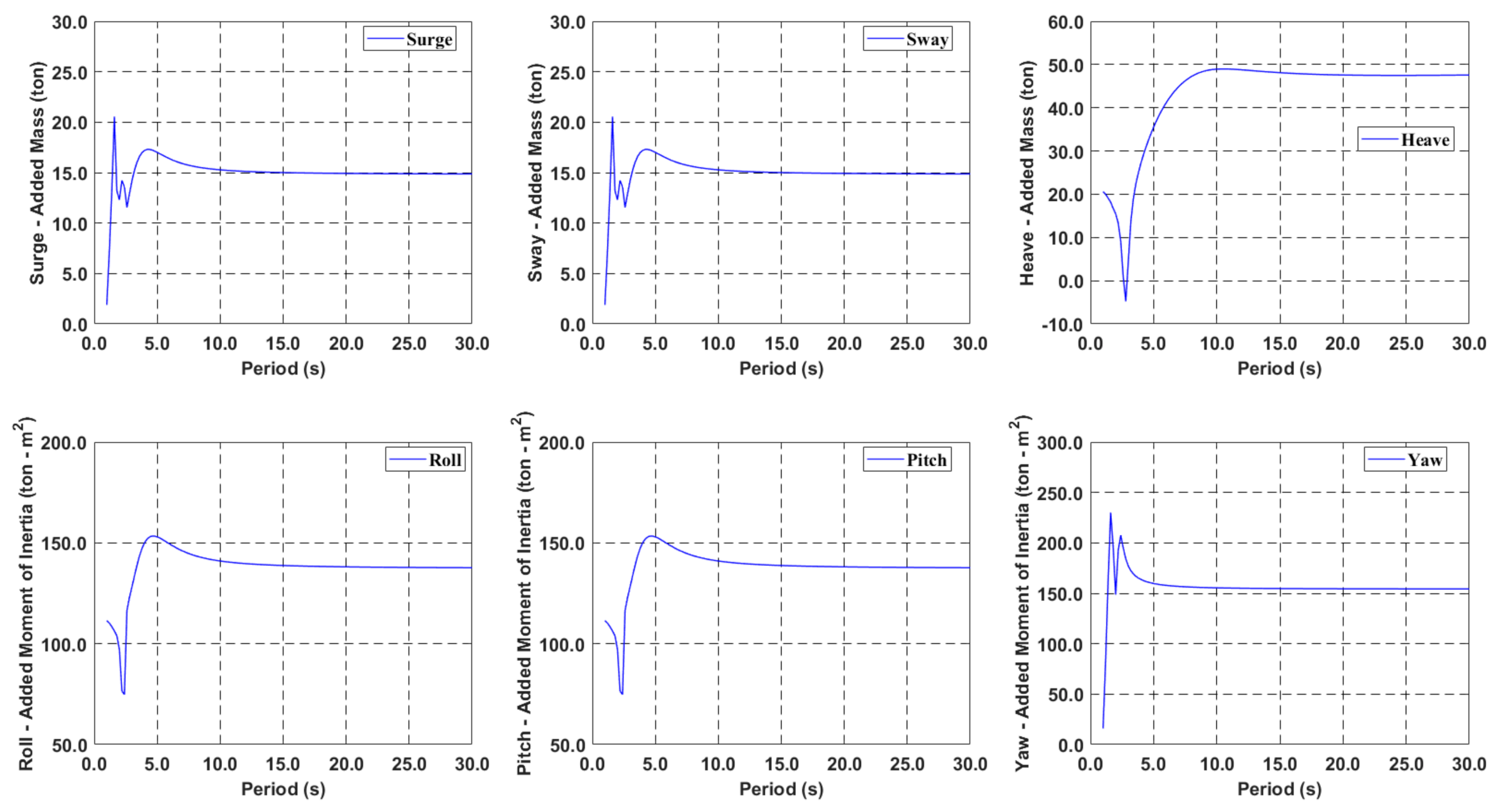
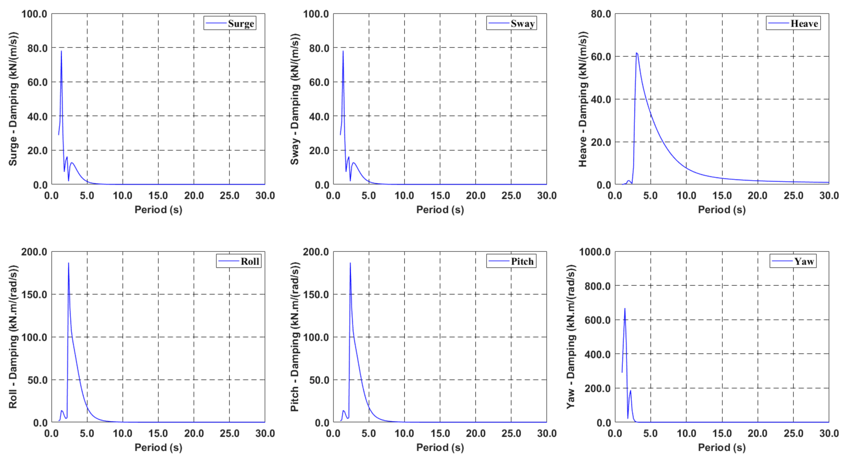
2.1. Hydrodynamic Coefficients (Frequency-Domain Analysis)

For the dynamic analysis of floating structures, the added mass load, due to pressure variations around a body (system of nine cylinders with panels and frames), should be conducted; since a body is oscillating in the water, it causes the surrounding fluid to move. Thereafter, this additional mass (or inertia), due to the fluid moving together, is added to the body, which is an acceleration function of the body.

Furthermore, the hydrodynamic damping load, owing to the dynamic behavior of the floating structure, should be considered. In general, generated waves, owing to the dynamic behaviors of the floating structure, can weaken incident waves; thus, it is known as radiation damping, which is a result of waves generated by body (system of nine cylinders with panels and frames) motions.

The generalized equation for the added mass and radiation damping in OrcaWave with a complex form can be expressed as shown in Equation (1).

$$M_{a,}{}_{ij}-\frac{i}{\omega }{C}_{r,ij}=\rho {{\displaystyle \iint }}_{S_B}{n}_i{\phi }_{j}dS$$

(1)

where $\rho$ is the density of water, $\omega$ is wave frequency, and $n_i, {\phi }_j$ is the normal velocity and radiation potential, respectively. In addition, $M_a$ and $C_r$ are the added mass and radiation damping, respectively. The added mass and radiation damping can be obtained by integrating the pressure induced by the radiation potential on the wetted surface.

A hydrostatic restoring load occurs, owing to buoyancy variations, owing to the motions of the structure. Hydrostatic restoring coefficients are dependent on the hull geometry. For example, when there is heave motion in the dynamic condition, the additional force with the waterplane area (A) occurs, due to the additional buoyancy, which is a function of the heave motion. This force is called the hydrostatic restoring force, and the hydrostatic restoring coefficients ($K_h$) can be calculated by following Equations (2)–(8)

$$K_{h,33}=\rho g{{\displaystyle \iint }}_{S_B}{n}_{z}dS$$

(2)

$$K_{h,34}=\rho g{{\displaystyle \iint }}_{S_B}y{n}_{z}dS$$

(3)

$$K_{h,35}=-\rho g{{\displaystyle \iint }}_{S_B}x{n}_{z}dS$$

(4)

$$K_{h,44}=\rho g{{\displaystyle \iint }}_{S_B}{y}^2{n}_{z}dS+\forall \rho g{z}_b-mg{z}_g$$

(5)

$$K_{h,45}=-\rho g{{\displaystyle \iint }}_{S_B}xy{n}_{z}dS$$

(6)

$$K_{h,55}=\rho g{{\displaystyle \iint }}_{S_B}{x}^2{n}_{z}dS+\forall \rho g{z}_b-mg{z}_g{K}_{h,46}=-\rho g\forall x_b+mg{x}_g$$

(7)

$$K_{h,56}=-\rho g\forall y_b+mg{y}_g$$

(8)

where $K_{h,ij}=K_{h,ji}$ for all i and j in the above, except for $K_{h,46}$ and $K_{h,56}$, and all other values of indices, $K_{h,ij}=0$. Here, i and j are six-element arrays of indices, where i = 1, 2, 3 correspond to the surge, sway, and heave translational modes, while j = 4, 5, 6 to the roll, pitch, and yaw rotational modes, respectively. The symbols $\forall$ and ($x_b,y_b,z_b$) represent the displaced volume and coordinates of the center of buoyancy of the body (system of nine cylinders with panels and frames).

Owing to the complexity of 3D shaped bodies, such as floating solar panel facilities, hydrodynamic coefficients cannot be analytically computed. Thus, a 3D diffraction/radiation program (ex. OrcaWave) should be used to acquire these terms. The added mass and radiation damping are frequency-dependent values.

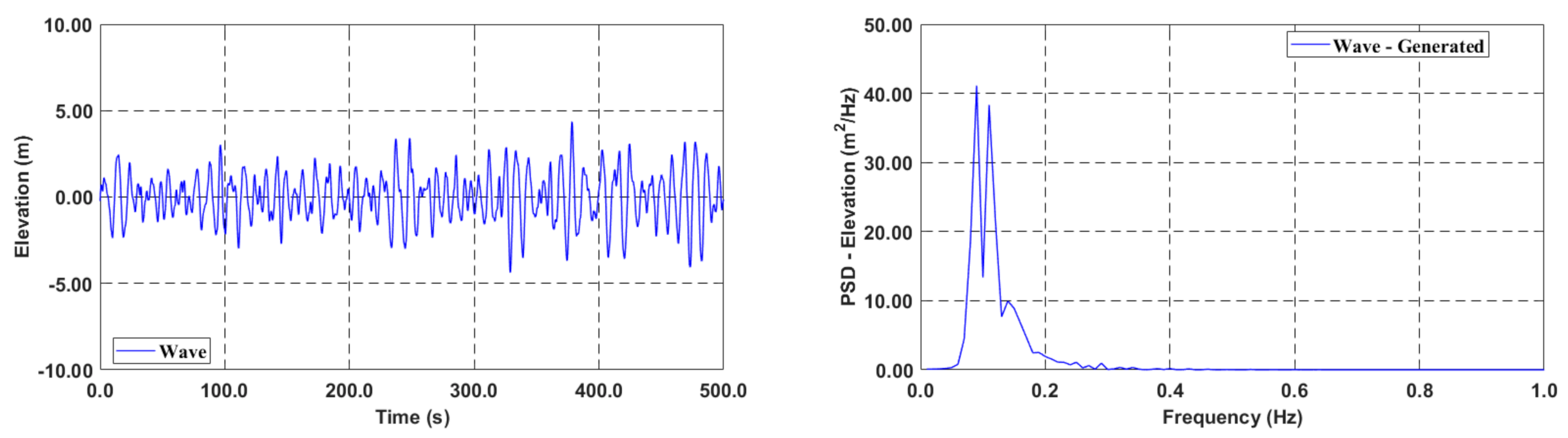
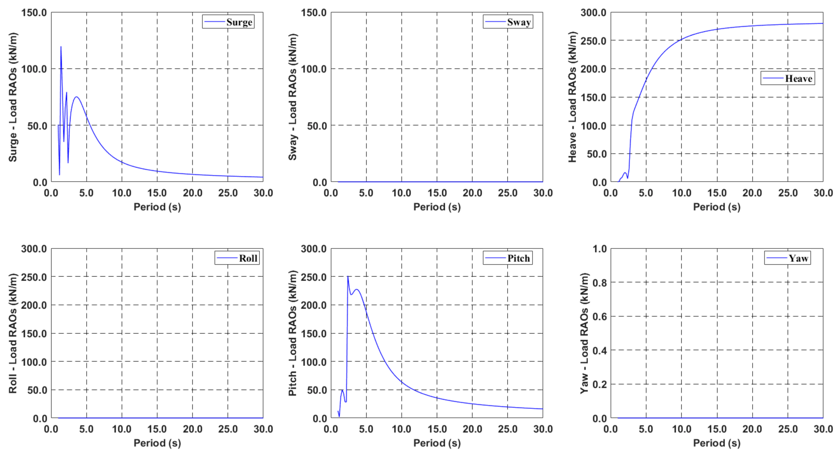
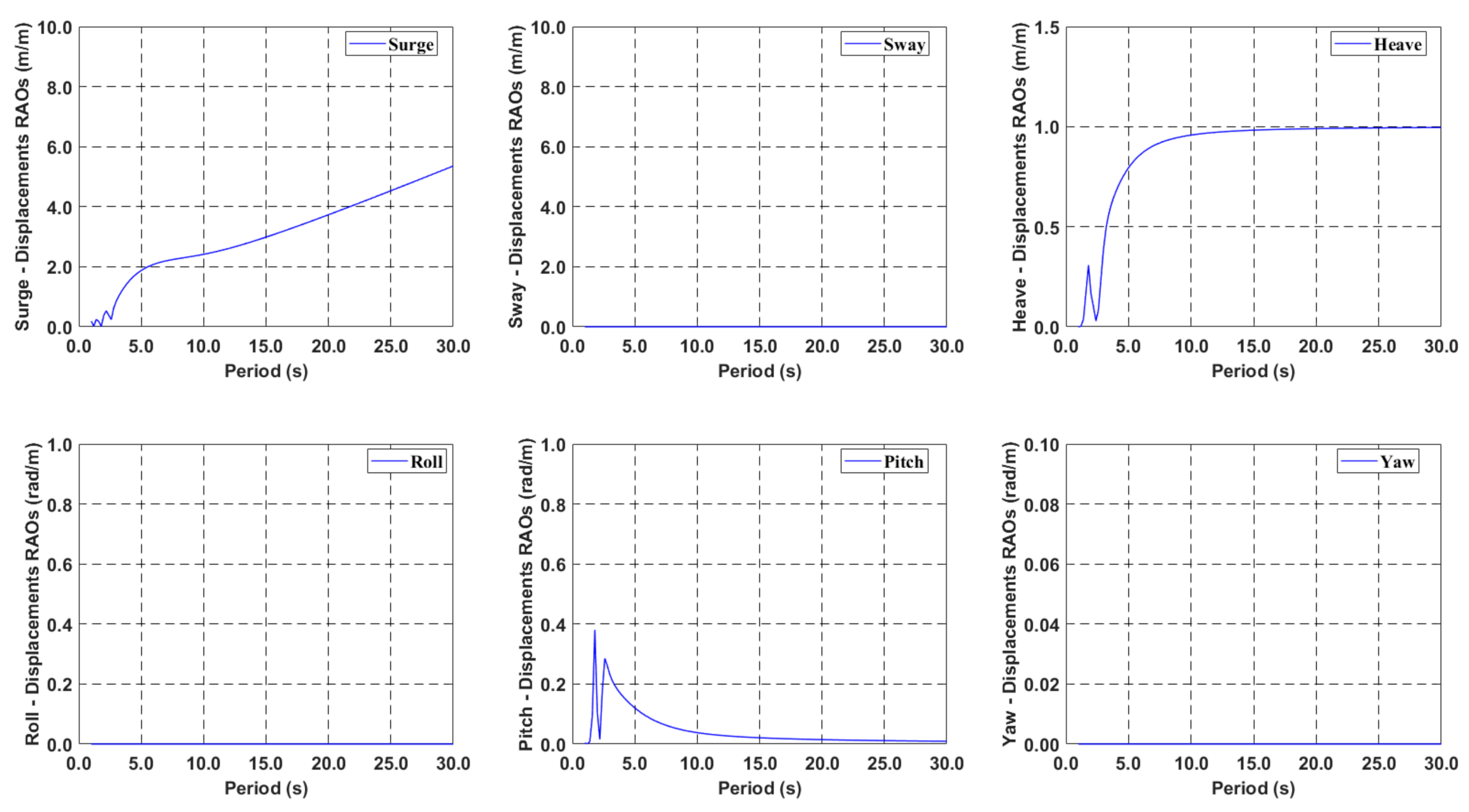
2.2. Wave Excitation Force

Wave excitation force can be divided into two categories: Froude–Kriloff and diffraction wave force. The Froude–Kriloff force term can be defined as the integral pressure on the wetted surface of the structure in the undisturbed wave, as shown in Equation (9).

$$F_{fk}={{\displaystyle \iint }}_{S_B}{p}_{d}nds$$

(9)

In addition, a diffraction occurs around the body (system of nine cylinders with panels and frames) because the wave field near the structure is disturbed. For example, the vertical diffraction force can be estimated by Equation (10), assuming that wavelengths are larger than the characteristic length of the structure:

$$F_{d,3}=M_{a,33}·a_3$$

(10)

where $a_3$ is the vertical wave acceleration.

The 3D diffraction/radiation program should be used to acquire the wave excitation force because the complex geometry of the floating solar panel facility can make it impossible to derive the wave excitation force (no analytical solution). The complex form of the wave excitation force can be expressed as shown in Equation (11):

$$F_w=-i\omega \rho {{\displaystyle \iint }}_{S_B}{n}_i\left({\phi }_0+{\phi }_s\right)dS$$

(11)

where ${\phi }_0$ and ${\phi }_s$ are the incident and scattered wave potentials, which correspond to the Froude–Kriloff and diffraction wave forces, respectively.

2.3. Dynamics of Floating Systems (Time-Domain Analysis)

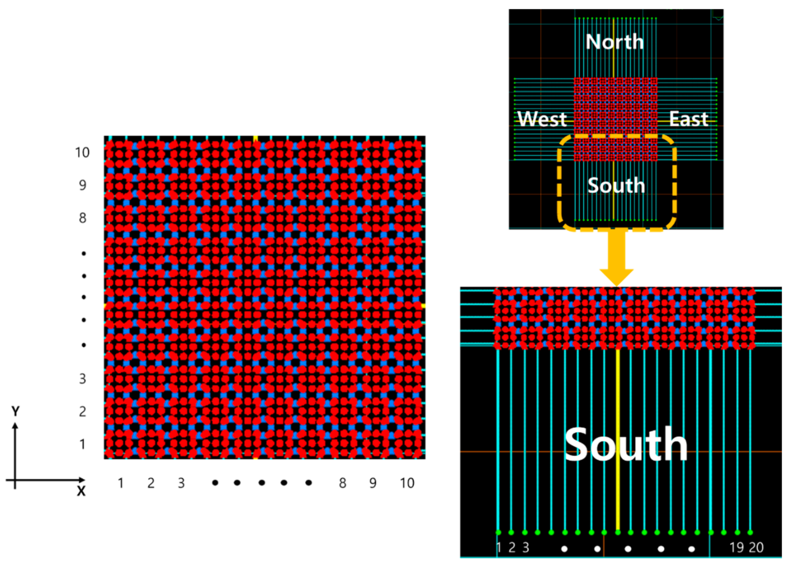
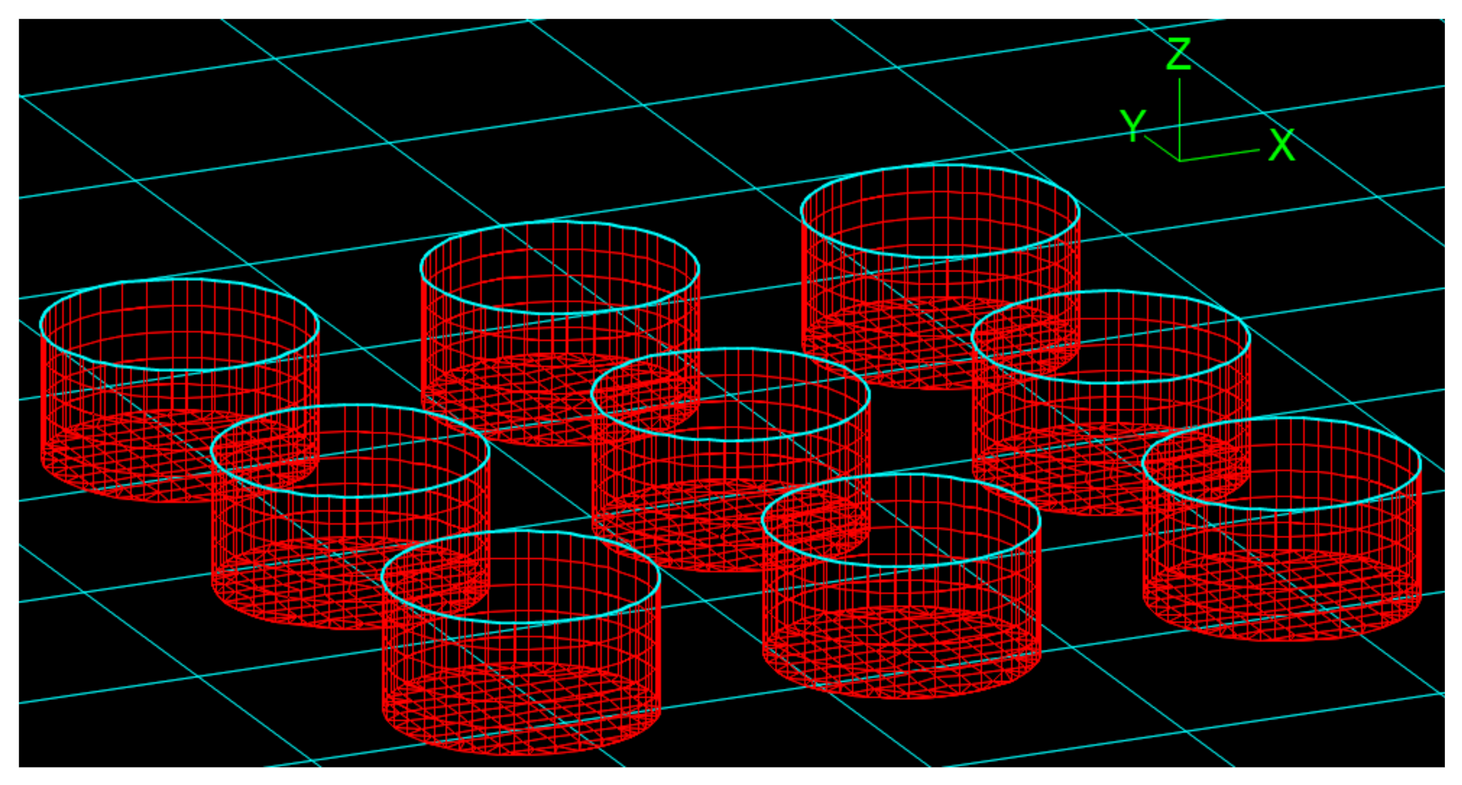
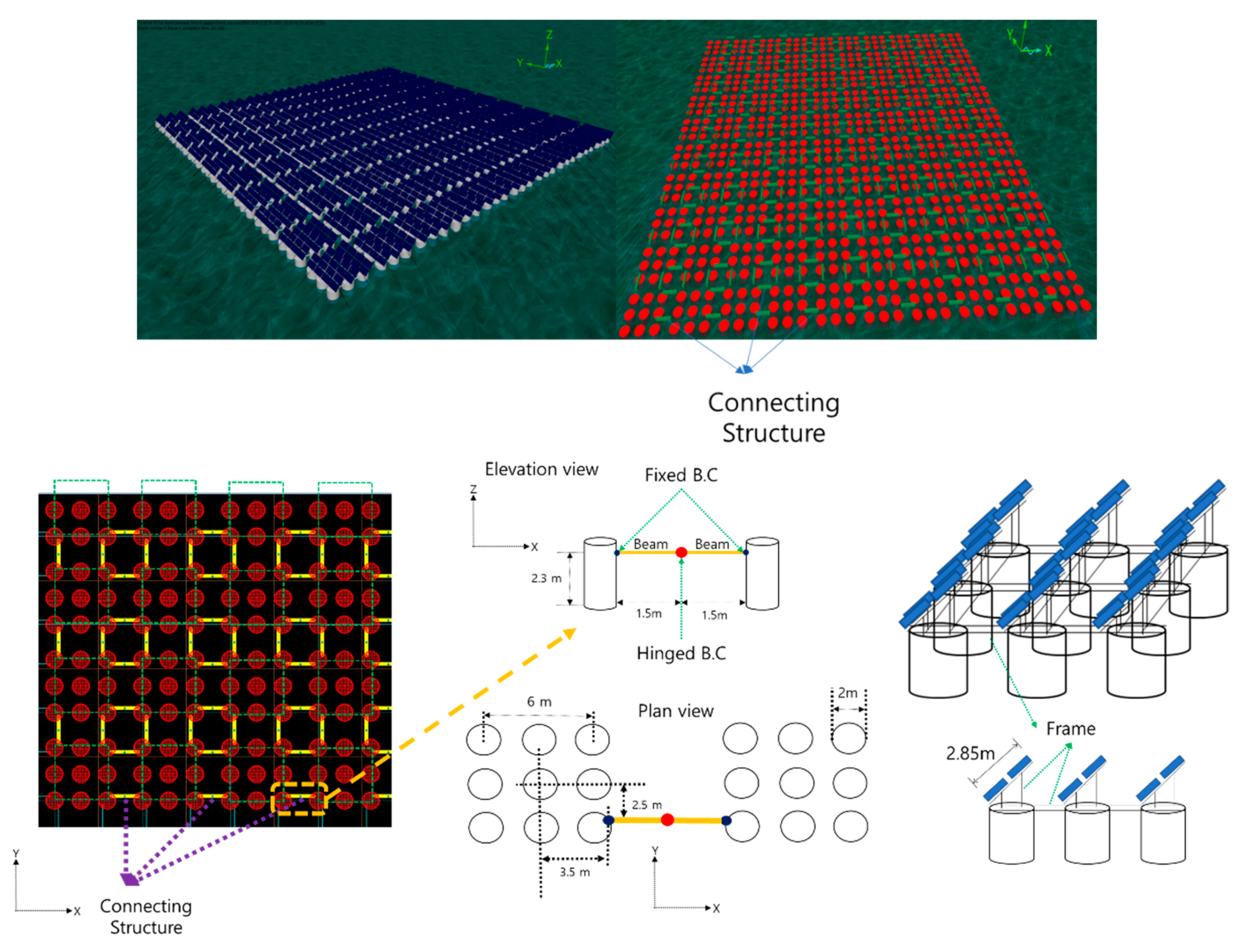
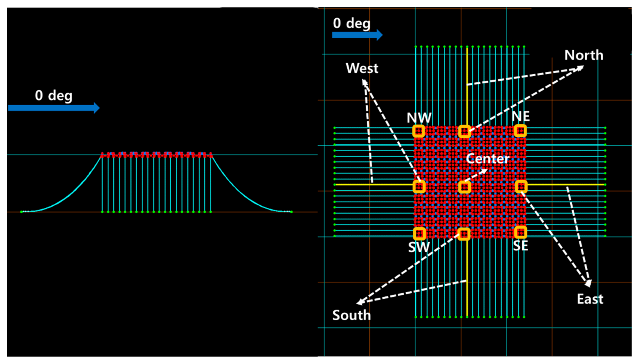
When the nonlinear time-domain approach is used, the equation of motion can be expressed as follows:

$$\left[M+M_a\left(\infty \right)\right]\ddot{\zeta }+{{\displaystyle \int }}_0^{t}R\left(\tau \right)\left(t-\tau \right)d\tau \dot{\zeta }+\left(K_h+K_s\right)\zeta =F_w^{\left(1\right)}$$

(12)

$$M_a\left(\infty \right)=M_a\left(\omega \right)+{{\displaystyle \int }}_0^{\infty }R\left(t\right)\frac{\sin \left(\omega t\right)}{\omega }dt$$

(13)

$$R\left(t\right)=\frac{2}{\pi }{{\displaystyle \int }}_0^{\infty }{C}_r\left(\omega \right)\cos \left(\omega t\right)d\omega$$

(14)

where $M_a$ and $C_r$ are the added mass and radiation damping matrices, respectively; $K_h$ is the hydrostatic restoring stiffness matrix; $\zeta$, $\dot{\zeta }$, and $\ddot{\zeta }$ are displacement (at the center of mass location), velocity, and acceleration, respectively; and $F_w^{\left(1\right)}$ is the first-order wave excitation force. As MLs need to be additionally analyzed with a floating body (system of nine cylinders with panels and frames), additional spring stiffness $K_s$ can be added. In addition, $F_c$ is the radiation damping force, which is obtained by the convolution integral of the retardation function ($R$). The convolution integral accounts for the contribution of frequency-dependent radiation damping.

Continuously, in random waves, the first-order wave load can be expressed using the Volterra series expansion:

$$F_w^{\left(1\right)}=\mathrm{Re}{{\displaystyle \sum }}_{j=1}^N{A}_j{f}_j{e}^{-i{\omega }_{j}t}$$

(15)

where $A$ is the complex wave amplitude, $N$ is the total number of wave components, $f_j$ is the linear force transfer function (LTF), and j is the wave component.

In addition, the connecting structure and MLs can be modeled using line elements. In OrcaFlex, the lumped mass approach was adopted to establish the final equation of motion for the line-based system. The slender line is divided into nodes and segments. Mass, buoyancy, drag, and other properties are lumped at each node, and the nodes are connected by a massless spring that exhibits axial, bending, and torsional properties.

Furthermore, the distributed wave force in a small line element can be estimated using the moving object Morison equation:

$$F_m=C_m\rho \frac{\pi D^2}{4}a-C_a\rho \frac{\pi D^2}{4}{a}_b+\frac{1}{2}\rho C_{d}D\left(v_r\right)\left|v_r\right|$$

(16)

where $C_m$ and $C_a$ are the inertia and added mass coefficients, respectively; $a$, $a_b$, $v_r$ are the acceleration of the fluid, small line element acceleration (relative to global coordinate) and fluid velocity (relative to the small line element), respectively; D is the diameter of small line element, and $C_d$ is the drag coefficient. During the OrcaFlex simulation, an implicit scheme (generalized-α integration scheme), using a constant time step, is selected to solve the equation of motion. A more detailed explanation of the program can be found in the OrcaFlex manual [24].

3. Target Model

As explained previously, hydrodynamic coefficients (added mass/inertia, radiation damping, load response amplitude operator (RAO), and displacement RAO) are required to analyze dynamic responses of the floating system. In this study, a frequency-domain simulation was conducted using OrcaWave. The geometric panel mesh for the floating solar panel system is shown in Figure 1. The floating solar panel system comprises of nine single-unit cylinders, arranged in parallel (horizontally and vertically, 3 m apart from each other). The pontoon (group of nine cylinders) are connected to each other with a frame, so that they can oscillate together. Additionally, in this study, the pontoon (nine cylinders with panels and frames) is considered as rigid. Additionally, as shown in Figure 1, hydrodynamic coefficients are computed based on a set of nine cylinders with 6DOF (degrees of freedom). The specifications of the floating solar panel system are listed in

Table 1. Specification of the base model of the floating solar panel facility with vertical cylinders.

Name		Unit	Value
Mass		ton	3.0578
Center of gravity	X	m	0
	Y	m	0
	Z	m	0.5481
Moment of inertia	Roll	ton-m2	19.068
	Pitch	ton-m2	19.068
	Yaw	ton-m2	35.063

. Moreover, 893 meshes were modelled with quarter symmetry under a 1 m unit length. A wave period of 1–30 s was considered during the numerical simulation, and a wave heading of 0° was considered for comparative analysis. Furthermore, the sea water density and depth were 1025 kg/m³ and 50 m, respectively. In addition, hydrostatic restoring coefficients, which were obtained from the frequency-domain analysis, are listed in

Table 2. Hydrostatic restoring coefficients.

Heave	Roll	Pitch
283.1	0	0
0	1610.7	0
0	0	1610.7

. Figure 2, Figure 3, Figure 4 and Figure 5 show the added mass/inertia, radiation damping, load RAOs, and displacement RAOs under 0°, respectively.

Figure 6 shows the configuration of the base model for the floating solar panel system. The entire system consists of a 10 × 10 floating solar panel pontoon (combined with nine parallel-arranged, single-unit vertical cylinders) and mooring systems. As shown in Figure 7, each mooring group consists of 20 MLs and four mooring groups (80 MLs) are installed to enhance the station-keeping capability. Each ML was modelled using a steel wire rope. The length of each line is 90 m. Details of the mooring material properties are listed in

Table 3. Mooring properties.

Steel Wire
Type	[-]	6 × 19 Wire with Fiber Core
Nominal diameter	[m]	0.15
Mass in air	[kg/m]	81.3
Displaced mass	[kg/m]	12.2
Axial stiffness (EA)	[MN]	825.8
Arc length	[m]	90
MBL (minimum breaking load)	[kN]	11,812.5

. Furthermore, each floating solar panel system is connected to a steel pipe-type connecting structure, and a hinged connector is attached at the connecting point of each steel pipe, while it is fixed at each pontoon. The material properties of the connector are listed in

Table 4. Properties of the connecting structure.

Connecting Structure
Type	[-]	Steel Pipe
Outer diameter	[m]	0.6
Wall thickness	[m]	0.2
Mass in air	[kg/m]	1972.9
Axial stiffness (EA)	[MN]	53,281.4
Bending stiffness (EI)	[MN-m2]	1332.0

. The configurations of the environmental heading, floater dynamic response, and mooring tension measuring locations are plotted in Figure 7. Considering heading directions, floater dynamic responses were measured in nine locations: northwest (NW), north (N), northeast (NE), west (W), center, east (E), southwest (SW), south (S), and southeast (SE). For mooring tension, four lines are selected at the north, south, west, and east, and it is measured at fairlead, which connects the floater with the ML. The configuration of the floater and ML numbering is shown in Figure 8. With respect to load cases, two simulation conditions, normal operating and extreme, were selected (

Table 5. Environmental conditions.

	Wave
	Spectrum	Gamma	Significant Wave (Hs)	Spectral Period (Tp)
	(-)	(-)	(m)	(s/Hz)
Normal operating	JONSWAP	2.2	5.5	10.2/0.098
Extreme	JONSWAP	2.2	8.7	17.2/0.058

). In this study, a widely adopted JONSWAP (Joint North Sea Wave Project) spectrum was used for random wave generation, and regular wave components were superimposed for random wave signals. Using the equal energy method (each regular wave component exhibits equal spectral energy), the repetition of the wave signal in the random wave generation process can be avoided. The sharp parameter (gamma) of the wave spectrum is used in Section 2.2. In addition, in this study, the wake effect caused by the parallel layout of the floating solar panel system was not considered. As listed in

Table 6. Natural frequencies.

	1st (Surge, Sway Governed)	2nd (Yaw Governed)
Unit	Hz	Hz
Value	0.04248	0.05306

, based on modal analysis, the natural frequencies of the target system are 0.04248 (1st mode) and 0.05306 Hz (2nd mode). Owing to the geometrical symmetry of the system, the surge and sway direction natural frequencies were identical (Figure 9).

4. Results and Discussion

In this section, numerical simulation results are presented and discussed to verify the dynamic behavior of the multiconnected floating solar panel system. To simulate a floater–connector–mooring fully coupled system, OrcaFlex, a commercial software that is widely adopted in the offshore industry, was used.

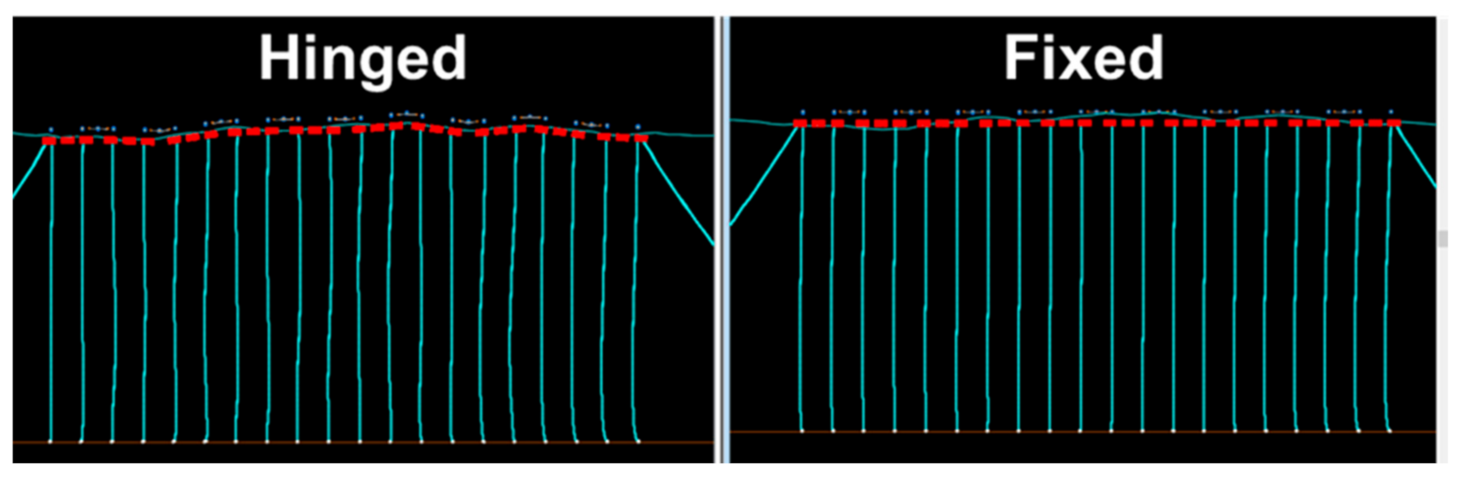
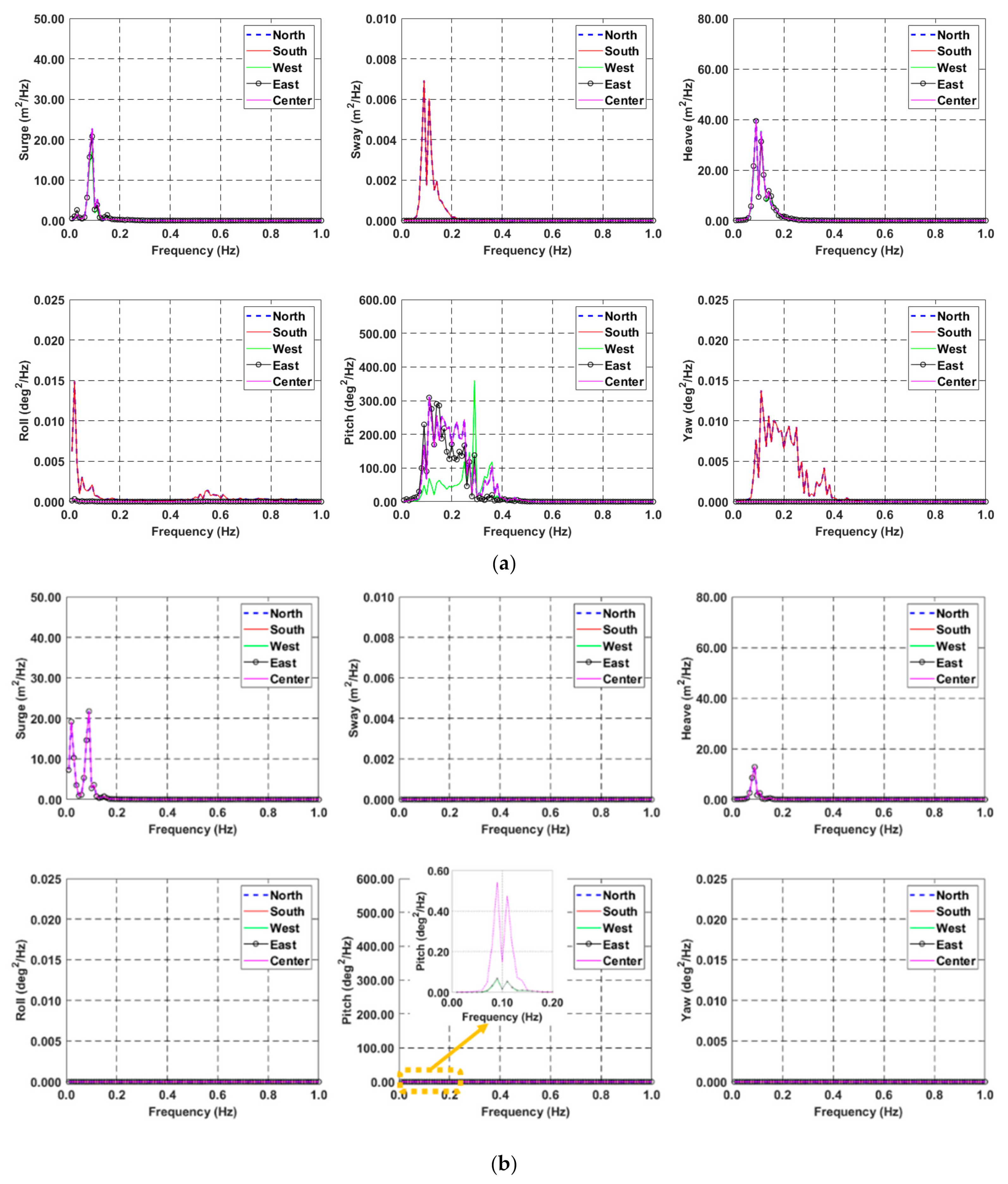
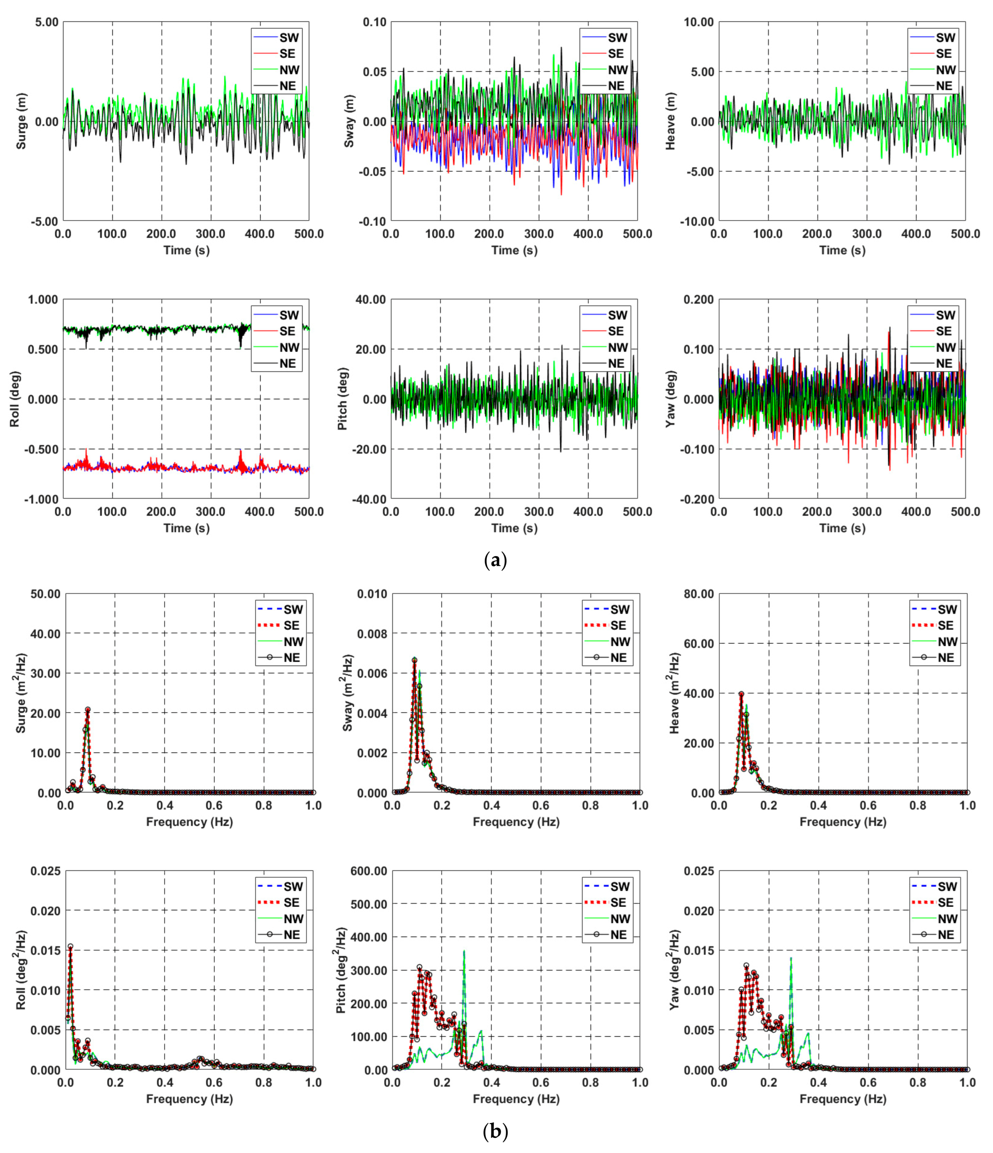
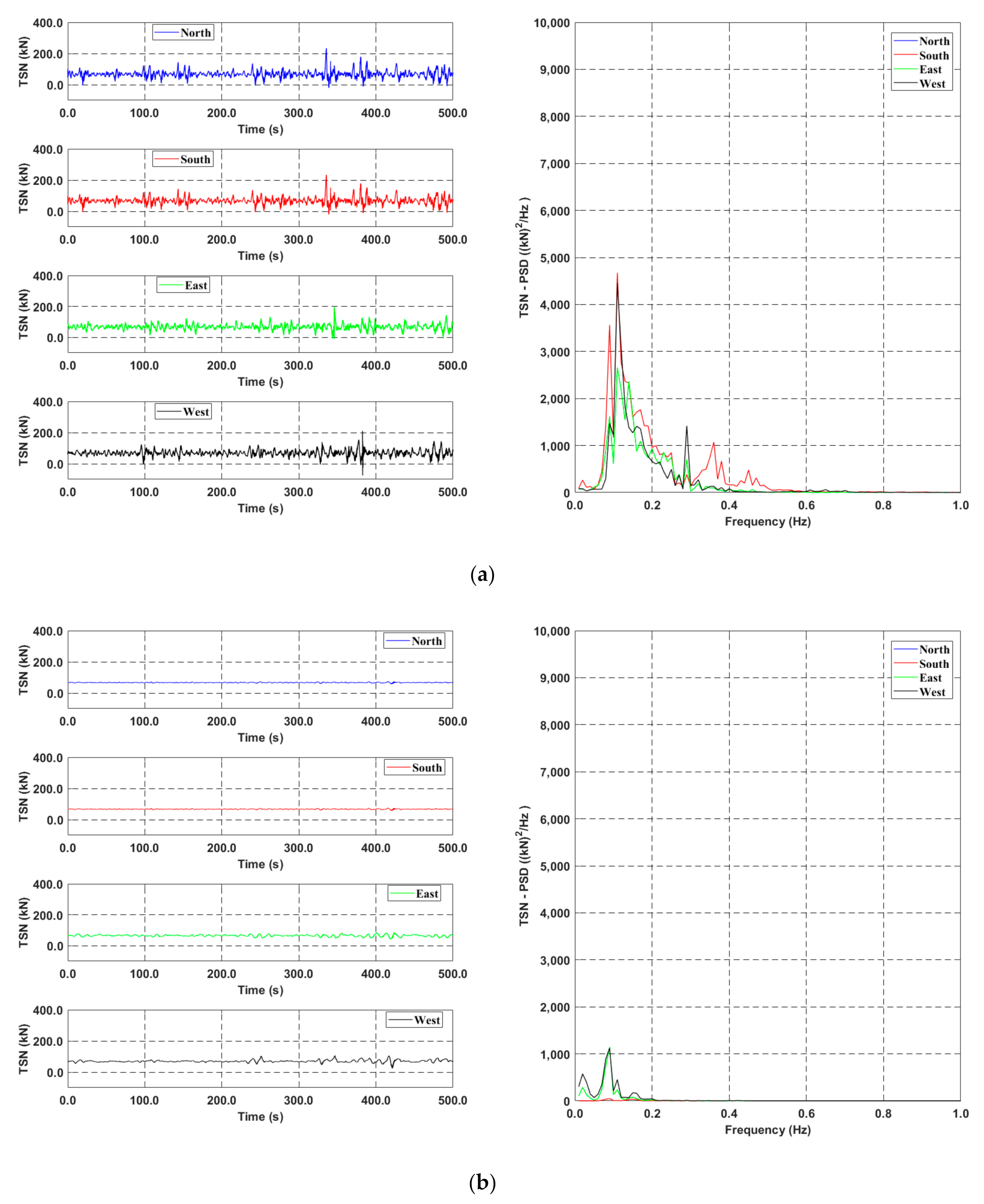
4.1. Connecter Boundary Condition (B.C) Effect (Hinged vs. Fixed)

First, the connector B.C (Boundary Condition) effect is simulated and analyzed. As shown in Figure 10, two connector B.C models were established. In the hinged B.C model, each floating solar panel system moves independently, due to the moment transmission break, whereas the opposite is true with the fixed B.C model. Intuitively, it is expected that this varying moment transmissibility, due to the connector B.C, will cause overall dynamic behavior differences of the multi-connected floating solar panel system.

To check the dynamic response of two different connector B.Cs, both systems are simulated under a normal operating sea state. As shown in Figure 11, the wave elevation time history and corresponding input spectrum under 0° heading are plotted.

The floater motion time history and spectrum comparison results of the north, south, east, west, and center locations are presented in Figure 12 and Figure 13. There were notable dynamic responses along the sway, roll, and yaw directions, while the heading was 0° under the hinged connector B.C, whereas dynamic responses in the same directions could not be observed in the fixed connector B.C case. Furthermore, under fixed B.C, the dynamic responses at all measured locations were almost identical, as evidenced in Figure 12. This is caused by the moment–transmissibility effect. Under the hinged connector B.C case, the additional moment generated by the connector, caused by vertical or rotational movement of the facility, will affect the dynamic behavior of other facilities as another external excitation load. Furthermore, this unexpected dynamic response was observed in the north and south locations. This unexpected dynamic response was caused along the middle direction facility (east-center-west) under 0° heading. Thus, as further evidence, additional results at the corners (NE, NW, SE, and SW) are plotted in Figure 14. Unexpected dynamic responses at the corners (NE, NW, SE, and SW) were caused by the additional moment generated by the connector, due to the vertical or rotational movement of the system.

Figure 15 shows the corresponding mooring tension results of four locations (north, south, east, and west). Due to the dynamic response difference, the mooring tension variation of the hinged connector B.C was greater than that of the fixed connector B.C, even though they have similar initial mean tension values. Corresponding statistical characteristic results for floater motion and mooring tension are tabulated in Appendix A.

Intuitionally, as shown in Figure 16, it can be expected that bending moment (or stress) at the joint of the connectors, under the fixed connector B.C case, is significantly large, due to the sagging and hogging response, while the hinged connector B.C case has zero bending moment (or stress).

Based on the presented results, the connector B.C affects the dynamic behavior of the multiconnected floating solar panel system, with regard to floater motion and mooring tension caused by the additional moment generated by the connector, due to vertical or rotational movement of the system. As the hinged connector B.C model is critical for design purposes, the hinged connector B.C model will be considered in the following sections.

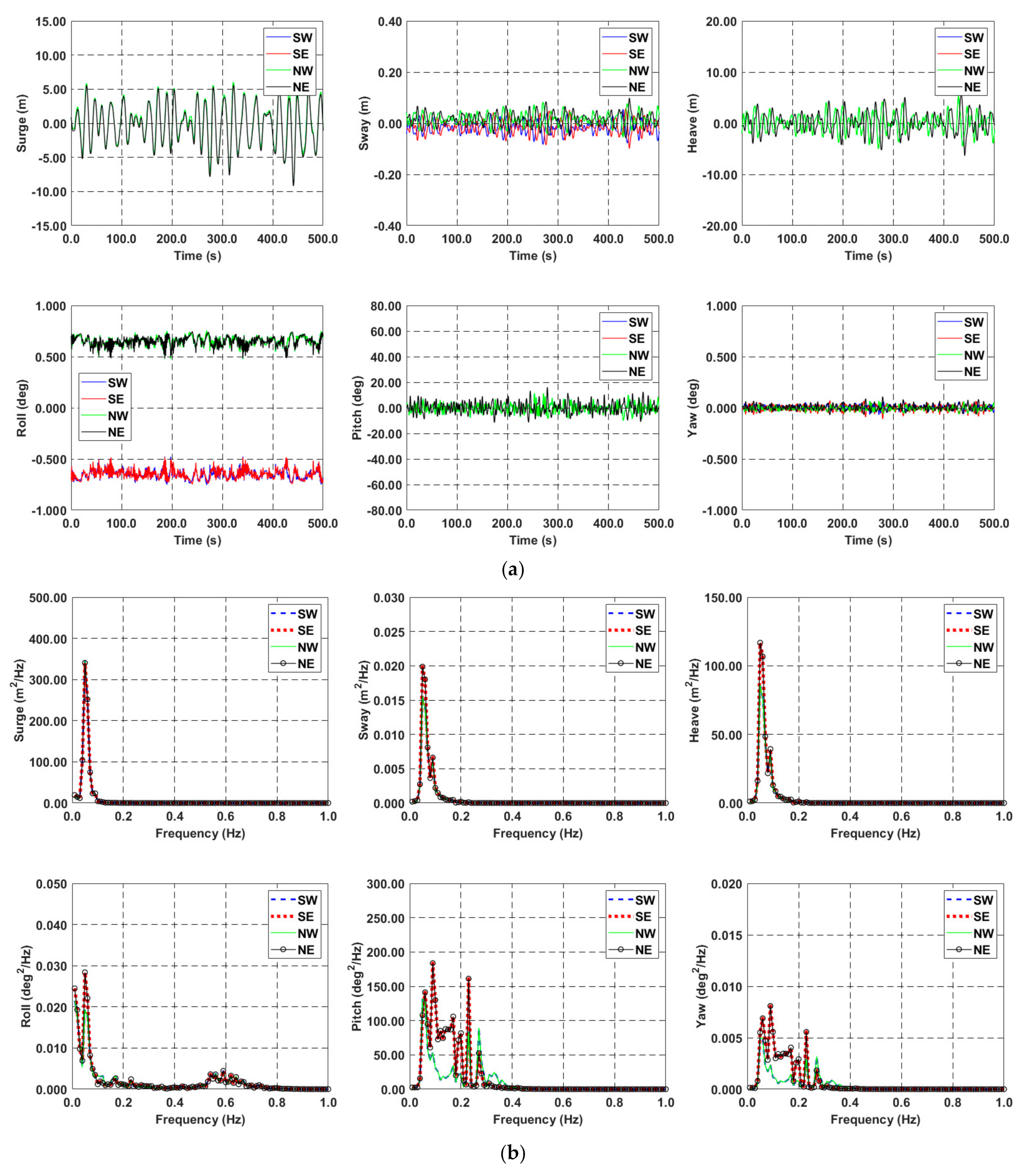
4.2. Extreme Condition

In this section, to confirm the extreme dynamic response of the multiconnected floating solar panel system with vertical cylinders, harsh environmental conditions are considered. Figure 17 shows the extreme wave elevation and its regenerated spectrum under 0° heading.

Floater motions, including each corner, are plotted in Figure 18 and Figure 19. Based on the comparison with normal operating results (Figure 12, Figure 13 and Figure 14), the dynamic response, including the unexpected response along the sway, roll, and yaw directions, is increased, due to the large environmental external loading and resonance effect amplification (due to lower extreme wave peak frequency, compared with the normal operating wave).

Mooring tension results are shown in Figure 20. In addition, the dynamic response of the mooring tension is enhanced, due to the floater motion amplification. Here, the west-ML tension variation significantly increases, compared to other properties. This means that external loading affects mooring dynamics more than the additional moment generated by the connector, caused by the vertical or rotational movement of the system at a certain level of environmental loading, as evidence by the comparison between normal operating and extreme results.

Furthermore, statistical characteristic results are tabulated in Appendix A.

4.3. Multiple Broken MLs

For the floating structure design requirement process, the broken ML case should be tested. Thus, in this section, multiple breaking scenarios of the ML are simulated. As shown in Figure 21, multiple MLs (16 out of 80—4 per group) were intentionally disconnected during the time-domain simulation (at 250 s). The same conditions are considered in Section 4.1 (hinged connector B.C).

Similarly, the floater motion time history and spectrum are plotted in Figure 22 and Figure 23. As expected, the dynamic responses increase, due to the station-keeping load decrement, caused by the ML disconnection. Roll dynamic responses in low- (~0.05 Hz) and high-frequency (~0.55 Hz) regions disappeared after the ML failure (only wave peak frequency was dominant). This is caused by the increase in relative mooring tension at the middle of the north and south locations. Due to its geometry, as tension increases, the floater dynamic response decreases.

The mooting tension comparison results, before and after failure, are presented in Figure 24. The dynamic response and maximum and mean values are significantly amplified after multiple MLs fail.

Similarly, statistical characteristic of ML failure case is summarized in Appendix A.

5. Conclusions

In this study, the dynamic response of a multi-connected floating solar panel system with a vertical cylinder was checked. Based on a single floating solar panel pontoon (combining nine single-unit vertical cylinders, arranged in parallel, horizontally and vertically), the hydrodynamic coefficients were computed. These coefficients were imported into the global performance program. In global performance modeling, multiple floating solar panel pontoon (10 × 10) were connected to each other using a steel pipe connector with a hinged connection in the middle. In this study, the wake effect, due to the parallel arrangement, was not considered. Furthermore, 80 steel wire rope MLs were installed to maintain station-keeping capability. Normal operating and extreme wave conditions were considered environmental loading. For random wave generation, JONSWAP was selected. Based on the present analysis results, the following points were concluded:

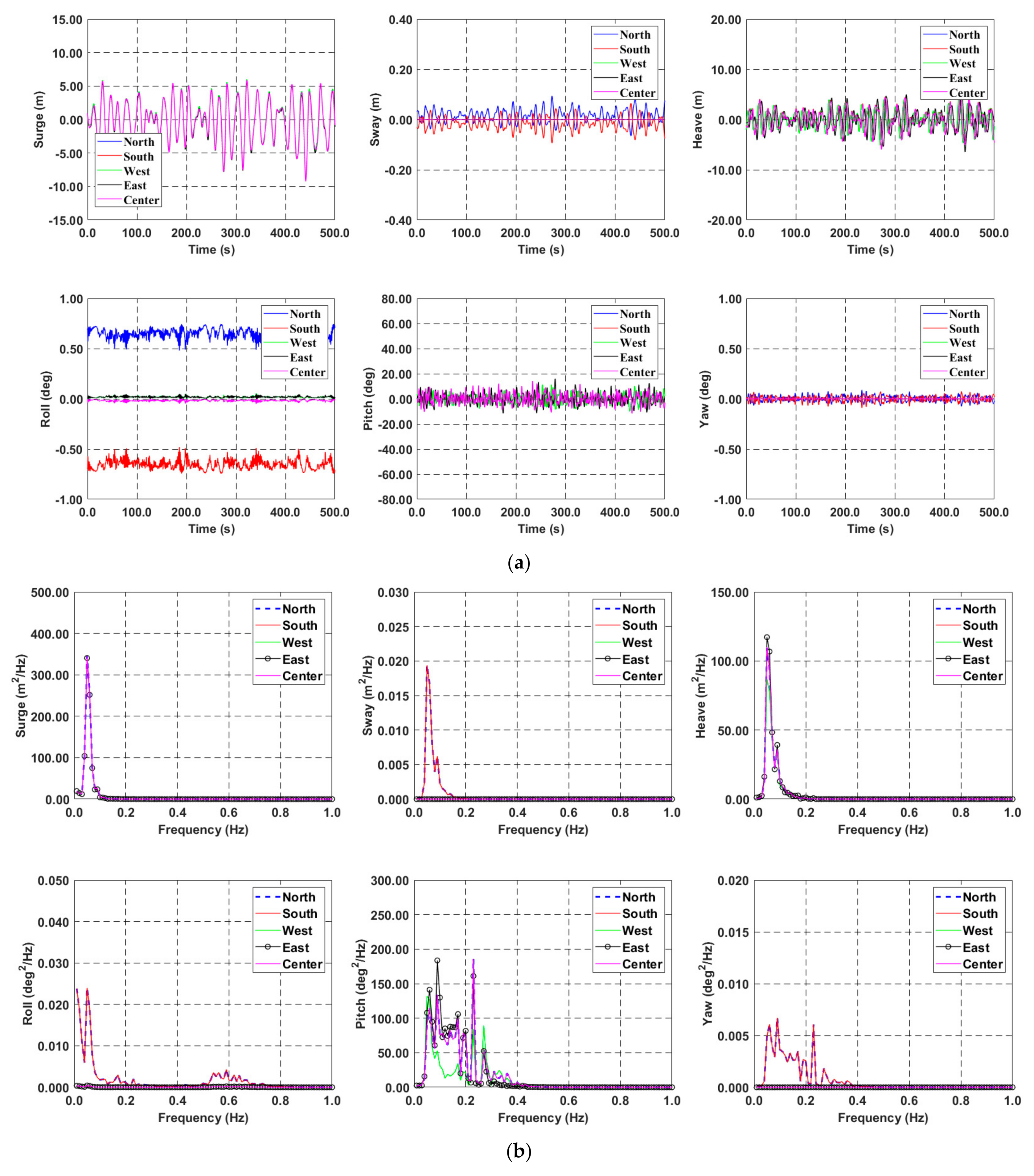
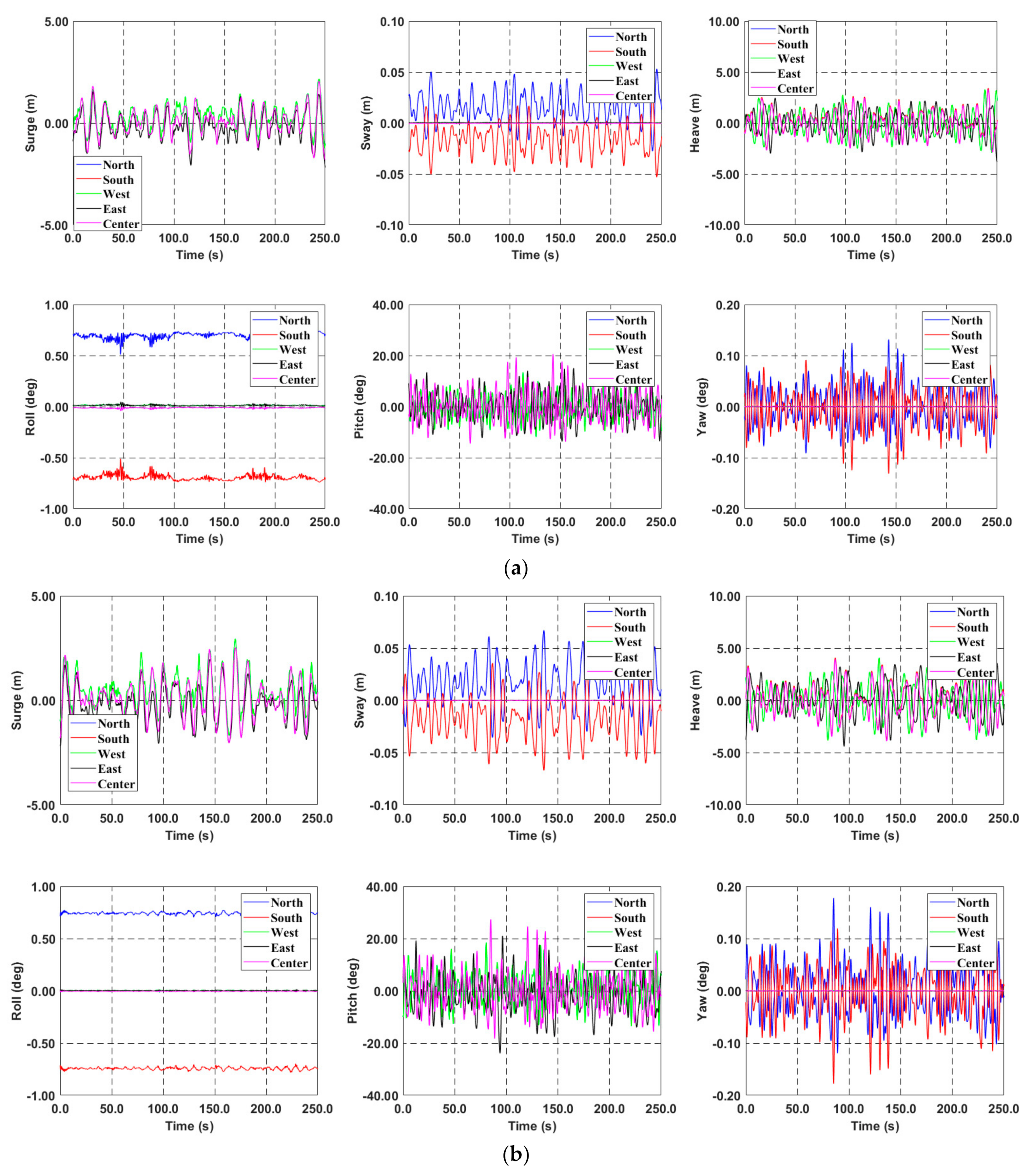
• In normal operation, due to the additional moment generated by the connector, based on the vertical or rotational movement of the system, unexpected dynamic response along the sway, roll, and yaw directions occurred under the hinged connector B.C, whereas it disappeared in the fixed connector B.C case under 0° heading.
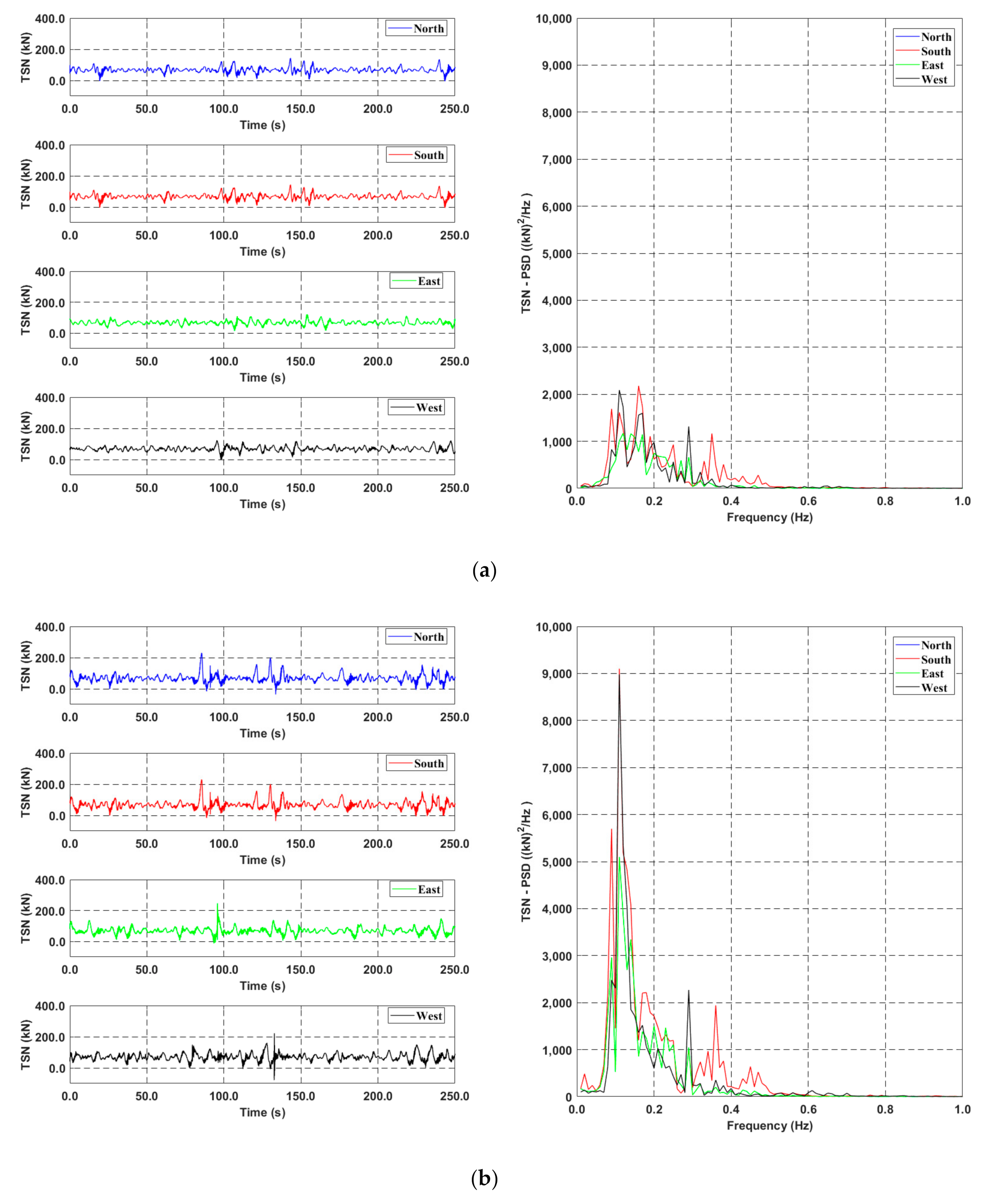
• The mooring dynamics for the hinged connector B.C was greater than that for the fixed connector B.C, and both connectors exhibit similar initial mean values.
• Under extreme wave conditions, the floater dynamic response was amplified, due to the large external loading and resonance effect amplification with a catenary mooring system. In addition, environmental forces (directly affecting the system) significantly influenced the dynamic behavior, rather than the additional moment generated by the connector, based on the vertical or rotational movement of the system at a certain level of external loading.
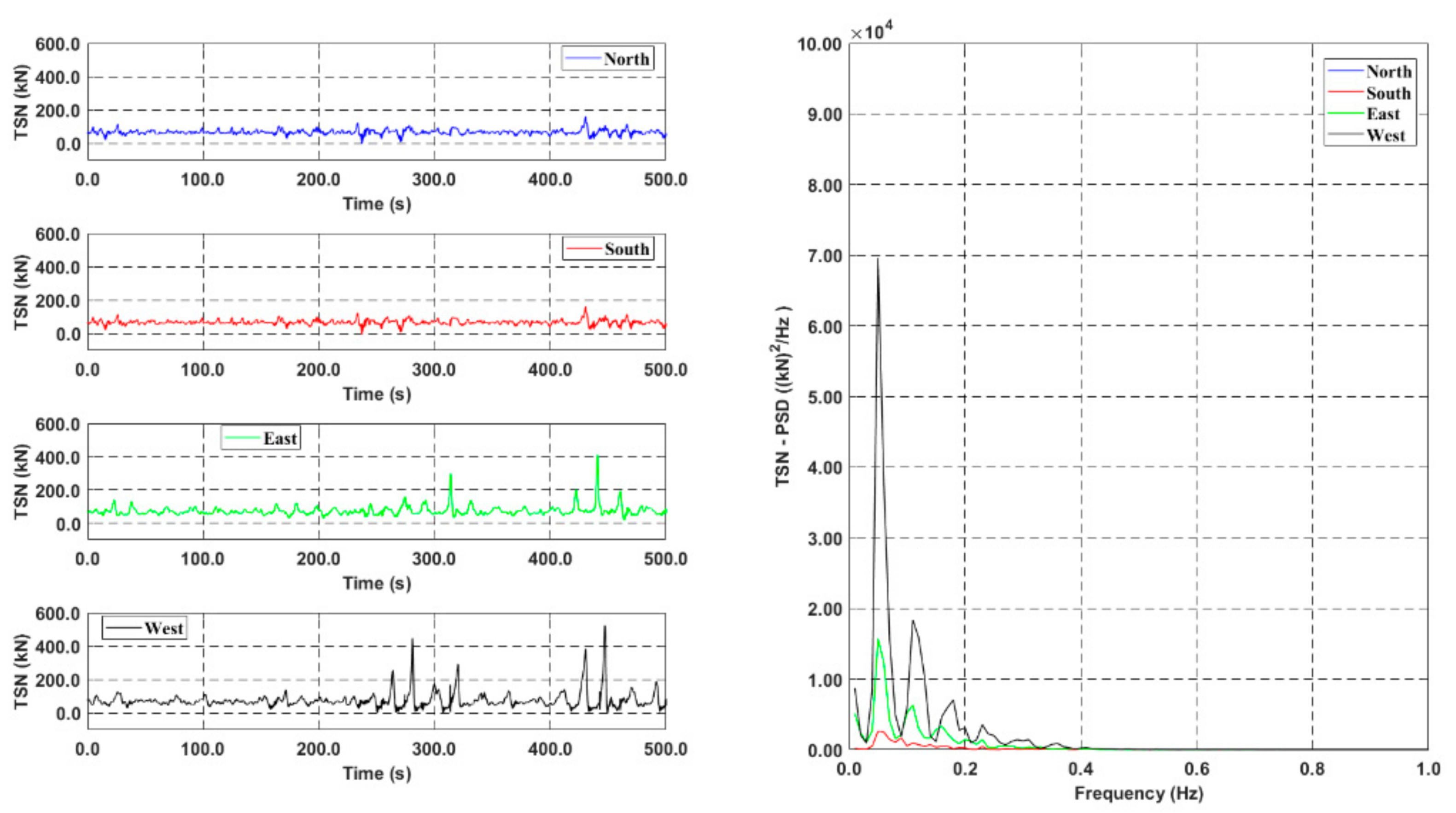
• After multiple failures of the ML, due to the loss of station-keeping load, the dynamic response of the multi-connected floating solar panel system was significantly amplified, and the roll dynamic response decreased, due to an increase in the relative mooring tension at the middle of the location, caused by ML failure.

6. Future Works

In present study, tidal current and wake effects, which might occur potential VIV (vortex-induced vibrations), are not considered. Since those will affect to the dynamic response of the system significantly, those limitations can be considered as a future research topic. Furthermore, design optimization, including mooring systems, will be discussed in the sequel paper.

References

1. Renewables 2020 Global Status Report. (Paris: REN21 Secretariat). 2020. Available online: https://www.globalwomennet.org/renewables-2020-global-status-report/ (accessed on 1 October 2021).
2. Chung, W.C.; Pestana, G.R.; Kim, M. Structural health monitoring for TLP-FOWT (floating offshore wind turbine) tendon using sensors. Appl. Ocean Res. 2021, 113, 102740. [Google Scholar] [CrossRef]
3. Bloomberg New Energy Finance. Global Trends in Renewable Energy Investment 2017. 2017. Available online: https://www.greengrowthknowledge.org/research/global-trends-renewable-energy-investment-2017/ (accessed on 1 October 2021).
4. Sahu, A.; Yadav, N.; Sudhakar, K. Floating photovoltaic power plant: A review. Renew. Sustain. Energy Rev. 2016, 66, 815–824. [Google Scholar] [CrossRef]
5. Oliveira-Pinto, S.; Stokkermans, J. Marine floating solar plants: An overview of potential, challenges and feasibility. Proc. Inst. Civ. Eng. Marit. Eng. 2020, 173, 120–135. [Google Scholar] [CrossRef]
6. Jamalludin, M.A.S.; Muhammad-Sukki, F.; Abu-Bakar, S.H.; Ramlee, F.; Munir, A.B.; Bani, N.A.; Muhtazaruddin, M.N.; Mas’ud, A.A.; Ardila-Rey, J.A.; Ayub, A.S. Potential of floating solar technology in Malaysia. Int. J. Power Electron. Drive Syst. 2019, 10, 1638–1644. [Google Scholar] [CrossRef] [Green Version]
7. Rosa-Clot, M.; Rosa-Clot, P.; Tina, G.; Scandura, P. Submerged photovoltaic solar panel: Sp2. Renew. Energy 2010, 35, 1862–1865. [Google Scholar] [CrossRef]
8. Friel, D.; Karimirad, M.; Whittaker, T.; Doran, W.; Howlin, E. A review of floating photovoltaic design concepts and installed variations. In Proceedings of the 4th International Conference on Renewable Energies Offshore, Lisbon, Portugal, 12–15 October 2020; pp. 1–10. [Google Scholar]
9. Friel, D.; Karimirad, M.; Whittaker, T.; Doran, J. Hydrodynamic investigation of design parameters for a cylindrical type floating solar system. In Proceedings of the 4th International Conference on Renewable Energies Offshore, Lisbon, Portugal, 12–15 October 2020; pp. 763–770. [Google Scholar]
10. Cazzaniga, R.; Cicu, M.; Rosa-Clot, M.; Rosa-Clot, P.; Tina, G.; Ventura, C. Floating photovoltaic plants: Performance analysis and design solutions. Renew. Sustain. Energy Rev. 2018, 81, 1730–1741. [Google Scholar] [CrossRef]
11. Dai, J.; Zhang, C.; Lim, H.V.; Ang, K.K.; Qian, X.; Wong, J.L.H.; Tan, S.T.; Wang, C.L. Design and construction of floating modular photovoltaic system for water reservoirs. Energy 2020, 191, 116549. [Google Scholar] [CrossRef]
12. Clemons, S.K.C.; Salloum, C.R.; Herdegen, K.G.; Kamens, R.M.; Gheewala, S.H. Life cycle assessment of a floating photovoltaic system and feasibility for application in Thailand. Renew. Energy 2021, 168, 448–462. [Google Scholar] [CrossRef]
13. Temiz, M.; Javani, N. Design and analysis of a combined floating photovoltaic system for electricity and hydrogen production. Int. J. Hydrogen Energy 2020, 45, 3457–3469. [Google Scholar] [CrossRef]
14. Al-Yacouby, A.; Halim, E.R.B.A.; Liew, M. Hydrodynamic analysis of floating offshore solar farms subjected to regular waves. In Advances in Manufacturing Engineering; Springer: Berlin, Germany, 2020; pp. 375–390. [Google Scholar]
15. Ravichandran, N.; Ravichandran, N.; Panneerselvam, B. Performance analysis of a floating photovoltaic covering system in an Indian reservoir. Clean Energy 2021, 5, 208–228. [Google Scholar] [CrossRef]
16. Michailides, C.; Loukogeorgaki, E.; Angelides, D.C. Response analysis and optimum configuration of a modular floating structure with flexible connectors. Appl. Ocean Res. 2013, 43, 112–130. [Google Scholar] [CrossRef]
17. Ikhennicheu, M.; Danglade, B.; Pascal, R.; Arramounet, V.; Trébaol, Q.; Gorintin, F. Analytical method for loads determination on floating solar farms in three typical environments. Sol. Energy 2021, 219, 34–41. [Google Scholar] [CrossRef]
18. Kim, S.-H.; Baek, S.-C.; Choi, K.-B.; Park, S.-J. Design and installation of 500-kW floating photovoltaic structures using high-durability steel. Energies 2020, 13, 4996. [Google Scholar] [CrossRef]
19. Kim, S.-H.; Yoon, S.-J.; Choi, W. Design and construction of 1 MW class floating PV generation structural system using FRP members. Energies 2017, 10, 1142. [Google Scholar] [CrossRef] [Green Version]
20. Choi, J.-Y.; Hwang, S.-T.; Kim, S.-H. Evaluation of a 3.5-MW floating photovoltaic power generation system on a thermal power plant ash pond. Sustainability 2020, 12, 2298. [Google Scholar] [CrossRef] [Green Version]
21. Trapani, K.; Millar, D.L. Floating photovoltaic arrays to power the mining industry: A case study for the McFaulds lake (ring of fire). Environ. Prog. Sustain. Energy 2016, 35, 898–905. [Google Scholar] [CrossRef]
22. Choi, Y.-K.; Lee, N.-H.; Lee, A.-K.; Kim, K.-J. A study on major design elements of tracking-type floating photovoltaic systems. Int. J. Smart Grid Clean Energy 2014, 3, 70–74. [Google Scholar] [CrossRef] [Green Version]
23. Orcina. Orcawave User Manual; Orcina: Ulverston, UK, 2021. [Google Scholar]
24. Orcina. Orcaflex User Manual; Orcina: Ulverston, UK, 2006. [Google Scholar]
Figure 1. Panel mesh for the base model of the floating solar panel facility with vertical pontoons.
Jmse 10 00189 g001
Figure 2. Added mass and moment of inertia of the base model.
Jmse 10 00189 g002
Figure 3. Radiation damping of the base model.
Jmse 10 00189 g003
Figure 4. Load RAOs of the base model, 0°.
Jmse 10 00189 g004
Figure 5. Displacement RAOs of the base model, 0°.
Jmse 10 00189 g005
Figure 6. Configurations of the base model and connecting structure.
Jmse 10 00189 g006
Figure 7. Heading and measuring locations.
Jmse 10 00189 g007
Figure 8. Configurations of the floater and mooring line (ML) numbering.
Jmse 10 00189 g008
Figure 9. Natural frequencies and mode shape.
Jmse 10 00189 g009
Figure 10. Configuration of the connecter condition effect (hinged vs. fixed).
Jmse 10 00189 g010
Figure 11. Wave elevation and spectrum, normal operation, 0°.
Jmse 10 00189 g011
Figure 12. Motion, time history, connecter condition effect, hinged (a) vs. fixed (b), normal operation, 0°.
Jmse 10 00189 g012
Figure 13. Motion (power spectral density), connecter condition effect, hinged (a) vs. fixed (b), normal operation, 0°.
Jmse 10 00189 g013
Figure 14. Motion at corner, time history (a) and PSD (b), connecter condition effect, hinged, normal operation, 0°.
Jmse 10 00189 g014
Figure 15. Mooring tension (TSN), connecter condition effect, hinged (a) vs. fixed (b), normal operation, 0°.
Jmse 10 00189 g015
Figure 16. Bending moment at connecter joint (Center), fixed connecter condition, normal operation, 0°.
Jmse 10 00189 g016
Figure 17. Wave elevation and spectrum, extreme, 0°.
Jmse 10 00189 g017
Figure 18. Motion, hinged connector, time history (a) vs. PSD (b), extreme, 0°.
Jmse 10 00189 g018
Figure 19. Motion at corner, hinged connector, time history (a) vs. PSD (b), extreme, 0°.
Jmse 10 00189 g019
Figure 20. TSN, hinged connector, extreme, 0°.
Jmse 10 00189 g020
Figure 21. Configuration of broken MLs.
Jmse 10 00189 g021
Figure 22. Motion, ML broken, time history, hinged connector, before failure (a) vs. after failure (b), normal operating, 0°.
Jmse 10 00189 g022
Figure 23. Motion, ML broken, PSD, hinged connector, before failure (a) vs. after failure (b), normal operation, 0°.
Jmse 10 00189 g023
Figure 24. TSN, ML broken, hinged connector, before failure (a) vs. after failure (b), normal operation, 0°.
Jmse 10 00189 g024