Abstract
The three-dimensional scour beneath a partially-buried pipeline in regular waves was visualized using a miniature camera installed in a transparent pipeline. The scour mechanism was analyzed based on the results. Scour development was observed to start at the upstream edge of the span shoulder when the flow in the span headed downstream. The nearby sediment scoured quickly, and a new scour front formed, which can be attributed to the deflected flow entering the scour hole. The new scour front retreated gradually. The end of the original scour front deformed and moved downstream, probably due to the enhanced seepage flow near the edge of the span shoulder. After that, the new scour front extended to the downstream interface of the sediment and the pipeline, and continued to retreat until the first half of the scour process ended. In the second half of the scour process, the sediment transportation occurred in a similar but mirror-imaged manner. The scour hole propagation rate was also determined based on visualization. The results show that the scour hole propagation rate under a pipeline decreases with an increasing pipeline embedment ratio and rises with the KC (Keulegan–Carpenter) number, which is similar to the result of a previous study.
1. Introduction
Pipelines are vital to the offshore oil industry. Submarine pipelines deployed in offshore regions are faced with hydrodynamic forces including waves, tides, and currents. When waves or currents are sufficiently strong, and the seabed is erodible, local scour can appear underneath the pipeline. This can result in the development of a scour hole along the pipeline, leading to a free span. The development of the free span and the vortex shedding may cause pipeline vibration, which is a major cause of pipeline failure.
Many studies have focused on two-dimensional scour beneath a pipeline, wherein the scour process is assumed to occur in the cross-sectional plane of the pipeline. These two-dimensional studies have focused on the mechanism of the onset of scour [1,2], the equilibrium scour depth [3,4,5], and the time scale of scour hole development [6,7,8]. Extensive studies have focused on numerical simulations of the two-dimensional scour process under a pipeline [9,10,11,12].
Practically, a scour hole develops in both vertical and spanwise directions, so it is three-dimensional. Studies on two-dimensional scour cannot reveal scour development in a spanwise direction. Some research has been conducted on three-dimensional scour under a pipeline. Cheng et al. [13] studied the scour hole extension rate under a pipeline in unidirectional currents with a series of conductivity probes. It was revealed that in some cases, the scour process can be divided into a primary stage and a secondary stage. The difference between the two phases were later associated with the pressure difference on two sides of the pipeline [14]. An empirical formula for scour rate was also proposed based on parametric analysis. Wu and Chiew [15] identified four dimensionless parameters of the scour hole development process. It was found that the scour propagation rate was almost independent of the Shields number, but theoretical analysis indicates that the scour hole propagation rate is affected by the Shields number [13,16]. Wu and Chiew [17] discussed the mechanism of scour hole extension in steady currents by monitoring the flow pattern adjacent to the span shoulder on an immobilized bed. Zhu et al. [18] investigated the parametric effects on the scour propagation rate under a pipeline in steady currents with a mini camera sealed in a transparent pipeline. The critical velocity for scour hole extension was proposed and analyzed in different cases. To account for waves, Cheng et al. [19] extended the research of Cheng et al. [13] by studying the scour hole extension rate beneath a pipeline in wave-only and combined wave-and-current conditions. The effects of the wave incidence angle, KC (Keulegan–Carpenter) number, pipeline embedment, and velocity ratio were systemically investigated. Field surveys were also used in studies on three-dimensional bed variation near a submarine pipeline [20,21].
Compared to the achievements regarding two-dimensional scour, investigations on three-dimensional scour under a pipeline are much fewer and less comprehensive. Additional investigations are needed to better understand the mechanism involved with the scour development process [22]. In previous studies on three-dimensional scour, many researchers focused on the scour hole propagation rate under different hydrodynamic conditions [13,14,15,18], but reports on the detailed scour mechanism at the edge of a span shoulder are limited [17,23]. Moreover, the literature on the scour mechanism and scour evolution process under a pipeline in waves is even less.
In flume experiments, bed elevation variations near offshore structures are usually measured with various sensors and probes, such as point gauges [24], laser bed profilers and scanners [25,26], ultrasonic distance sensors [27], and optical probes [28]. These techniques are capable of measuring the scour propagation rate under the pipeline, but the movement of the sediment under the pipeline cannot be revealed. Thus, other techniques are needed to further study the mechanism of scour development under a pipeline.
Direct observation is an ideal visualization approach to study bed profile evolution, including three-dimensional scour development under a pipeline. The behavior of the sand particles in the scour propagation process can be revealed and analyzed more comprehensively, and the scour hole expansion rate can also be measured directly. More details in the mechanism of scour hole propagation can be discovered, which helps to better understand the variation pattern of the scour hole expansion rate with parameters discussed in previous studies. Present reports on the direct observation of the scour around structures are limited. Sumer et al. [29] investigated the scour process around a circular pile with a mini camera. Similar techniques can also be seen in Zhu et al. [18,30], Raaijmakers and Rudolph [31], and Schendel et al. [32].
In this study, the scour hole expansion process below a pipeline in regular waves was visualized using a miniature camera enclosed in a sealed, transparent model pipeline. The resulting video clips were examined to reveal scour development over a wave period. The objectives of this study are listed as follows.
- Revealing the elementary scour development mechanism by observing sediment movement under the pipeline;
- Measuring the scour propagation rate based on direct observation;
- Analyzing the effects of the pipeline embedment ratio and the KC number on the scour propagation rate.
The results of this study can contribute to further investigations on the detailed mechanism of scour hole propagation under a pipeline, which can help to better predict the scour propagation rate under a pipeline in various conditions.
2. Experimental Setup
2.1. Experimental Apparatus
The experiments were conducted in a wave and current flume at the Laboratory of Hydraulic and Harbor Engineering, Tongji University. The flume is 50 m long, 0.8 m wide, and 1.2 m deep (Figure 1). The flume is equipped with a multi-functional wave generating system which can produce both regular and irregular waves, with wave periods ranging between 0.5 s and 5.0 s. The waves were generated with a piston-type wave maker installed at the upstream end of the flume. The maximum wave height is about 0.25 m at 0.5 m water depth. In this study, active wave absorption was adopted to mitigate wave reflection. Two independent wave gauges installed inside the wave generation system enable the wave generating system to measure the water surface profile and adjust the movement of the wave maker to minimize the effect of the wave reflection. The side walls of the flume are made of glass and the bottom is made of concrete. A wave-absorbing slope is located at the downstream end of the flume. A sand pit of 2.7 m long and 1.0 m deep is located 20 m downstream of the wave maker. The side walls and the bottom of the sand pit are all constructed of impermeable concrete. The velocity near the bottom of the flume was measured by a Nortek Vectrino high-resolution acoustic velocimeter (ADV) placed 3.0 m upstream of the sand pit. The sampling point of the ADV was located 0.11 m above the bottom of the flume. A wave gauge was set 1.0 m upstream of the ADV. The sand pit was filled with medium sand measuring at d50 = 0.283 mm, with a geometric standard deviation of σg = (d84/d16)1/2 = 1.8. The porosity of the bed sediment is 0.565, and the permeability is 2.8 × 10⁻⁵ m/s.

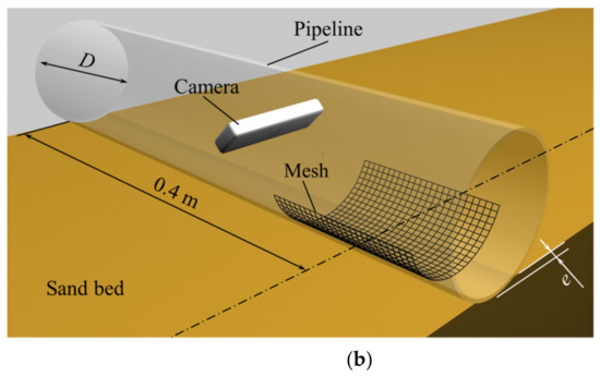
Figure 1.
Schematic plot of experiment setup: (a) experimental flume (side view, not to scale); (b) three-dimensional view of pipeline. Symbols: h0 = water depth; D = pipeline diameter; e = pipeline embedment depth.
The transparent model pipeline is made of Perspex and is 0.11 m in diameter and 0.80 m in length. The pipeline was fixed in the flume with two jack screws at the ends of the pipeline to avoid movement of the pipeline in the tests. A 5-mm mesh was printed on the surface of the pipeline, covering most of the camera’s view [Figure 1b]. A Logitech C920 mini video camera was selected to take videos of the scour development. The resolution of the Full High Definition camera is 1920 × 1080 pixels. The frame rate of the video clips was automatically selected by the camera. In a single video clip, the frame rate was constant. The averaged frame rate of the video clips was 22 fps with a maximum of 30 fps. Two ballast blocks were installed beyond the view of the camera to improve stability. The pipeline was sealed on both ends. The setup of the model pipeline was identical to that used in Zhu et al. [18]. Figure 2 is a typical view of the camera. In Figure 2, Lines AB and CD are the intersections of the initial bed profile and the surface of the pipeline, respectively. The solid line EF is the intersection of the scour hole and the buried part of the pipeline, which is also called the scour front.
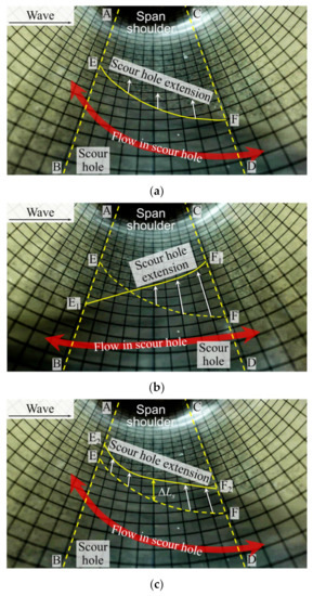
Figure 2.
Typical view of the camera: (a) t = t0; (b) t = t1 (t1 > t0); (c) t = t0 + nT. Symbols: t = time; t0, t1 = two time points in the video clip; T = wave period; n = number of wave periods; ΔLs = distance of the scour hole development at the bottom of the pipeline within n wave periods.
2.2. Dimensional Analysis of Effects on Scour Hole Propagation Rate
Scour under a pipeline in waves is not a steady process. The topography near the scour front is always changing due to the orbital movement of flow near the bed (Figure 2). As a result, a time-averaged scour propagation rate was adopted in this study. The scour propagation rate under a pipeline v0 is defined as:
where ΔLs is the distance of the scour hole development on the bottom of the pipeline within nT and is shown in Figure 2c; n is number of the wave periods, and T is the wave period.
A dimensional analysis was performed to identify the parameters influencing the scour hole propagation rate. The three most important parameters were determined and analyzed based on the results below:
where v* = normalized scour propagation rate, and the normalization method was identical with that used by Cheng et al. [19]; v0 = the scour propagation rate under a pipeline; g = gravitational acceleration (g = 9.8 m/s2); D = pipeline diameter; e = pipeline embedment depth [Figure 1]; KC = Keulegan–Carpenter number; θ = Shields number. The KC number was calculated by:
where Um = maximum value of wave orbital velocity near the bed; T = wave period. The Shields number θ was calculated by the approach used by Cheng et al. [19] derived from Soulsby [33], and:
where τ = shear stress on the bed; ρ = density of the water (ρ = 1.0 × 10³ kg/m3); ρs = density of the sediment particles (ρs = 2.65 × 10³ kg/m3 in this study); d50 = median grain size. The shear stress on the bed induced by waves is calculated by:
where fw = wave friction parameter; ks = Nikuradse equivalent sand grain roughness (ks = 2.5d50).
In this study, the gravity waves over the pipeline were modeled and, thus, Froude’s law was adopted. The scaling ratio was selected as follows. The submarine pipeline deployed in Hangzhou Bay, China was selected as the prototype pipeline, and the diameter of this pipeline is 762 mm. The geometric scale was designed to be model:prototype = 1:6.93, and the corresponding time scale was model:prototype = 1:2.63. Most parameters tested in this study comply with this scaling ratio.
Except for the aforementioned parameters, some other parameters were also found to be important to the variation of the scour propagation rate, including the wave attack angle, relative width of the flume, grain Reynolds number, and geometric standard deviation of the sediment. However, these parameters were either kept constant in all experimental cases or were proved to be less significant, so they were not included in this study.
2.3. Experimental Cases
A total of 12 cases were designed for the visualization analysis on the scour hole development mechanism and scour hole propagation rate in regular waves. The KC number ranged between 2.02 and 5.68 and the pipeline embedment ratio e/D was between 0.045 and 0.182. The Shields number in the tests varied between 0.08 and 0.19. Detailed information for the various experimental cases can be found in Table 1. Case 9 was selected to reveal the scour development process, and Cases 1 to 12 were selected for the analysis on the scour hole propagation rate. The critical Shields number of the sediment is 0.06 and, thus, the cases were all performed in live-bed conditions. The water depth was 0.4 m for all cases. According to the wave parameters in Table 1, the water depth was limited compared with the wave amplitude, but the wave amplitude was far smaller than the wave length. Thus, the waves were slightly non-linear. To simplify the problem, linear wave theory was selected in this study. The parameter values selected for analysis are based on an overall consideration of the experiment’s accuracy, the observation of sediment behavior, the experiment’s setup, and the parameters used in former studies [2,19]. The other parameters were kept constant in different cases.

Table 1.
Test conditions.
Before each test case, the sediment under the pipeline within the coverage of the mesh was removed and replaced gently. Then, the bed was leveled carefully. A similar arrangement was adopted previously by Sumer et al. [2] and Zhu et al. [34]. After that, an initial scour hole was dug beneath the model pipeline at about 15 cm from the edge of the camera view, thus ensuring that scour would begin at this specified point in all cases. When the scour hole extended into the view of the camera, the scour hole propagation rate was steady. If the scour development started at other locations, the test case would be repeated, and the video clip was discarded. The initial scour hole was set in the same way as that in Zhu et al. [18], where more detailed information on the setup of the initial scour hole can be found. Similar techniques can be seen in Cheng et al. [13,19].
In each test case, the data and camera recording started after the water surface was still. The wave generator was started thereafter. The movement of the sediment under the pipeline was observed carefully when the scour front entered the view of the camera. The video recording and the wave generator were not stopped until all the sediment in the camera view was scoured. All the video clips cover at least five complete wave periods. Each test case was repeated at least twice, to minimize random error. After the tests, the frames were extracted from the video clips for further analysis.
3. Scour Hole Extension Process in a Wave Period
In this study, the scour hole extension mechanism was analyzed based on direct observation with a miniature camera installed in a transparent pipeline. Test Case 9 was selected for the mechanism analysis, and the parameters of the regular waves were: wave height H = 0.1 m, wave period T = 2.0 s, and water depth h0 = 0.4 m. The KC number of the waves was 5.68 (Table 1).
Figure 3 shows the variation of the water surface profile and the near-bottom velocity. The theoretical solutions of linear waves are also plotted. The result shows that the variation of the wave profile was slightly non-linear, as is mentioned in Section 2.3. However, the variation of the near-bottom velocity, an important factor of scour under a pipeline, coincides well with the linear theory. This result indicates that it is appropriate to approximate our system using the linear theory in this mechanistic study, and the error due to this simplification is negligible.
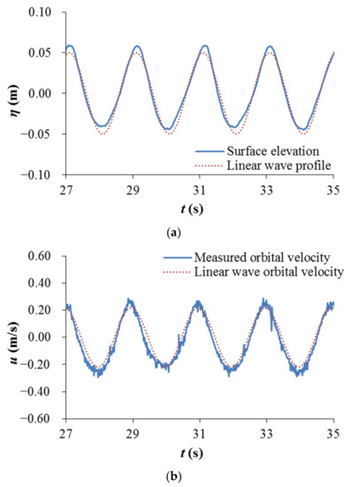
Figure 3.
Measured wave characteristics compared with theoretical linear wave parameters: (a) water surface variation; (b) near-bottom wave orbital velocity.
3.1. Visualization Results
Figure 4 shows a typical scour hole extension process in a wave period (Case 9 in Table 1). The scour front’s curve and the mesh on the pipeline surface were unfolded and included in Figure 4 as a conceptual figure. In Figure 4, the scour process in a wave period was divided into two halves based on the moving direction of the sediment. The sediment moved downstream (from left to right in Figure 4) in the first half of the scour process, and reversed in the second half. The scour process started at t = 63.088 s, when the sand particles in the scour hole were almost still. The phase φ at this point is defined as the initial phase φ0. The scour at the span shoulder started at the upstream end of the scour front [point E in Figure 4b]. The sediment adjacent to point E was pushed into the scour hole and a new scour front E1G1 appeared [Figure 4c]. With the flow velocity increasing, the new scour front continuously retreated. At φ = φ0 + 0.622π, the new scour front retreated to E3G3, covering about half of the buried pipeline, and the end of the original scour front G3F started to deform and gradually moved downstream [point G3 in Figure 4e]. The original scour front G3F deformed and swayed to the downstream side. Some sediment scoured from the curve E3G3 may have been deposited on the extended line of E3G3 [the dotted line in Figure 4e]. After that, the original scour front G3F gradually faded and disappeared. The new scour front E4G4 extended to Line CD, the downstream interface of the sediment and the pipeline, and the sediment movement near point G4 continued [Figure 4f]. The new scour front continued retreating as the scour process continued, but the sediment movement at the downstream end of the scour front gradually slowed down [Figure 4f,g]. During this part of the scour process, the scour front retreated unevenly on the upstream and downstream sides. The movement of point F on the downstream side was faster than that of point E on the upstream. At φ = φ0 + 1.166π, the sediment movement at the span shoulder stopped, and the first half of the scour process in the wave period ended [Figure 4h].
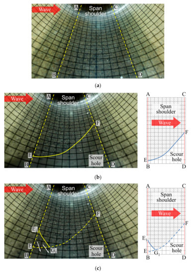
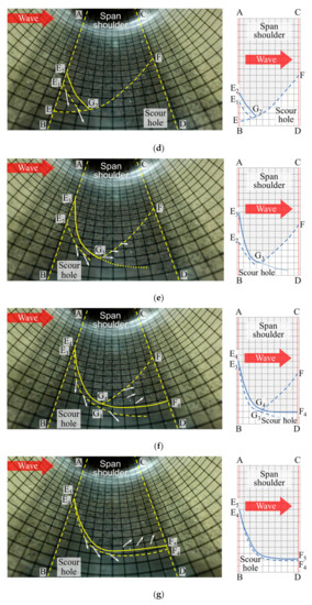
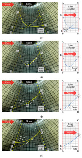
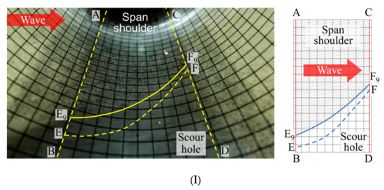
Figure 4.
Typical view of the camera: (a) before the test; (b) φ = φ0 = ω ∙ 63.088 s; (c) φ = φ0 + 0.368π; (d) φ = φ0 + 0.494π; (e) φ = φ0 + 0.622π; (f) φ = φ0 + 0.832π; (g) φ = φ0 + 0.960π; (h) φ = φ0 + 1.166π; (i) φ = φ0 + 1.456π; (j) φ = φ0 + 1.616π; (k) φ = φ0 + 1.744π; (l) φ = φ0 + 2.034π. Symbols: φ = phase; φ0 = initial phase; ω = angular frequency.
After that, the movement of the sand particles reversed and headed to the upstream side, indicating the start of the latter half of the scour process. The movement pattern was similar to the first half of the scour process, but in a mirror-imaged manner. The sediment near point F6 was scoured first. A new scour front formed and retreated to F7G7 [Figure 4i]. Then the deformation and movement of the original scour front started and the new scour front F8G8 extended to the upstream side [Figure 4i,j]. The new scour front retreated as it did in the first half of the scour process. The scour front retreated a little faster on the upstream side [point E in Figure 4j–l]. A similar phenomenon was also observed in the first half of the scour process. The scour process in this wave period ended at φ = φ0 + 2.034 π. The whole scour process took 2.034 s, which is nearly equivalent to the wave period (T = 2.0 s). This process repeated in the next wave period. Similar phenomena were also observable in the video clips of other test cases.
3.2. Discussion on the Scour Hole Evolution Process
The scour mechanism under a pipeline in steady currents has been discussed in previous studies [14,17,23,35]. The main attribution to scour development under a pipeline is the excessive capacity of sediment transportation at the span shoulder due to the local accelerated flow entering the scour hole [17]. At the edge of the scour hole, the local flow accelerates due to the topography of the pipeline and the scoured bed, and the bed shear stress and the sediment transportation capacity rise dramatically [35]. Besides a local increase in the shear stress, the scour process is also associated with some other attributions such as the variation of sediment parameters and seepage in local sediment [14]. The dominant cause of scour development under a pipeline in waves is similar. However, the scour hole development in waves is a far more complex process than that in steady currents. When the pipeline is subject to regular waves, the flow in the span is approximately an oscillating flow. The frequent change in the flow direction significantly affects the sediment transportation at the end of the span shoulder and, thus, the scour development. In this section, the aforementioned scour process in a wave period is discussed and analyzed.
At the beginning of the scour process, the sediment around point E [Figure 4b] was scoured and a new scour front formed. The scour that initiated at point E can be expounded by the diversion of the accelerating near-bottom flow on the upstream side of the span shoulder. On the upstream side of the pipeline, the near-bottom flow near the scour front was deflected towards the scour hole due to the pipeline and local topography while accelerating [17]. Thus, the sediment at point E was scoured first, and the scour front E1G1 was approximately parallel with the deflected near-bottom flow. Similarly, the scour started at point F6 when the sediment movement reversed [Figure 4i].
The original scour front G3F moved and deformed gradually with the retreat of the new scour front E3G3 [Figure 4e], which can be attributed to the excessive seepage flow near point G. A bed pressure difference forms on two sides of the pipeline when near-bottom flow passes over the pipeline [1]. After the sediment under the pipeline is scoured, the pressure difference does not simply disappear. Instead, the pressure difference decreases slightly when the scour front is approaching this cross section, and the drop rate increases when the scour front arrives at the cross section. After that, the pressure difference drops steadily [14]. Thus, when the new scour front retreated gradually from E1G1 to E3G3 [Figure 4e], the pressure difference across the pipeline at point G still existed, although it was smaller than that before the scour front approached. Meanwhile, the length of the seepage path near point G decreased significantly due to the scour. As the length of seepage path decreased and the pressure difference was still remarkable, the seepage hydraulic gradient and the seepage force in the sediment near point G could rise remarkably, pushing the sediment downstream.
In Figure 4g, the scour front was witnessed to retreat unevenly. This may be attributed to the relatively low density of the sediment on the downstream side. When the scour front E4F4 extended to the downstream interface of the sediment and the pipeline CD [Figure 4f], the sediment in the area FF4G4 was not as compact as the undisturbed sediment, sometimes even containing hollow sections. This phenomenon is more remarkable when the pipeline embedment is larger or the KC number is smaller, and the hollow sections in the area FF4G4 can be clearly observed. The sediment in this area was scoured during the previous wave period. The movement and deformation of the original scour front G3F pushed some sand into the scoured part but was unable to refill it before the sediment stopped moving. The sediment compactness was lower than that of the undisturbed soil, and the sediment was more vulnerable to scour. Thus, the scour front near F4G4 moved faster. The uneven movement of the scour front in the second half of the scour process [Figure 4k,l] can be similarly explained. As the regular waves in this study were slightly non-linear, the near-bottom flow velocity in the second half of the scour process was lower, and the phenomenon was more remarkable. The rapid scour development near point E [Figure 4b] and point F6 [Figure 4h] can also be partially attributed to this phenomenon.
The development of a scour front pattern is affected by hydrodynamic parameters, including the KC number. Xie et al. [23] proposed that the pattern of the scour front inclines more steeply towards the scour hole when the blockage of the pipeline is more significant. A similar phenomenon was also observed in this study. The qualitative observation of the video clips showed that the curve of scour front EG inclined more sharply to the scour hole in cases with larger KC numbers, with other variables fixed. When the KC number is larger, the maximum velocity of the near-bottom flow is higher, and the near-bottom flow lasts for a longer time before reversing. The blockage is, thus, intensified, and the transverse diversion of the approaching flow is more remarkable. Consequently, the scour front can incline more steeply towards the scour hole.
It should be noted that the movement of sand particles cannot represent the movement of water, as the density of sediment particles is much larger than that of water. A phase difference may exist between the orbital movement of the wave and the sediment. When the sediment particles at the span shoulder were still and about to move in the reverse direction, the flow nearby may have reversed and was accelerating in the reverse direction.
4. Parametric Effects on Scour Propagation Rate
4.1. Effect of Pipeline Embedment
Figure 5 shows the variation of the normalized scour propagation rate v* with the pipeline embedment ratio e/D. The pipeline embedment e/D varied between 0.045 and 0.182. The results by Cheng et al. [19] in similar conditions are also plotted. Figure 5 depicts that the scour propagation rate generally decreases with the increase in the pipeline embedment ratio. The results in the present study share a similar trend with Cheng et al. [19], in that the decrease in the scour propagation rate is almost linear when e/D ≥ 0.1 for different KC numbers. The scour rate is more sensitive to the variation of the pipeline embedment when e/D < 0.1, which coincides with previous reports on steady currents [15]. The drop rate of the scour rate gradually slows down as the embedment increases when e/D < 0.1. With the increase in the pipeline embedment, the scour rate is less dependent on the KC number, as the data points with the same e/D but different KC get closer for larger e/D values.
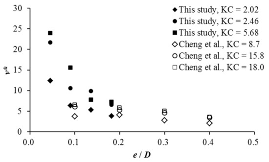
Figure 5.
Variation of normalized scour propagation rate with pipeline embedment.
The variation pattern of the scour propagation rate with the pipeline embedment depth can be attributed to two factors:
On one hand, with the increase in the pipeline embedment, the pipeline blockage effect is less remarkable [1], and the near-bottom flow entering the scour hole decreases. Thus, the capability of sediment transportation of the local flow at the scour front reduces [19].
On the other hand, with the increase in the pipeline embedment depth, a larger part of the pipeline is buried in the sediment. The length of the seepage path climbs accordingly. It is mentioned in Section 3 that the decrease in the length of the seepage path partially contributes the scour process, so the increase in the length of the seepage path can cause a lower scour hole development rate for a larger pipeline embedment.
4.2. Effects of KC Number and Shields Number
Figure 6 depicts the variation of the normalized scour propagation rate with the KC number. The KC number ranges between 2.02 and 5.68. In general, the scour rate under the pipeline increases with the KC number. The scour rate is more sensitive to the KC number for 2 < KC < 3. When the KC number is larger, the scour rate becomes less sensitive.
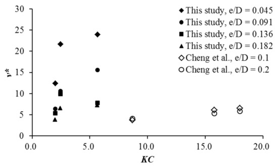
Figure 6.
Variation of normalized scour propagation rate with KC number.
Figure 7 depicts the varying trend of the scour rate with the Shields number. The scour rate increases with the rise of the Shields number, which coincides with the conclusion of Cheng et al. [19]. The rise of the scour rate with the KC number and the Shields number can be explained as follows. The increase in the KC number implies an increase in the maximum near-bottom orbital velocity or a longer time for the near-bottom flow’s effects, or both. With these two factors, the capacity of sediment transportation rises, and the scour rate increases. When the Shields number rises, the capacity of sediment transportation climbs accordingly and, thus, the scour rate ascends.
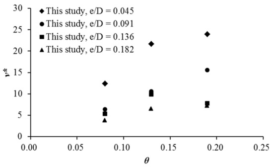
Figure 7.
Variation of normalized scour propagation rate with Shields number.
Figure 6 also includes the results by Cheng et al. [19] in similar conditions. The results in the present study and in Cheng et al. [19] share a similar trend for both parameters. Considering that the pipeline diameter of the present study is much larger than that in Cheng et al. [19], the much smaller data points of Cheng et al. [19] may be attributed to the overestimation of the pipeline diameter effect in the normalization equation (Equation (2)). The difference may also be brought by the difference of other test parameters of the two studies, including the sediment particle size and the geometric standard deviation of the sediment.
Cheng et al. [19] attributed the increase in the scour rate with the KC number to the vortex shedding near the pipeline when KC > 6. In the present study, the KC number is less than 6 for all cases, but the rise of scour rate with the KC number is still remarkable. This phenomenon indicates that some other factors can also affect the variation of scour rate with KC. A possible factor may be the calculation of the KC number. As far as the KC number is concerned, KC is affected by the pipeline diameter, the wave period, and the orbital velocity near the bed (Equation (3)). When the pipeline diameter is held constant, the increase in KC indicates the rise of the wave period or the maximum orbital velocity. The rise of the wave period may trigger the increase in the bed load transportation during each period, thus increasing the scour rate. The climb in the orbital velocity near the bed may enhance the interaction between the sediment and the bottom flow. Thus, the scour rate may also increase.
5. Conclusions
The three-dimensional scour process beneath a pipeline in regular waves was investigated with visualization tests in the present study. The scour development was observed with a miniature camera sealed in a transparent pipeline. The scour process in a wave period was observed and analyzed under regular wave conditions.
At the beginning of the scour process, the scour started at the upstream edge of the span shoulder with the flow in the span heading downstream, which can be attributed to the deflected flow entering the scour hole. The sediment nearby was soon scoured, and a new scour front appeared. After that, the original scour front began to deform and gradually moved downstream, with the new scour front retreating continuously. The scour front extended to the downstream interface of the sediment and the pipeline, which may be associated with enhanced seepage flow near the edge of the span shoulder. Then, the scour front continued retreating gradually until the first half of the scour process ended. In the second half of the scour process, the sediment transportation process reversed, and a similar process occurred but in a mirror-imaged manner.
Parametric analysis showed that the scour propagation rate under a pipeline in waves decreases almost linearly as the pipeline embedment increases, when e/D ≥ 0.1. The scour rate climbs with the KC number at a decreasing rate of increasing, which is consistent with previous research works. The scour rate also increases with the rising Shields number.
Author Contributions
Conceptualization, Y.Z., L.X. and T.-C.S.; methodology, Y.Z., L.X. and T.-C.S.; investigation, Y.Z., L.X., T.W. and T.-C.S.; resources, Y.Z. and L.X.; writing—original draft preparation, Y.Z.; writing—review and editing, Y.Z., L.X. and T.-C.S.; visualization, Y.Z., L.X. and T.W.; supervision, L.X.; funding acquisition, Y.Z. and L.X. All authors have read and agreed to the published version of the manuscript.
Funding
This research was funded by the National Natural Science Foundation of China, grant numbers 11172213 and 51479137, and the China Scholarship Council, grant number 201806260166.
Institutional Review Board Statement
Not applicable.
Informed Consent Statement
Not applicable.
Data Availability Statement
Data from the present experiment appear in the submitted manuscript.
Conflicts of Interest
The authors declare no conflict of interest.
References
- Chiew, Y.M. Mechanics of local scour around submarine pipelines. J. Hydraul. Eng. 1990, 116, 515–529. [Google Scholar] [CrossRef]
- Sumer, B.M.; Truelsen, C.; Sichmann, T.; Fredsøe, J. Onset of scour below pipelines and self-burial. Coast. Eng. 2001, 42, 313–335. [Google Scholar] [CrossRef]
- Chiew, Y.M. Prediction of maximum scour depth at submarine pipelines. J. Hydraul. Eng. 1991, 117, 452–466. [Google Scholar] [CrossRef]
- Dogan, M.; Aksoy, A.O.; Arisoy, Y.; Guney, M.S.; Abdi, V. Experimental investigation of the equilibrium scour depth below submerged pipes both in live-bed and clear-water regimes under the wave effect. Appl. Ocean Res. 2018, 80, 49–56. [Google Scholar] [CrossRef]
- Zhang, Z.; Guo, Y.; Yang, Y.; Shi, B.; Wu, X. Scale model experiment on local scour around submarine pipelines under bidirectional tidal currents. J. Mar. Sci. Eng. 2021, 9, 1421. [Google Scholar] [CrossRef]
- Zhang, Q.; Draper, S.; Cheng, L. Scour below a subsea pipeline in time varying flow conditions. Appl. Ocean Res. 2016, 55, 151–162. [Google Scholar] [CrossRef] [Green Version]
- Zang, Z.; Tang, G.; Cheng, L. Time scale of scour below submarine pipeline under combined waves and currents with oblique incident angle. In ASME 2017, Proceedings of the 36th International Conference on Ocean, Offshore and Arctic Engineering, Trondheim, Norway, 25–30 June 2017; ASME: New York, NY, USA, 2017; p. V009T10A019. [Google Scholar]
- Myrhaug, D.; Ong, M.C. Time scale for scour beneath pipelines due to long-crested and short-crested nonlinear random waves plus current. J. Mar. Sci. Eng. 2021, 9, 114. [Google Scholar] [CrossRef]
- Liang, D.; Cheng, L.; Li, F. Numerical modeling of flow and scour below a pipeline in currents: Part II. Scour simulation. Coast. Eng. 2005, 52, 43–62. [Google Scholar] [CrossRef]
- Zang, Z.; Cheng, L.; Zhao, M.; Liang, D.; Teng, B. A numerical model for onset of scour below offshore pipelines. Coast. Eng. 2009, 56, 458–466. [Google Scholar] [CrossRef]
- Huang, P.; Meng, X.; Dong, H.; Chong, L. Numerical modeling of submarine pipeline scouring under tropical storms. Water 2021, 13, 1425. [Google Scholar] [CrossRef]
- Huang, J.; Yin, G.; Ong, M.C.; Myrhaug, D.; Jia, X. Numerical investigation of scour beneath pipelines subjected to an oscillatory flow condition. J. Mar. Sci. Eng. 2021, 9, 1102. [Google Scholar] [CrossRef]
- Cheng, L.; Yeow, K.; Zhang, Z.; Teng, B. Three-dimensional scour below offshore pipelines in steady currents. Coast. Eng. 2009, 56, 577–590. [Google Scholar] [CrossRef]
- Wu, Y.; Chiew, Y.M. Mechanics of pipeline scour propagation in the spanwise direction. J. Waterw. Port Coast. Ocean Eng. 2014, 141, 04014045. [Google Scholar] [CrossRef]
- Wu, Y.; Chiew, Y.M. Three-dimensional scour at submarine pipelines. J. Hydraul. Eng. 2012, 138, 788–795. [Google Scholar] [CrossRef]
- Draper, S.; Yao, W.; Cheng, L.; Tom, J.; An, H. Estimating the rate of scour propagation along a submarine pipeline in time-varying currents and in fine grained sediment. In ASME 2018, Proceedings of the 37th International Conference on Ocean, Offshore and Arctic Engineering, Madrid, Spain, 17–22 June 2018; ASME: New York, NY, USA, 2018; p. V005T04A019. [Google Scholar]
- Wu, Y.; Chiew, Y.M. Mechanics of three-dimensional pipeline scour in unidirectional steady current. J. Pipeline Syst. Eng. Pract. 2013, 4, 3–10. [Google Scholar] [CrossRef]
- Zhu, Y.; Xie, L.; Su, T.C. Visualization tests on scour rates below pipelines in steady currents. J. Hydraul. Eng. 2019, 145, 04019005. [Google Scholar] [CrossRef]
- Cheng, L.; Yeow, K.; Zang, Z.; Li, F. 3D scour below pipelines under waves and combined waves and currents. Coast. Eng. 2014, 83, 137–149. [Google Scholar] [CrossRef] [Green Version]
- Leckie, S.H.; Draper, S.; White, D.J.; Cheng, L.; Fogliani, A. Lifelong embedment and spanning of a pipeline on a mobile seabed. Coast. Eng. 2015, 95, 130–146. [Google Scholar] [CrossRef]
- Leckie, S.H.; Mohr, H.; Draper, S.; McLean, D.L.; White, D.J.; Cheng, L. Sedimentation-induced burial of subsea pipelines: Observations from field data and laboratory experiments. Coast. Eng. 2016, 114, 137–158. [Google Scholar] [CrossRef]
- Fredsøe, J. Pipeline-seabed interaction. J. Waterw. Port Coast. Ocean Eng. 2016, 142, 03116002. [Google Scholar] [CrossRef] [Green Version]
- Xie, L.; Zhu, Y.; Su, T.C. Visualization tests on variation of scour front under a pipeline in steady currents. J. Mar. Sci. Eng. 2019, 7, 345. [Google Scholar] [CrossRef] [Green Version]
- Saha, R.; Lee, S.O.; Hong, S.H. A Comprehensive Method of Calculating Maximum Bridge Scour Depth. Water 2018, 10, 1572. [Google Scholar] [CrossRef] [Green Version]
- Cui, Y.; Lam, W.H.; Zhang, T.; Sun, C.; Robinson, D.; Hamill, G. Temporal model for ship twin-propeller jet induced sandbed scour. J. Mar. Sci. Eng. 2019, 7, 339. [Google Scholar] [CrossRef] [Green Version]
- Arboleda Chavez, C.E.; Stratigaki, V.; Wu, M.; Troch, P.; Schendel, A.; Welzel, M.; Villanueva, R.; Schlurmann, T.; De Vos, L.; Kisacik, D.; et al. Large-scale experiments to improve monopile scour protection design adapted to climate change—the PROTEUS Project. Energies 2019, 12, 1709. [Google Scholar] [CrossRef] [Green Version]
- Qi, W.; Gao, F. Equilibrium scour depth at offshore monopile foundation in combined waves and current. Sci. China Tech. Sci. 2014, 57, 1030–1039. [Google Scholar] [CrossRef] [Green Version]
- An, H.; Cheng, L.; Zhao, M.; Tang, G.; Draper, S. Detecting scour and liquefaction using OBS sensors. In Scour and Erosion, Proceedings of the 8th International Conference on Scour and Erosion, Oxford, UK, 12–15 September 2016; Harris, J., Whitehouse, R., Moxon, S., Eds.; CRC Press: Boca Raton, FL, USA, 2016; pp. 535–542. [Google Scholar]
- Sumer, B.M.; Hatipoglu, F.; Fredsøe, J. Wave scour around a pile in sand, medium dense, and dense silt. J. Waterw. Port Coast. Ocean Eng. 2007, 133, 14–27. [Google Scholar] [CrossRef]
- Zhu, Y.; Xie, L.; Liang, X. Scour patterns below pipelines and scour hole expansion rate. In Scour and Erosion, Proceedings of the 8th International Conference on Scour and Erosion, Oxford, UK, 12–15 September 2016; Harris, J., Whitehouse, R., Moxon, S., Eds.; CRC Press: Boca Raton, FL, USA, 2016; pp. 387–394. [Google Scholar]
- Raaijmakers, Q.; Rudolph, D. Time-dependent scour development under combined current and waves conditions—Laboratory experiments with only monitoring technique. In Proceedings of the 4th International Conference on Scour and Erosion, Tokyo, Japan, 5–7 November 2008. [Google Scholar]
- Schendel, A.; Welzel, M.; Schlurmann, T.; Hsu, T.W. Scour around a monopile induced by directionally spread irregular waves in combination with oblique currents. Coast. Eng. 2020, 161, 103751. [Google Scholar] [CrossRef]
- Soulsby, R. Dynamics of Marine Sands: A Manual for Practical Applications; Thomas Telford: London, UK, 1997. [Google Scholar]
- Zhu, Y.; Xie, L.; Wong, T.-M.; Su, T.-C. Visualization of the onset of scour under a pipeline in waves. Appl. Sci. 2020, 10, 2994. [Google Scholar] [CrossRef]
- Shen, W.; Griffiths, T.; Zan, Z.; Leggoe, J. Shear stress amplification around subsea pipelines: Part 3, 3D study of spanning pipelines. In Scour and Erosion: Proceedings of the 7th International Conference on Scour and Erosion, Perth, Australia, 2–4 December 2014; Cheng, L., Draper, S., An, H., Eds.; CRC Press: Boca Raton, FL, USA, 2014; pp. 325–335. [Google Scholar]
Publisher’s Note: MDPI stays neutral with regard to jurisdictional claims in published maps and institutional affiliations. |
© 2022 by the authors. Licensee MDPI, Basel, Switzerland. This article is an open access article distributed under the terms and conditions of the Creative Commons Attribution (CC BY) license (https://creativecommons.org/licenses/by/4.0/).