Short-Term Trajectory Prediction of Maritime Vessel Using k-Nearest Neighbor Points

Abstract

The prediction of ship location has become an increasingly popular research hotspot in the field of maritime transportation engineering, which benefits maritime safety supervision and security. Existing methods of ship location prediction based on motion characteristics have a large uncertainty and cannot guarantee trajectory prediction accuracy of the target ship. An improved method of location prediction using k-nearest neighbor (KNN) is proposed in this paper. An expanded circle area of the latest point of the target ship is first generated to find the reference points with similar movement characteristics in the constraints of distance and time intervals. Then, the top k-nearest neighbors are determined based on the degree of similarity. Relationships between the reference point of each neighbor and the latest points of the target ship are calculated. The predicted location of the target ship can then be determined by a weighted calculation of the locations of all neighbors at the predicted time and their relationships with the target ship. Experiments of ship location prediction in 10 min, 20 min, and 30 min were conducted. The correlation coefficient of the location prediction error for the three experiments was 0.992, 0.99, and 0.9875, respectively. The results show that ship location prediction with reference to multiple nearest neighbors with similar movements can provide better accuracy.

1. Introduction

Maritime transportation has been the dominant mode of international trade, accounting for over 90% of international cargo shipping. Increasing maritime transportation leads to high ship traffic density, especially in busy waters including ports, international bottlenecks (e.g., Suez Canal, Panama Canal, and Malacca Strait), and inland waterways [1]. High traffic density not only results in complex multi-ship encounter situations that make decision making challenging work for seafarers but also increases the difficulty of supervising ship dynamics and navigation safety.

The automatic identification system (AIS) is one of the most widely used techniques for vessel dynamic supervision, which can broadcast and receive a ship’s dynamic information (e.g., position, speed over ground, course over ground, heading) and static information (e.g., ship type, ship name, maritime mobile service identity) among nearby ships [2]. There are still some problems with applying AIS data for real-time monitoring of ship dynamics. First, the frequency of AIS data updates depends on the navigation status of the ship and varies from several seconds to a few minutes. Second, there may be many missed ship trajectory points due to limited communication bandwidth, high data loss rate, and sensor errors [3]. Both issues may lead to incomplete and inaccurate ship movement, which causes great difficulties for real-time maritime surveillance. It is essential to explore new methods to estimate missed ship locations and predict future ship locations in a short time. It will especially benefit risk awareness and collision avoidance decision making if the prediction of future ship locations in a short time can be available with satisfactory precision.

Much research has been performed on the short-term prediction of ship trajectory. The main idea of ship trajectory prediction is to extrapolate and predict subsequent locations of a vessel based on its previous movement trajectory. Many methods, including ship motion models, statistical models, machine learning algorithms, dynamic models, and clustering algorithms, have been used and improved for movement pattern learning and future location prediction. Most of the developed methods prefer mathematical modeling of ship motion and apply probabilistic models for trajectory prediction. The relative equations between ship motion and maritime environments, however, are difficult to obtain accurately, although wind, current, and other factors of maritime environments have a greater impact on ship motion. In addition, ship trajectories recorded by the automatic identification system are nonlinear. It is difficult to generate accurate ship kinematic equations, which increases the difficulty of accurate modeling of ship motion and trajectory prediction. When the nonlinearity of ship motion and the complexity of the maritime environment increase, the prediction performance collapses to an unacceptable level [4]. Another popular method is applying artificial intelligence (AI) technology to ship trajectory prediction. This either applies the Kalman filter algorithm [5] to derive ship location by merging various motion data or outputs a predicted trajectory point sequence from RNN or LSTM networks [6]. However, it is time-consuming to train such AI models to learn ship movement patterns. The generalization ability and prediction ability of the trained AI models are also weak and limited [7], which may lead to unsatisfactory results if conditions change. The error of trajectory prediction for such models will become larger as the prediction time increases [8]. In short, the efficiency and the accuracy of short-term ship trajectory prediction using these two methods need to be further improved.

This study intends to estimate the short-term trajectory locations of a ship by utilizing the navigation experiences of nearby ships with similar movements. A similarity evaluation model based on the normalization of spatial distance, speed distance, and course distance was designed to detect and discover valuable nearby ships. The top k-nearest neighbors are determined as the reference objects. Before location prediction, location relationships between the target ship and each reference object should be calculated at the time of the last location update of the target ship. These location relationships combined with the locations of all reference objects at the prediction time can be used to generate K possible prediction locations of the target ship. The final prediction location is then determined by a weighted calculation of all possible locations. The contribution of this research provides a way to improve the accuracy and efficiency of short-term ship trajectory prediction. The basic idea of this study is the same as AI technology. The difference is the use of the movements of valuable reference objects instead of the time-consuming pattern learning of a single ship. A more balanced result can thus be obtained.

The remainder of this paper is organized as follows: Section 2 provides the related work in location and trajectory prediction. Section 3 describes the proposed models. The results and evaluation are presented in Section 4. Lastly, the conclusions are summarized in Section 5.

2. Related Work

The studies of trajectory prediction are normally conducted by point-based or trajectory-based methods [1].

The kinematic model, which has been used by researchers in recent years, is the earliest method to predict vessel trajectory. However, this method relies on the historic motion pattern data without anomaly information and is not suitable for actual situations of ship movements. Perera et al. [3] propose an extended Kalman filter method to predict ship trajectory by adding estimated noise in the kinematic model. The Kalman filter method proposes to solve the problem of missing points of ship trajectory through a polynomial. However, it assumes that the target has a single motion mode that lacks the complexity of building a motion model, which results in low precision of prediction when the target ship deviates from the pre-established motion model. Millefiori et al. [9] perform prediction for long-series data based on the Ornstein–Uhlenbeck (OU) process. Its major advantage over the more traditional NCV model is that the variance in the predicted position grows linearly with the prediction horizon. Rong et al. [2] treats the position of the ships as a Gaussian distribution and predicts the trajectory of a ship through GP modeling. This method works well for cases where the ship’s motion state is relatively stable. Alizadeh et al. [8] propose a point-based motion model to predict the future locations of target vessels in Euclidean space. The moving data for marine location prediction are extracted from streaming AIS messages. Sun et al. [10] present a ship motion system method based on the stored AIS data. The spatial area is divided into grids and the motion information is incorporated into the grid to predict the ship’s trajectory. Zhang et al. [11] propose a general AIS-data-driven model for vessel destination prediction. The similarity between the vessel’s traveling and historical trajectories is measured and utilized to predict the destination in the model. The highest similarity with the traveling trajectory is the ship’s destination. Murray et al. [12] propose a single-point neighborhood search ship navigation trajectory prediction algorithm to predict the next trajectory point by searching the previous trajectory of the ship. Üney et al. [13] propose a data-driven trajectory prediction algorithm, which observes the existing ship navigation historical trajectories and calculates the category probability and corresponding prediction distribution of the observation flow at a given position and speed. However, the ship dynamics are usually subject to different excitations imposed by the environment in different regions. This may lead to a nonstationary state and make the prediction less satisfactory in practice.

When using the statistical method to predict the ship trajectory, first establish the motion model of the target ship, and then use the mathematical–statistical method to fit the track of the target ship. Chen et al. [14] propose a least squares support vector machine model based on variable space chaotic particle swarm optimization, which is used to predict the spatial position and trajectory data. Cheng et al. [5] propose a trajectory prediction algorithm based on the Kalman filter and support vector machine algorithm. Support vector machine is a classical supervised learning method, which can linearly classify data by solving the maximum margin hyperplane of data samples and has certain advantages in improving the accuracy of the prediction model. Qiao et al. [4] propose a trajectory prediction algorithm based on the hidden Markov model (HMM), which improves the prediction efficiency by introducing the trajectory partition algorithm based on density. However, the Markov model is not suitable for long-term trajectory prediction. Tong et al. [15] use the improved Markov chain model and grey prediction model to predict the ship trajectory of an inland river bend. The grey prediction method is used to fit the original sequence and divide the original values by the prediction values to obtain the absolute ratio which is corrected to obtain the predictive value of the next period based on the Markov chain. The traditional Markov model is improved by smoothing the process to remove the influence of old data in the sequence. However, this method has a strong dependence on the historical data of the target and requires high data quality. When the reliability of the historical data decreases, the predicted value differs greatly from the actual value. Mazzarella et al. [16] use historical ship trajectory data and propose a Bayesian trajectory prediction algorithm based on a particle filter. This algorithm is assisted by traffic route knowledge to improve the quality of ship position prediction. Rong et al. [17] propose a probability trajectory prediction model which describes the future position along the ship trajectory through continuous probability distribution to solve the uncertainty of ship trajectory prediction. The prediction algorithm has been optimized using the Gaussian process to obtain the probabilities of certainty in ship trajectory, and the quality of the prediction increased. Guo et al. [18] proposed a new ocean ship trajectory prediction algorithm. The algorithm uses a k-order multivariate Markov chain and multiple navigation-related parameters to construct the state transition matrix. Simulation and experiments show that the method has high precision and small error.

In terms of trajectory prediction approaches based on machine learning and neural networks, Lv et al. [19] use a convolutional neural network to propose a t-conv method to construct a grid space to predict trajectory. Inspired by the chess board, Nguyen et al. [20] propose a system based on a neural network to predict the trajectory of a ship. This method predicts the motion of the next period by analyzing the current motion trend of the ship and realizes the prediction of the destination and arrival time. Simsir et al. [21] utilize ship location and speed data to train an artificial neural network (ANN), based on which the early warning of ship navigational risk is investigated for narrow waters based on the forwarding prediction on the ship trajectories. Xu et al. [22] also propose an ANN-based method for ship trajectory prediction. This method uses the difference of latitude and longitude, speed, and heading to predict the ship’s position, and the result avoids going beyond the bounds of the activation function. Zhou et al. [23] use a back propagation (BP) neural network to predict the trajectory. This method takes the trajectory data of the target ship of the past three times as the input of the BP network and predicts the eigenvalues of the ship navigation behavior. Gan et al. [24] use a k-means clustering algorithm to group the ship’s historical trajectory and use the grouping results to establish an artificial neural network model to predict the ship’s trajectory. This model can better fit the predicted trajectory of target vessels. Praczyk et al. [25] propose an evolutionary neural network as the prediction index of ship position. A neural evolution method is used to test the integral and modular recurrent neural networks. Nevertheless, these methods did not consider the trajectory characteristics from a spatial perspective. Tang et al. [7] propose a long short-term memory (LSTM) model for probabilistic ship position prediction. An LSTM model was trained on AIS to suggest the positional density at a desired point in the future by predicting the mean, variance, and covariance of a bivariate Gaussian distribution. One drawback of such an approach is that it can only predict the future position for a single time step and not a complete trajectory. Quan et al. [6] propose a ship trajectory prediction model based on long short-term memory and compare the BP neural network and LSTM in terms of prediction performance. The recurrent neural network (RNN) has a better performance than the BP neural network in the prediction of time series data. Gao et al. [26] present a multi-step prediction method combining current trajectory data and historical data, which is executed by cubic spline interpolation on the start point, support point, and destination point generated by a trained LSTM model. Among the basic navigation states of straight, turning, acceleration, and deceleration, the prediction accuracy of this method is higher than that of the traditional method. However, this method requires certain historical trajectories to achieve accurate predictions.

Based on the above studies, ship trajectory prediction methods mainly include the kinematic model, statistical theory, machine learning, and neural network method. The advantages and disadvantages of these algorithms are shown in Table 1. These methods, except the LSTM model, are applicable for short-term prediction. However, the problem with the mentioned methods is the lack of environmental information for the local area. Environmental information greatly impacts how vessels move as larger vessels will have to follow the fairways to avoid groundings.

Table 1. The advantages and disadvantages of the algorithms.

Algorithm	Advantages	Disadvantages
Kinematic model	suitable for stable and ideal status of ship motion	depends on the historic motion pattern data without anomaly information; lack of complexity in building a motion model; unsuitable for actual situations of ship movements
Statistical method	suitable for a small number of trajectory data	depends on historical data; requires high data quality
Machine learning	higher prediction accuracy than the traditional methods	requires certain historical trajectory; time-consuming for the training process
KNN	the trajectory that differs least from the predicted trajectory can be found	prediction error increases when samples of trajectory have noisy data

3. Methodology

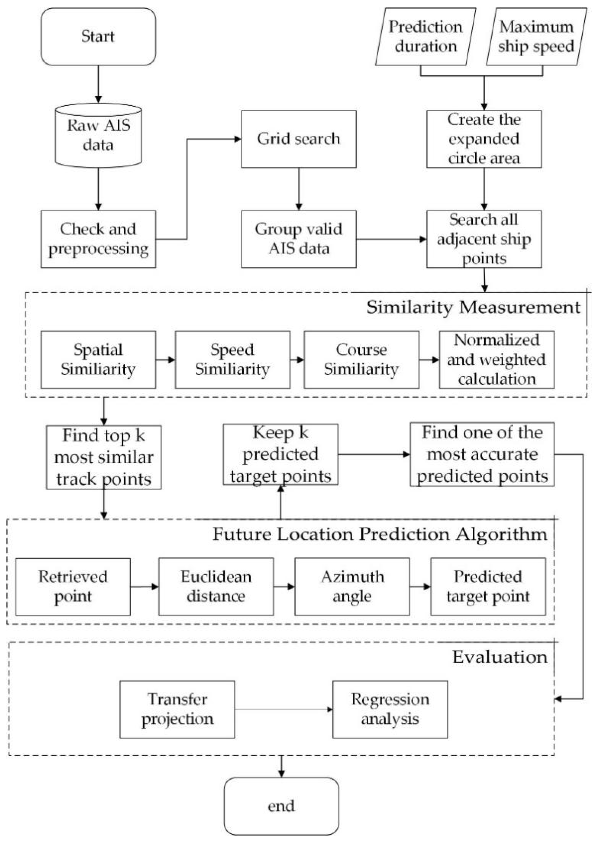
The method of short-term ship trajectory location prediction is illustrated in this section, as shown in Figure 1. We check and preprocess raw AIS data derived from constructed datasets. The method of the grid search is aimed at clearing some invalid points that the ship trajectory contains including stop action and hover behavior. After this step, valid AIS data are distinguished to constitute the ship trajectory. (2) The expanded circle area was created according to the prediction time and max speed of the ship. In combination with the two previous steps, relative ship points might be found in the above range. (3) All ship points are calculated to get their similarity value through similarity measurement. To get top k points similar to the target one, we derive the results according to similar values sorted in descending order. (4) The algorithm for future location prediction makes use of retrieving points from the trajectory that is preprocessed. By applying this k-nearest neighbor model to ships of similar property in the expanded circle area, we take an appropriate predicted point from traffic trajectory within the area. (5) The most accurate predicted point obtained is estimated to achieve final precision through the evaluation model.

Figure 1. Schematic of proposed ship location prediction flow.

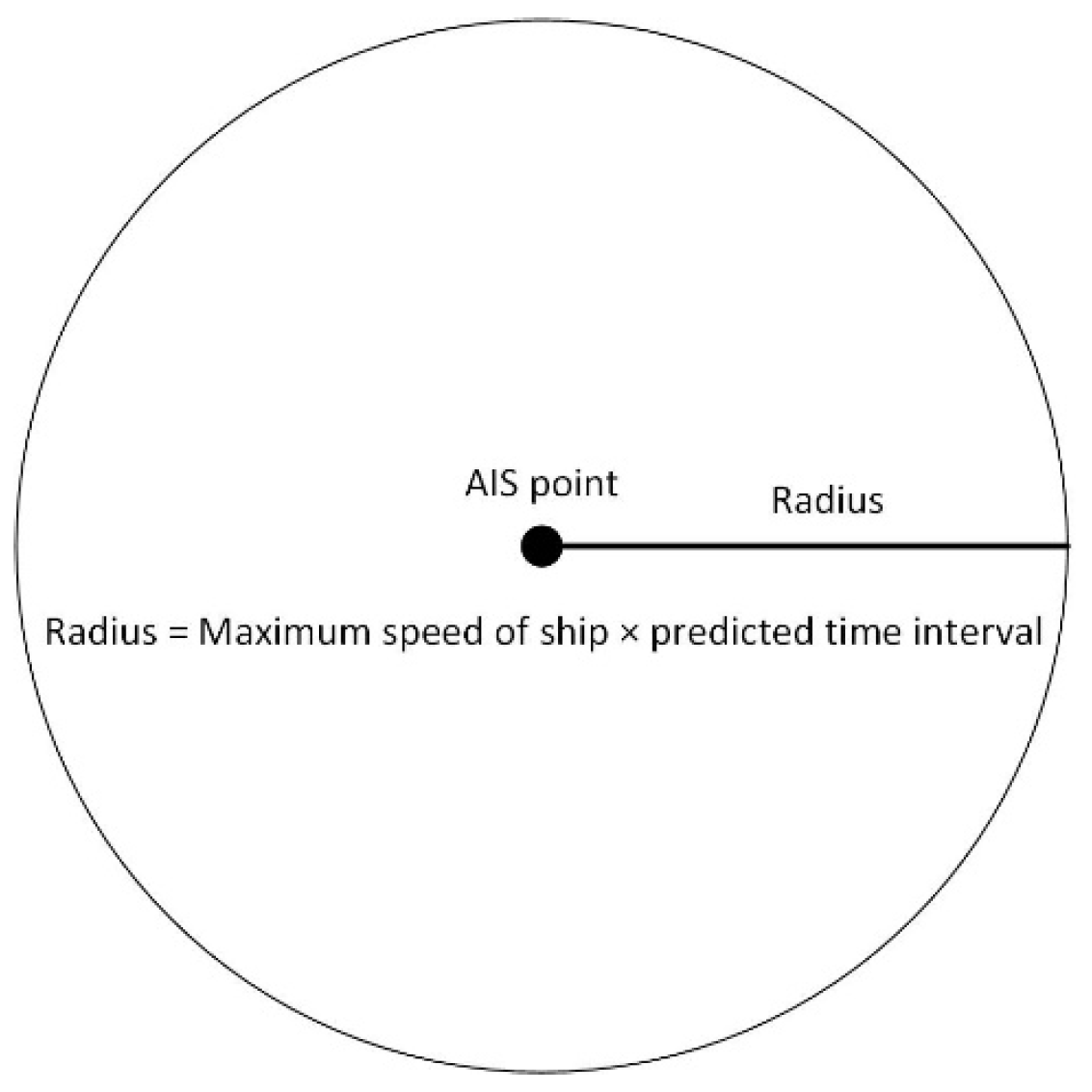
3.1. Expanded Area

To accurately predict the future trajectory location of a ship, a distribution of all possible locations should be predetermined. In this study, the concept of expanded area was defined as the maximum distribution range of the predicted trajectory location. The expanded area is a circular area around the last trajectory point of the target ship before location prediction. The size of the expanded area depends on the maximum speed of the target ship before location prediction and the specified predicted time interval. The centroid of the circular area is the last updated AIS point of the target ship before prediction, and its radius can be calculated by the product of the maximum speed over ground in the previous trajectory and the predicted time interval, as shown in Figure 2.

Figure 2. Expanded area.

The generated expanded area is mainly used to detect nearby trajectory points produced by other ships. Its range will be expanded by increasing the predicted time interval if there are no trajectory points detected. The time intervals usually range from 10 min to 30 min and the maximum speed of the ship is no more than 30 knots.

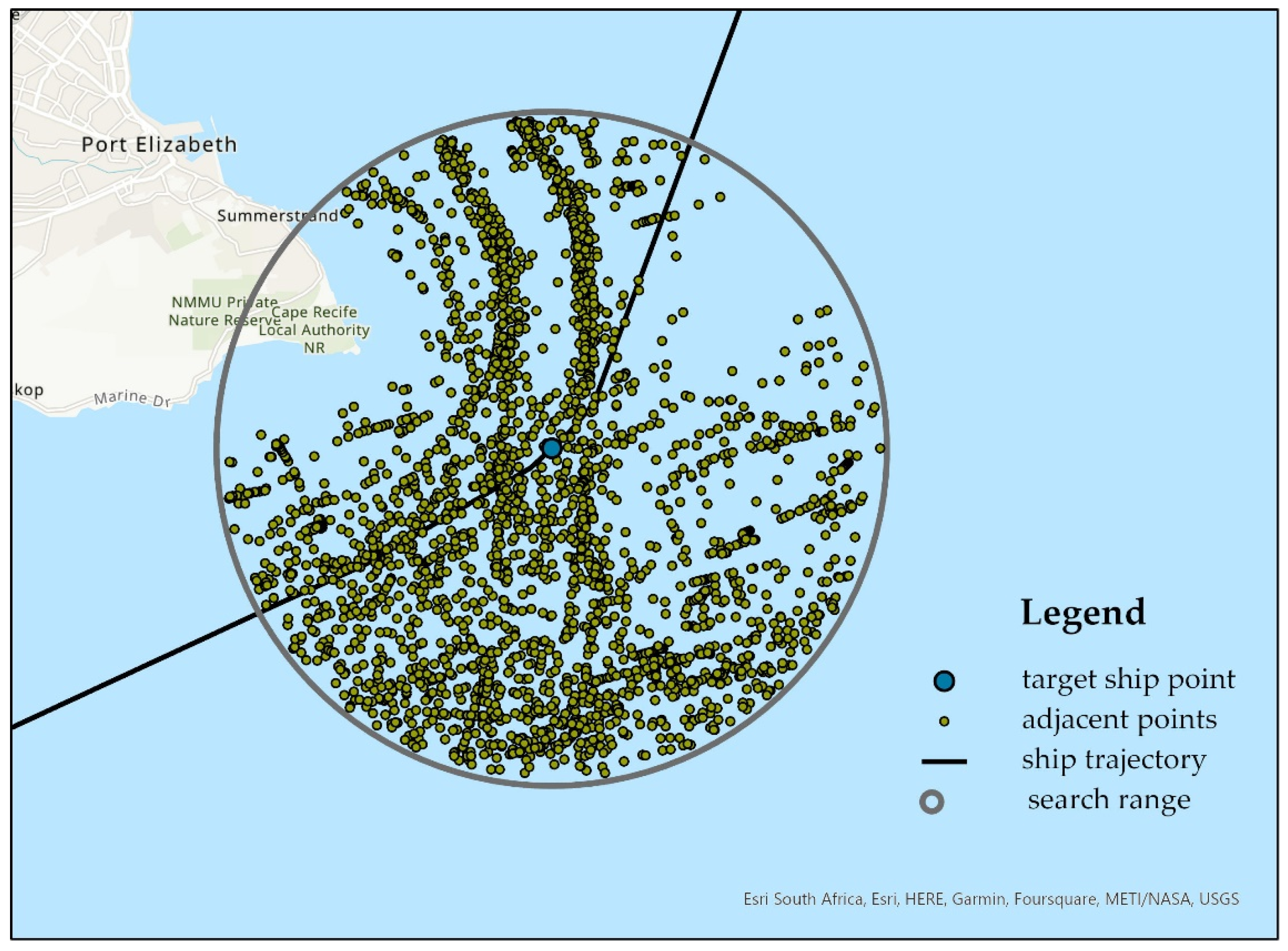
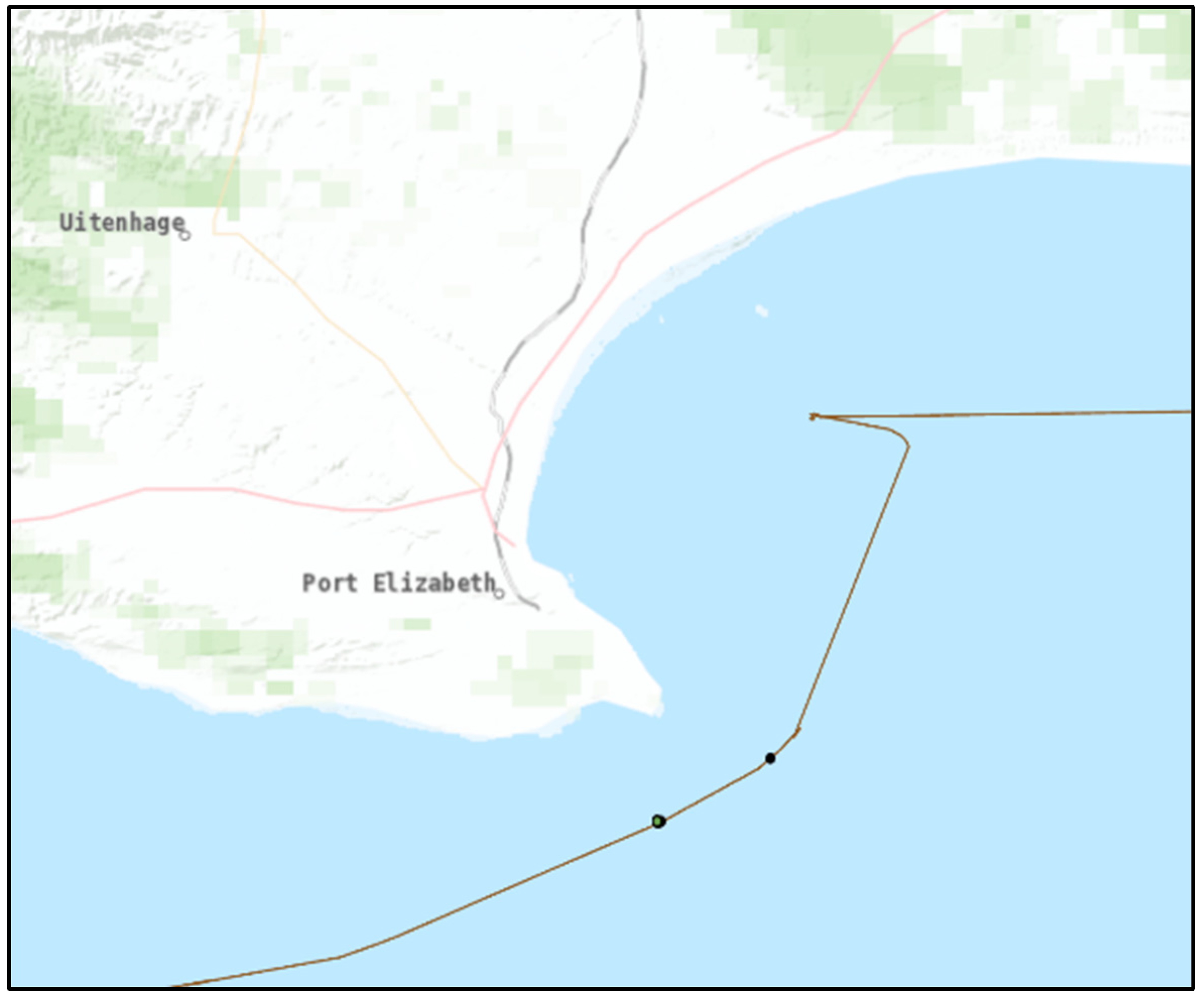
Figure 3 shows an example of searching nearby AIS points with the expanded area. The blue point represents the start point of the target ship before prediction. All trajectory points adjacent to the start points are extracted and shown as dark yellow dots. The Euclidean distance between these points and the start point is normally less than the radius of the expanded area.

Figure 3. Example of searching adjacent points in the expanded area for target ship.

3.2. Similarity Model

The distances between the points of the top trajectory to the corresponding points of the next trajectory are measured in terms of the trajectory similarity index [27]. The measurement of these points depends on the data and parameters of movement and static information such as coordinates, draught, ship type, heading, and environmental conditions. The most similar ship to the target ship based on the key status is chosen to predict the next location. The selected state for the similarity measurement shows the real process of navigation between the last place and the next place [28]. We obtain the information extraction from the AIS data. Spatial parameters, such as latitude and longitude, are identified as the main objects of the similarity model according to the first law of geography, which states that everything is related to everything else, but near things are more related than distant things, and the third law of geography, which explains that the more similar the geographic configurations of two points, the more similar the values of the target variable at these two points [29].

In the similarity model, we take into consideration three distance factors which are spatial distance, speed distance, and course distance.

Spatial distance is based on the Euclidean distance between the trajectory points of the target ship and the coordinates of the other vessels in the dataset. Euclidean distance is described according to the following equation:

$$D_s=\sqrt{{(x_t-x_d)}^2+{(y_t-y_d)}^2}$$

(1)

In the equation, $x_t$ and $y_t$ denote the coordinates of the target ship in the UTM projection system. $x_d$ and $y_d$ stand for the coordinates of trajectory points of other ships in the dataset. The spatial distance is given by $D_s$.

Speed distance is the absolute difference between the speed from the trajectory points of the target ship and speed from the trajectory points of other vessels in the dataset. The speed distance is defined according to the following equation:

$$D_v=\left|So{g}_t-So{g}_d\right|$$

(2)

In the equation, $So{g}_t$ denotes the speed of the trajectory point of the target ship before predicting the next location. $So{g}_d$ is the speed of the historical trajectory of other vessels. The speed distance is given by $D_v$.

Course distance is computed by using the absolute difference between the course from the trajectory points of the target ship and the course from the trajectory points of other vessels in the dataset. Cog is the property of AIS data, which depicts the real direction that ships have navigated. The course distance is defined according to the following equation:

$$D_c=\left|Co{g}_t-Co{g}_d\right|$$

(3)

In the equation, $Co{g}_t$ denotes the course of the previous trajectory point of the target ship when predicting the next location. $Co{g}_d$ is the course of the historical trajectory of other vessels. The course distance is given by $D_c$. Distance factors ($D_s$, $D_v$, $D_c$) are normalized to the value ranging from 0 to 1 according to the following equation:

$$D_n=\frac{D-Dmin}{Dmax-Dmin}$$

(4)

In the equation, the result of distance after normalization is given by $D_n$. $Dmax$ is the maximum value of distance and $Dmin$ is the minimum value of distance in the similarity measurement. As a consequence, the formula of the similarity measurement is combined with different distance measurements, which is defined according to the following equation:

$$D_{similar}=W_s\times D_{ns}+W_v\times D_{nv}+W_c\times D_{nc}$$

(5)

In the equation, $D_{ns}$, $D_{nv}$, and $D_{nc}$ denote the results of spatial distances, speed, and course based on normalization procedure. $W_s$, $W_v$, and $W_c$ stand for the weight of similarity variables. The accumulation of weights remains at the value of 1.

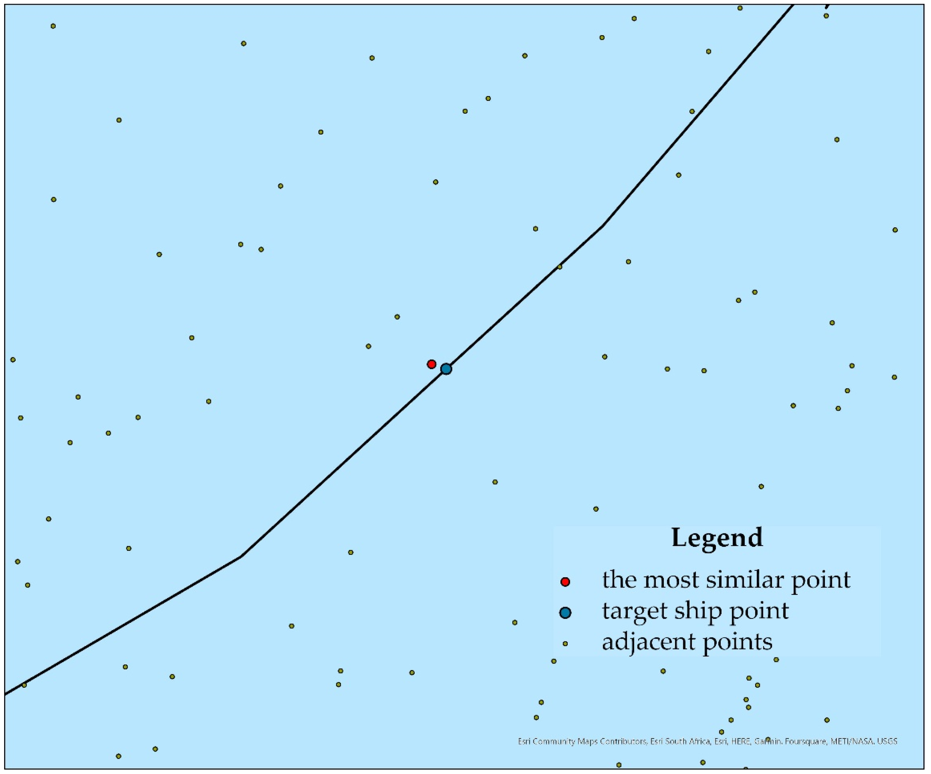
$D_{similar}$ represents the result integrated with the attributes of spatial distance, speed, and course variables from AIS datasets. The lower the value of $D_{similar}$, the higher the similarity between the target ship and the particular ship trajectory. An example of the most similar point retrieved is shown in Figure 4.

Figure 4. Example of the most similar point retrieved among similar points.

3.3. k-Nearest Neighbor Points Model

K-nearest neighbor (KNN) is an algorithm based on spatial or statistical classification and is a generalization of the nearest neighbor method. The input of the k-nearest neighbor method is the feature vector of the sample, which corresponds to the points in the feature space. The output is the category of test samples, and multiple categories can be selected. During classification decision making, the newly arrived sample points to be tested are predicted by a weight mechanism according to the category of K sample points of the k-nearest neighbor method. Therefore, the k-nearest neighbor method does not have an explicit learning process. It uses the dataset to divide the feature vector space and serve as its classification model. The results are classified by the similarity of sample vectors according to the following equation:

$$s_{\left(x_i,x_j\right)}=\sqrt{{\displaystyle \sum }_{k=1}^n{\left(x_{ik}-x_{jk}\right)}^2}$$

(6)

In the equation, the similarity between vector $x_i$ and vector $x_j$ is given by $S_{\left(x_i,x_j\right)}$, which is described by Euclidean distance. $k$ denotes the selected sample. $n$ is the number of samples.

In the first part of obtaining the top k most similar trajectory points, we calculate the coordinates of similar points relative to the ship trajectory point as a category. By identifying the number of similar points, the distance from them to the start point and their specific value towards similarity are considered through the KNN algorithm.

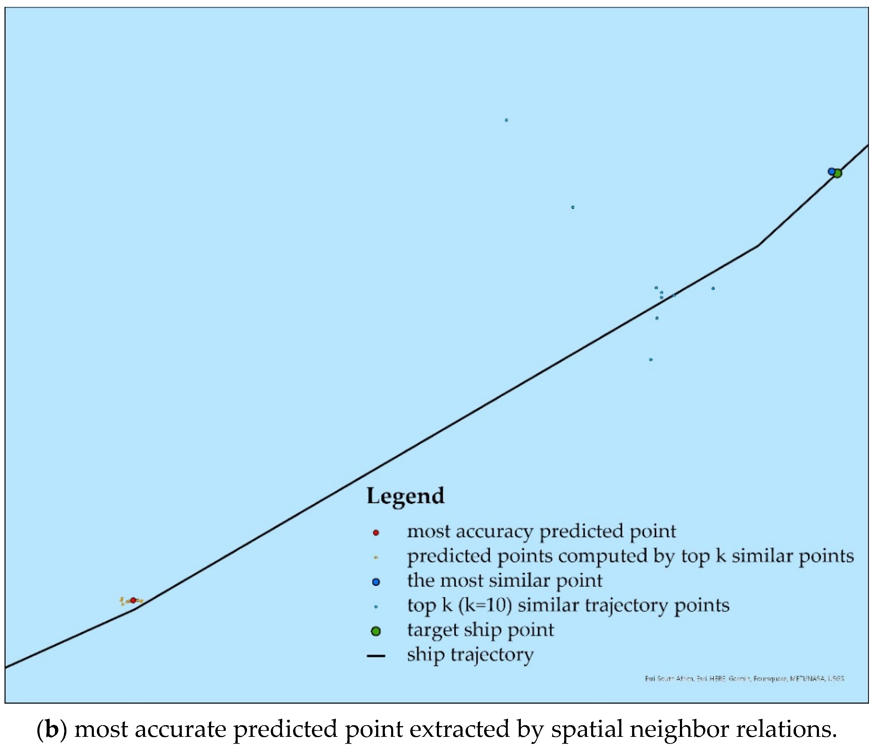
In the second part of obtaining the most accurate predicted point, we count the relative position from these predicted points to the actual trajectory. By using the operation of weighting and averaging the distance factors, these predicted points are computed to acquire the final point that is nearest to the location of the target ship.

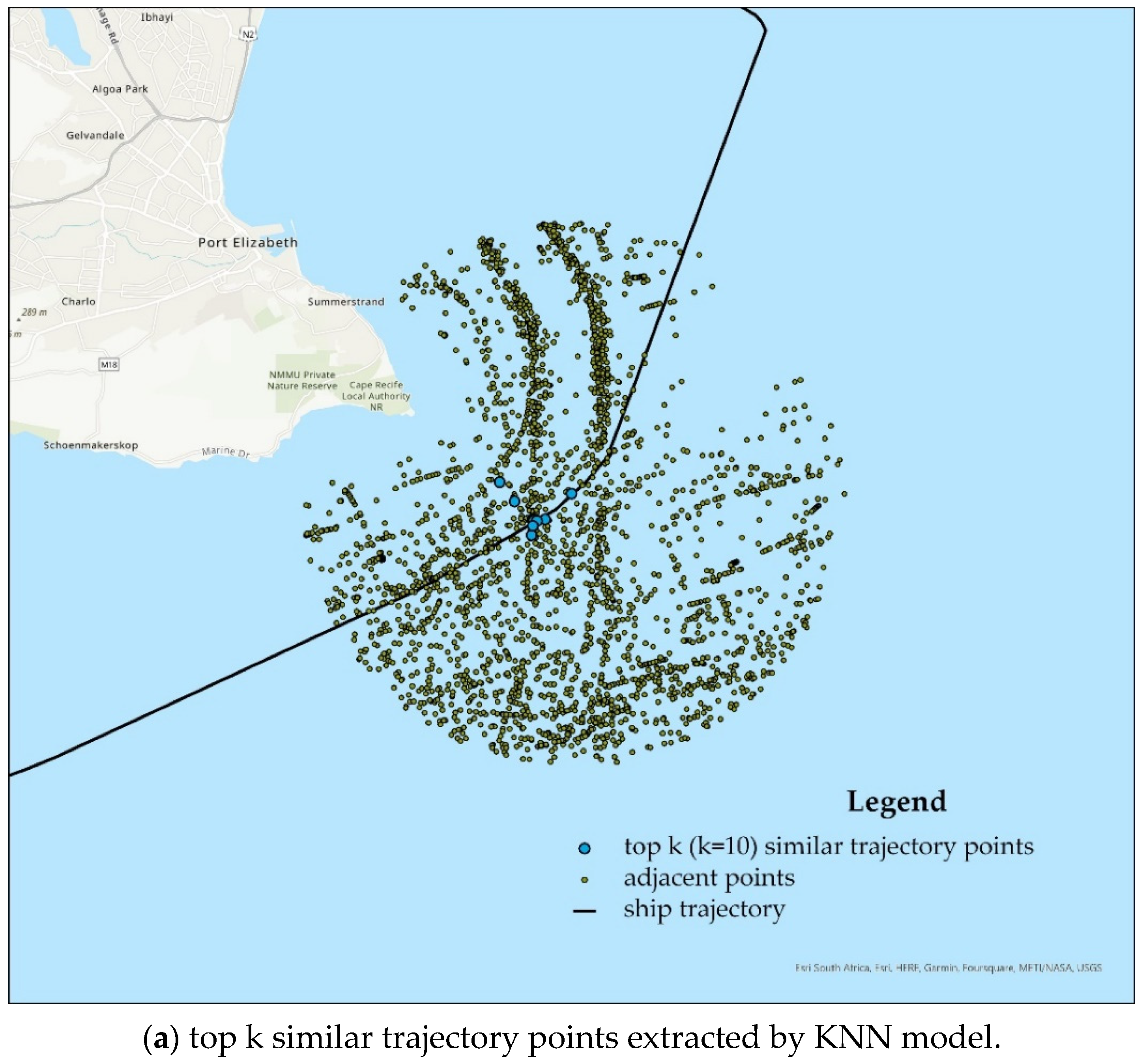
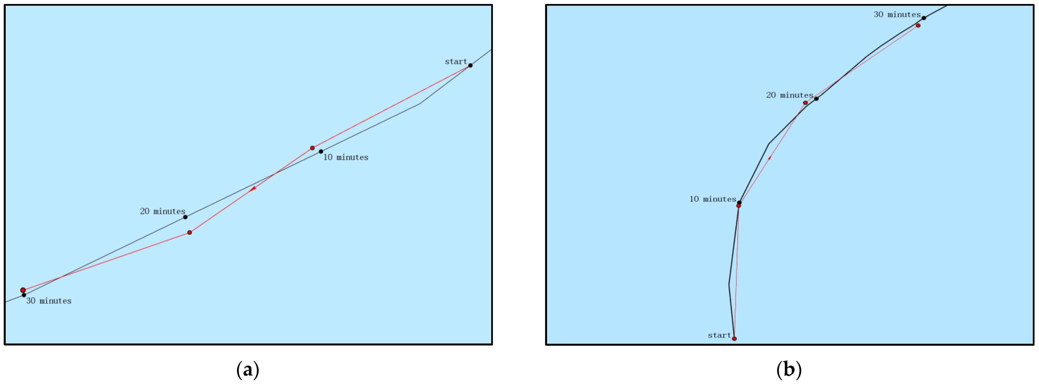
The top k (k = 10) similar trajectory points were extracted by the k-nearest neighbor points model, as shown in Figure 5a. The most accurate predicted point was extracted by spatial neighbor relations in the surroundings, as shown in Figure 5b.

Figure 5. Examples of results obtained by the KNN model.

3.4. Future Predicted Location Model

Ships navigate in a predetermined route which is based on their running status and destination. By analyzing the behavior of several ships similar to the target ship, the prediction of the target ship is determined by the use of semantic features such as similar ship trajectory.

The future predicted location model works as follows: (i) The ship most similar to the target ship is listed in the results of the similarity method. (ii) We calculate the distance between the point of the target ship and the point of the extracted ship according to Equation (1). (iii) We predict the next coordinate of the target ship by considering the trajectory of the extracted ship after computing the future path of the extracted ship within a time interval. It is also supposed that the distance between two points is constant.

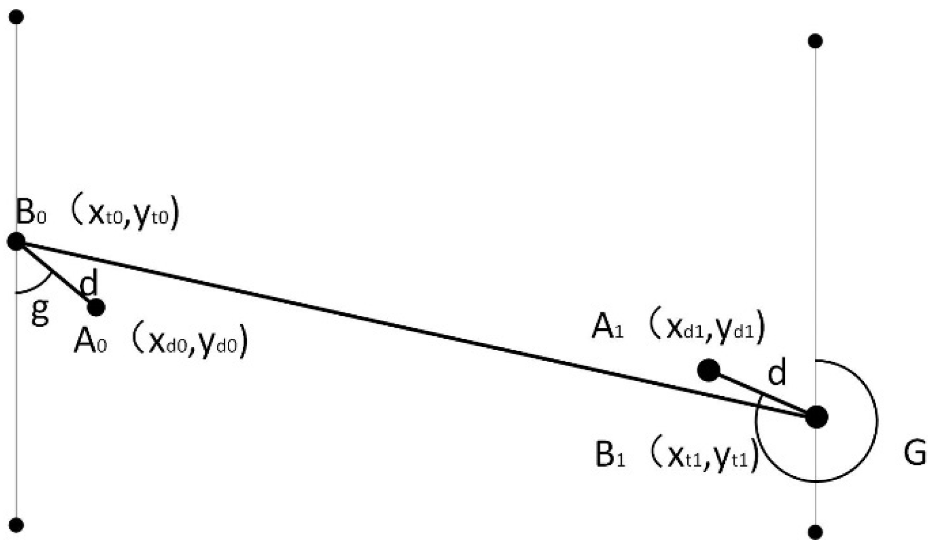
After retrieving the most similar ship trajectories from the dataset, the future coordinates of the target ship refer to the trajectory points of a similar vessel. The schematic of the prediction model is shown in Figure 6.

Figure 6. Future location prediction model.

In this figure, $A_0$ is the point of the target ship, and $B_0$ is the similar point of other ships after the results of the KNN model. Point $A_0$ links with point $B_0$ and the distance between two points is given by $d$. $A_1$ is the future point of the target ship compared to $B_1$ which is the next point of the extracted ship estimated by its navigation route in a time slice. $g_{B0A0}$ indicates the bearing angle which is based on points $A_0$ and $B_0$ according to the following equation:

$$g_{B0A0}={\tan }^{-1}\left|\frac{x_{t0}-x_{d0}}{y_{t0}-y_{d0}}\right|$$

(7)

In the equation, angle $g_{B0A0}$ is the angle with points $A_0$ and $B_0$. ($x_{d0}$,$y_{d0}$) is the coordinate of point $A_0$ and ($x_{t0}$,$y_{t0}$) is the coordinate of point $B_0$ at time $t0$. $G$ is the azimuth angle depicting the direction of north, which is defined according to the following equation:

$$G_{B0A0}=\{\begin{array}{c}{g}_{B0A0}\\ 180-g_{B0A0}\\ 360-g_{B0A0}\\ 180+g_{B0A0}\end{array}$$

(8)

In the equation, the angle $G_{B0A0}$ is the angle that is directed to $B0A0$ at time $t0$. It is assumed that $G$ and d remain constant for the prediction duration when $d$ and $G$ are completing computing until the next coordinate of the target ship has been predicted. The predicted location of the target ship at time $t1$ is defined according to the following equation:

$$\begin{array}{l}{x}_{d1}=x_{t1}+d\times \sin G_{B0A0}\\ y_{d1}=y_{t1}+d\times \cos G_{B0A0}\end{array}$$

(9)

In the equation, coordinate ($x_{d1}$,$y_{d1}$) stands for the coordinate of the future location of the target ship. ($x_{t1}$,$y_{t1}$) represents the coordinate of the location of the extracted ship at time $t1$. The value of $G_{B1A1}$ is the same as the value of $G_{B0A0}$. The spatial distance is given by $d$.

Predicted points result from the number and coordinate of similar points. An example of the results of predicted points obtained is shown in Figure 7.

Figure 7. Examples of results of predicted points.

4. Analysis and Evaluation

4.1. Case Study

The AIS dataset was collected in the water of South Africa from March 2020 to April 2020, as shown in Figure 8. The spatial range of the dataset is from 2,800,000 m to 3,200,000 m in the horizontal direction and from −4,300,000 m to −3,800,000 m in the vertical direction in the Web Mercator coordinate system.

Figure 8. Study area: water of South Africa.

4.2. Data Preprocess

The dataset contains a total of 146,346 ship trajectories consisting of 29,197,704 sampling points. The trajectories with zero speed indicating ship stay were first filtered from the dataset since ships that remain stationary are not valuable reference objects. The following step was loitering behavior detection of ship trajectories. Many vessels may perform loitering movements when they conduct offshore operations, fishing, surveys, search and rescue, and other activities. The shapes of loitering movements are usually similar to ellipses, round-trip polylines, random coils, and sigmoid curves. Such trajectories cannot be used for location prediction either and were removed from the dataset using the method proposed by Huang et al. [30]. Then, the experiment procedure is as follows: (i) Take a location point of the ship as a target randomly. (ii) Search the trajectory points of other ships in the expanded range. (iii) Calculate the similarity index of ship trajectory points in the range. (iv) Calculate the top k similar points. (v) Calculate the future location of the target ship at 10 min, 20 min, and 30 min according to top k similar points. (vi) Complete the above steps a number of times based on different ship trajectory samplings.

4.3. Result

Figure 9 shows a case of comparison between the actual points and the predicted points of the target ship in two different movements. The black polyline represents the original trajectory of the target ship, and the red polyline is the predicted trajectory in contrast. The arrow of the polyline points out the sail direction of a vessel. For both straight and turning movements, three prediction points within 10 min, 20 min, and 30 min are generated based on the start point. It can be observed that the predicted trajectory has a similar movement to the actual trajectory in the zoomed-in images. Detailed coordinates of each pair of the actual point and the predicted point are listed in Table 2. The position deviation between each pair of points is small.

Figure 9. Comparison of actual points and predicted points with a 10 min prediction time interval. (a) Straight movement; (b) turning movement.

Table 2. Example values of time duration, ActualLongitude, ActualLatitude, PredictedLongitude, and PredictedLatitude.

Duration	ActualLongitude	ActualLatitude	PredictedLongitude	PredictedLatitude
10 min	25.752386	−34.075121	25.751002	−34.074525
20 min	25.73014	−34.085871	25.73086	−34.088417
30 min	25.703685	−34.098655	25.703518	−34.097876

4.4. Evaluation

The output results were separated into many groups before further precision evaluation. The size of each group varies from 10 to 50. Each result in the group is represented as a vector consisting of a pair of the actual location coordinates (actualX, actualY) and predicted location coordinates (predictedX, predictedY). To better evaluate the prediction precision, all longitude and latitude coordinates of actual locations and predicted locations in the WGS84 spherical coordinate system are converted to plane cartesian coordinates in the UTM project coordinate system. Table 3 shows some examples of transformed coordinate values of actual location and predicted location.

Table 3. Examples of transformed values of actualX, predictedX, actualY, and predictedY.

n	ActualX	PredictedX	ActualY	PredictedY
1	2,945,636	2,946,988	−4,070,922	−4,070,315
2	2,945,626	2,947,540	−4,007,540	−4,008,923
3	2,945,576	2,945,548	−4,066,246	−4,069,241
4	2,945,407	2,932,752	−4,075,356	−4,071,241
5	2,945,347	2,945,116	−4,033,137	−4,034,750

The linear regression model is then used to analyze the correlations between the actual points and the predicted points. The least squares linear regression is applied to determine the essential parameters of the linear equation, $y=mx+b$, by minimizing the error of the square of the difference between y and its estimation value.

$$E={\left(y-m\times x-b\right)}^2$$

(10)

The scatter plot with $R^2$ values is used to show the degree of approximation between predicted coordinates and actual coordinates, as illustrated in Figure 10. In this case, we compute the parameter $R^2$ for the $X$ and $Y$ values. The value of $R^2$ ranges from 0 to 1. The value 1 means the predicted values are the same as the actual values. However, 0 means that the actual values and predicted values are irrelevant.

Figure 10. Scatter estimation plot between actual and predicted values (a,b) show the correlation of X and Y within 10 min; (c,d) show the correlation of X and Y within 20 min; and (e,f) show the correlation of X and Y within 30 min.

In each chart of Figure 10, the actual and predicted values are presented on the horizontal and vertical axes. The line drawn on the diagonal indicates that $Y$ values are equal to $X$ values. Points observed closer to the plotted line represent higher accuracy of the predicted results. The correlation in $Y$ is better than that in $X$.

The similarity measurement [8] is compared with our proposed method in Table 4. The values of $R^2$ are calculated in each method. Table 4 shows the ultimate precision results and indicates that as time duration increases, $R^2$ decreases dramatically.

Table 4. The values of R² to X, Y, or XY merged by evaluation in different durations.

Method	Duration	R2 (X)	R2 (Y)	R2 (XY)
KNN	10 min	0.990	0.994	0.992
	20 min	0.988	0.992	0.990
	30 min	0.986	0.989	0.9875
Similarity measurement	10 min	0.962	0.974	0.968
	20 min	0.947	0.956	0.9515
	30 min	0.909	0.923	0.916

It can be seen from the table that the KNN method has higher $R^2$ values and better prediction accuracy than the similarity measurement. The task of short-term trajectory prediction of maritime vessels will be carried out better by using the KNN algorithm. This also shows that the KNN algorithm has the advantage that the optimal result can be obtained from the sample data. However, due to the factor of geographic location, the trajectory point of the target ship near the port has relatively more adjacent sampling points than the trajectory points of other water locations, which may lead to low-precision results of prediction in locations other than the area of the port. Moreover, the mean error is not suitable for this evaluation of the results because a marginal case of prediction result affects the accuracy dramatically.

5. Conclusions

This study aimed to use a multi-algorithm combined model based on motion parameters obtained from AIS data for predicting vessel locations. In this study, the innovation was to use the KNN method to improve the methods and precision. The results of the predictions are derived from the predicted points of ships within the time range of short-term prediction. The expanded circle area is designed according to the max speed of the ships and the duration of the prediction. The effect of the prediction result is the best at the beginning, but prediction error rises as duration increases.

Although ship location recognition in a short time works with the model, it was assumed that the factors of the target ship and the similar ships retrieved in the KNN method were simple, so it is not applicable to long-term prediction. Moreover, the weight of the parameters is not dynamic in the similarity model.

In future studies, we suggest executing measures based on trajectory classification with long-distance and short-distance vessels to predict within the defined range and evaluating the prediction errors with MAE and RMSE. The contributing factors of the environment of the sea combined with the AIS data should also be taken into account in the prediction of ship movement.