Advantage of Regional Algorithms for the Chlorophyll-a Concentration Retrieval from In Situ Optical Measurements in the Kara Sea

Abstract

The data of the sea reflectance coefficient were obtained during the cruise of the R/V “Akademik Ioffe” (10 August–8 September 2021) in the Kara Sea beyond the Arctic Circle. A total of 28 measurements of sea reflectance were performed in different conditions ranging from estuarine zones to open ocean. In addition, at 10 stations, water samples were taken, and chlorophyll-a concentrations were determined using the fluorometric method. In situ reflectance data were compared to satellite data (MODIS Aqua/Terra, Sentinel OLCI 3A/B, VIIRS SNPP) obtained within 24 h before and after the measurement. It was shown that, in general, an overestimation of remote sensing reflectance is observed in short-wave channels (412, 443, 469 nm for MODIS; 410, 412.5, 442.5 for OLCI) and underestimation in long-wave channels (708.75, 753.75 nm for OLCI). The obtained in situ chlorophyll-a concentrations were compared with the results of standard models (GIOP, OC2, OC3, OC4), and regional algorithms (semi-analytical MHI, empirical K17) were applied to the in situ and remotely sensed reflectances. In the cases of GIOP and OC4, unrealistic concentrations of chlorophyll-a were obtained. Regional algorithms developed earlier, specifically for the Kara Sea, showed good correlation (0.6 and 0.76) with in situ measurements. Despite the approximately 20% overestimation of chlorophyll-a by both regional algorithms, they can be used to obtain chlorophyll-a concentrations in the Kara Sea in a concentration range of <1 mg/m³.

1. Introduction

Chlorophyll-a concentration is one of the most important marine ecosystem parameters available from satellite imagery. It is widely used to calculate the primary production [1] or the radiation balance [2,3] of the ocean. It can also serve as a contrast substance allowing for the study of ocean dynamics, such as manifestations of surface currents, eddies, and frontal features [4]. However, the algorithms for obtaining chlorophyll-a concentrations from satellite data do not always take into account regional features, such as rivers bringing suspended sediments and increasing water productivity [5,6]. The influence of river runoff or melting of ice can change seawater composition, affecting the inherent hydro-optical characteristics and the distribution of chlorophyll-a in the surface water layer [7,8,9]. All this leads to the incorrect performance of satellite algorithms [10]. One way to solve this problem is to create regional algorithms based on the local datasets, inherently taking into account the characteristic features of the studied region [10,11]. The presented work discusses various types of algorithms developed earlier [5,6,12] that allow obtaining the chlorophyll-a concentration in the Kara Sea, based on satellite and in situ remote sensing reflectance.

The Kara Sea is an interesting object for study due to the strong anthropogenic influence. A part of the Northern Sea Route lies in the Kara Sea, and it is subject to intensive fishery [13]. Rapid development of the Arctic region leads to the increase in pressure on the ecosystem. Monitoring the ecological state of the region can be performed using one of the key parameters, i.e., chlorophyll-a concentration.

The Kara Sea belongs to the case 2 waters [14,15]. The characteristic feature of the Kara Sea is the significant influence of the river runoff on the upper layer [16,17]. The desalinated layer has its distinctive optical properties caused by the high colored dissolved organic matter (CDOM) content, suspended particles, and marine and possibly river phytoplankton in the water [18]. All these parameters can be obtained from satellite data, but standard algorithms do not take into account the regional features of the Kara Sea. For example, overestimated values of chlorophyll-a concentration appear in the desalinated layer due to the significant content of CDOM that entered the sea with the river flow [19]. The algorithms, for instance, ocean color, which uses 4 channels (OC4) [6,20], are designed for case 1 waters, so they partly describe CDOM absorption as an absorption due to chlorophyll-a. However, the satellite products qualitatively reflect the important features of the chlorophyll-a spatial distribution, such as high values of chlorophyll-a concentration observed near Ob Bay and Yenisei Bay and low values in the northeastern part of the Kara Sea [12].

To achieve more accurate values of chlorophyll-a concentration, the regional algorithms are developed based on the in situ data of the sea reflectance obtained by contact measurements. In order to design, validate, and check the regional bio-optical models, the data of direct chlorophyll-a measurements in samples are utilized.

Due to frequent cloudiness over the Kara Sea region, it is difficult to obtain satellite images synchronous with in situ measurements. Average cloud cover from June to October is 80–90% [12]. Therefore, satellite data from all available ocean color scanners were used whenever possible. OLCI, MODIS, and VIIRS have many bands across the visible spectral range, which allow utilizing them for calculations using regional algorithms. Landsat could not be used for this purpose due to the width between the channels.

Another difficulty of remote estimation of chlorophyll-a concentration in the Arctic region is the atmospheric correction. Usually, atmospheric correction algorithms are based on a plane-parallel radiative transfer assumption [21], which is valid for the Sun zenith angles <70°. At high latitudes, the Sun zenith angle during the measurements is often larger than 70°. The presence of ice, clouds, and fog not only cover significant areas from view, but could also produce an adjacency effect, contaminating the retrieved seawater reflectance [22,23]. However, to what extent the abovementioned conditions compromise the use of ocean color sensors in polar areas is yet unknown.

The standard atmospheric correction algorithm has the only flexibility: to tune its aerosol model to fit the measurements. The solution is to implement an Arctic aerosol model [24] or to use a more flexible atmospheric correction algorithm, such as POLYMER (POLYnomial-based approach established for the atmospheric correction of MERIS data), which does not use a specific aerosol model [25,26]. Another way is to introduce an additional correction parameterizing the properties of the seawater, as it was made, for example, in works [27,28].

The main aim of this work is to present in situ data of sea reflectance during the 2021 summer–autumn season for the Kara Sea and to compare them to satellite data in order to show the performance of the atmospheric correction for polar areas. Adaptation and further development of regional algorithms can significantly improve retrieval of the chlorophyll-a concentration in the Kara Sea. The application of two such algorithms is demonstrated in this paper (one empirical and one semi-analytical).

2. Materials and Methods

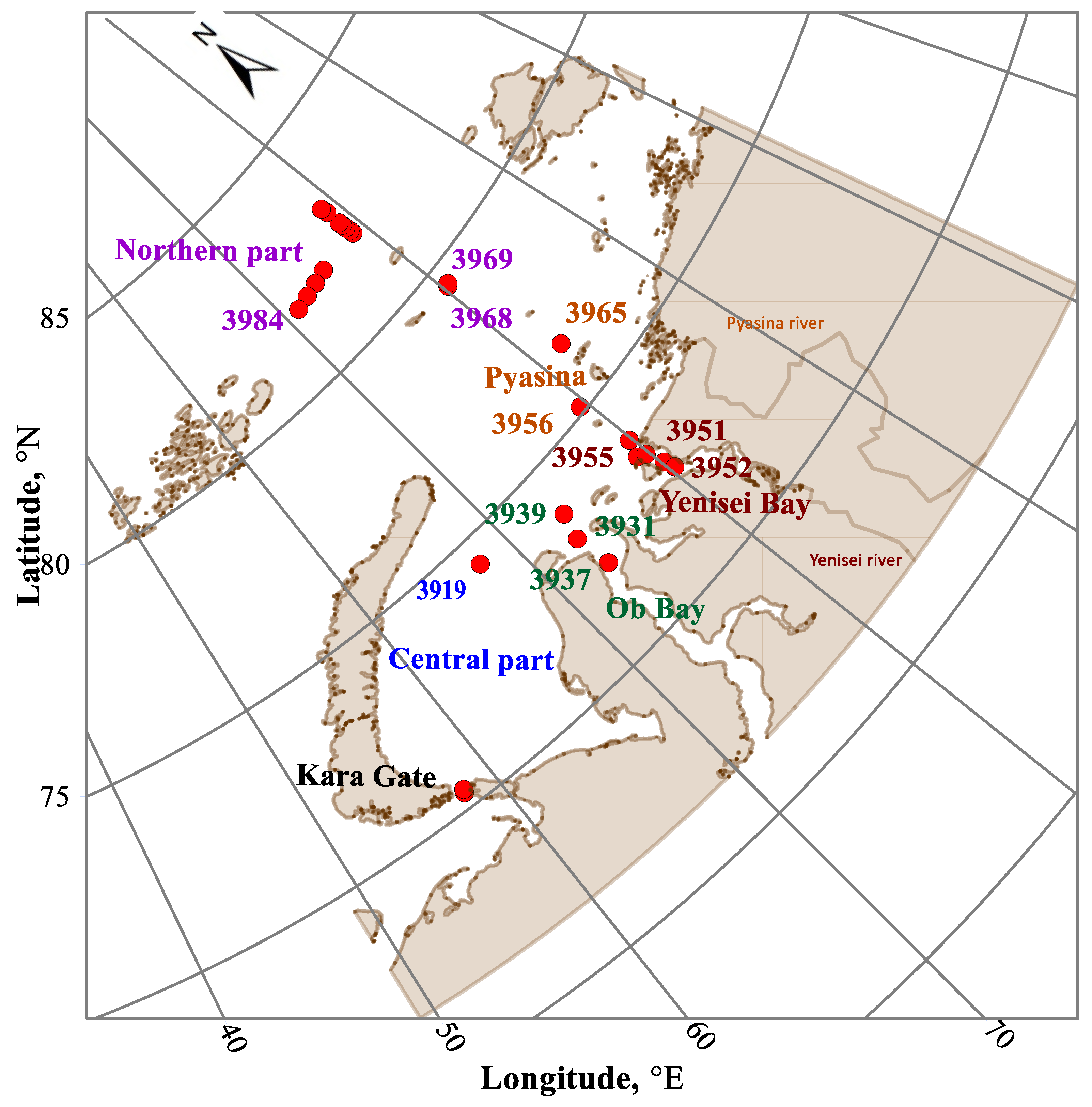
2.1. Study Area

The data were obtained during the 58th cruise of R/V “Akademik Ioffe” (10 August–8 September 2021). The study area in the Kara Sea was divided in 6 parts: the Kara Gates Strait, the central part, the northern part, and the estuarine zones of the Ob, Yenisei, and Pyasina rivers (Figure 1), in order to research separately the characteristics of the reflectance and the chlorophyll-a concentration, according to in situ and remote sensing measurements. The data for the northern part (north of 82° N) can be considered unique as this part of the sea is usually covered with ice. Stations of the optical measurements and sampling for chlorophyll are shown in Figure 1. Stations of chlorophyll-a sampling are marked with the color corresponding to a certain part of the sea.

2.2. Field Measurements

The main obstacles to carry out the experiments were frequent clouds, fog (high humidity), and low sun. In addition, the whitecaps, as a result of significant waves and floating ice, required the collection of continuous optical measurements in order to take time-averaged results and to therefore increase their quality. Hyperspectral upwelling radiation measurements were performed at each station with passable weather conditions (no fog, constant illumination conditions). At certain stations, samples for chlorophyll-a determination were taken from the surface layer (0–5 m).

Table 1. Study areas and corresponding numbers of in situ and remote sensing measurements.

Study Area	In Situ		Satellite Rrs
	Rrs	Chl	MODIS A/T	VIIRS SNPP	OLCI S3A/B
Kara Gates	2	-	-	-	-
Central part	3	-	4	1	1
Ob Bay	3	3	1	1	2
Yenisei Bay	5	3	2	1	4
Pyasina Bay	2	2	1	1	5
Northern part	13	2	-	-	6

shows the amount of data available for each part of the study area.

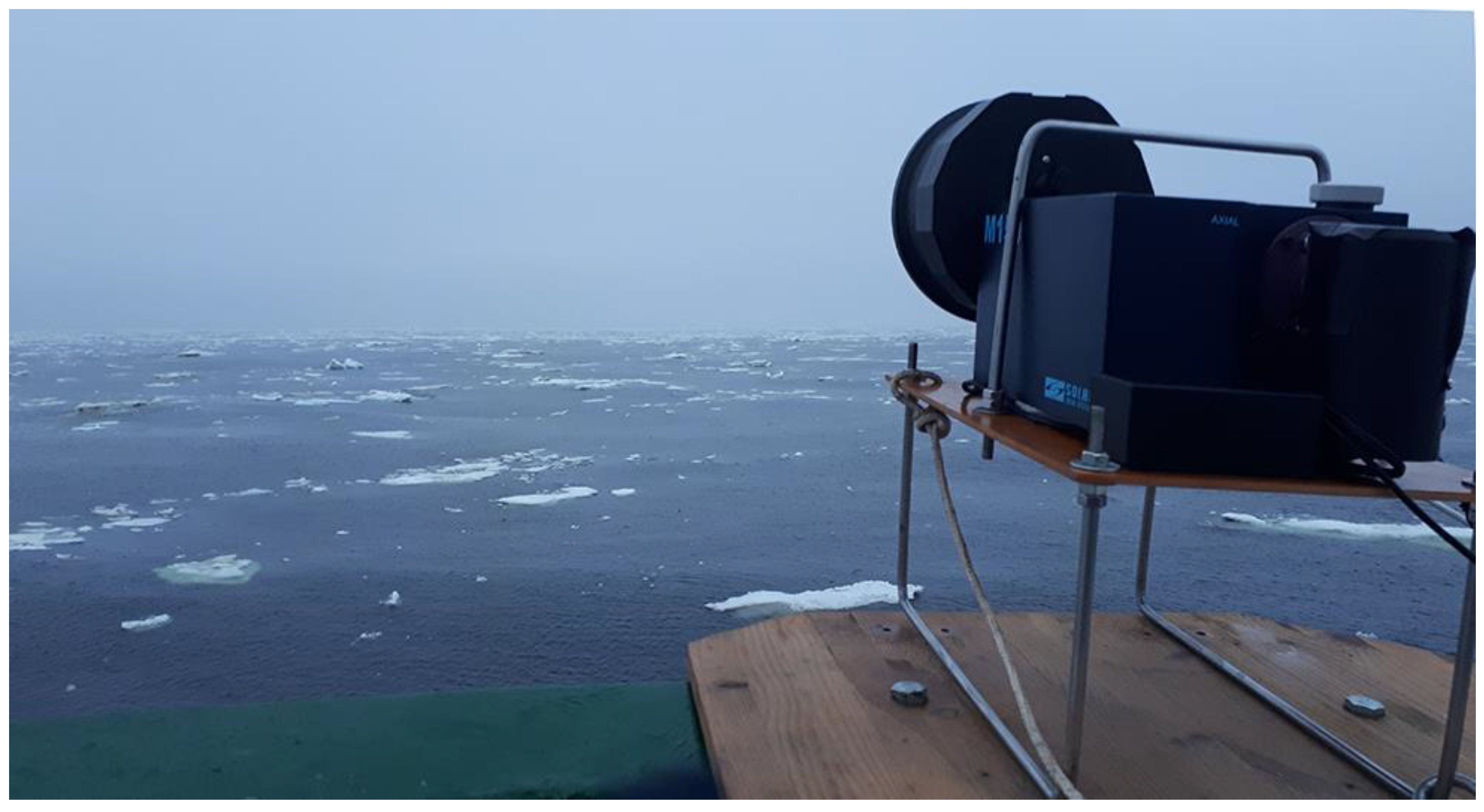
2.2.1. Upwelling Radiation Hyperspectral Measurements

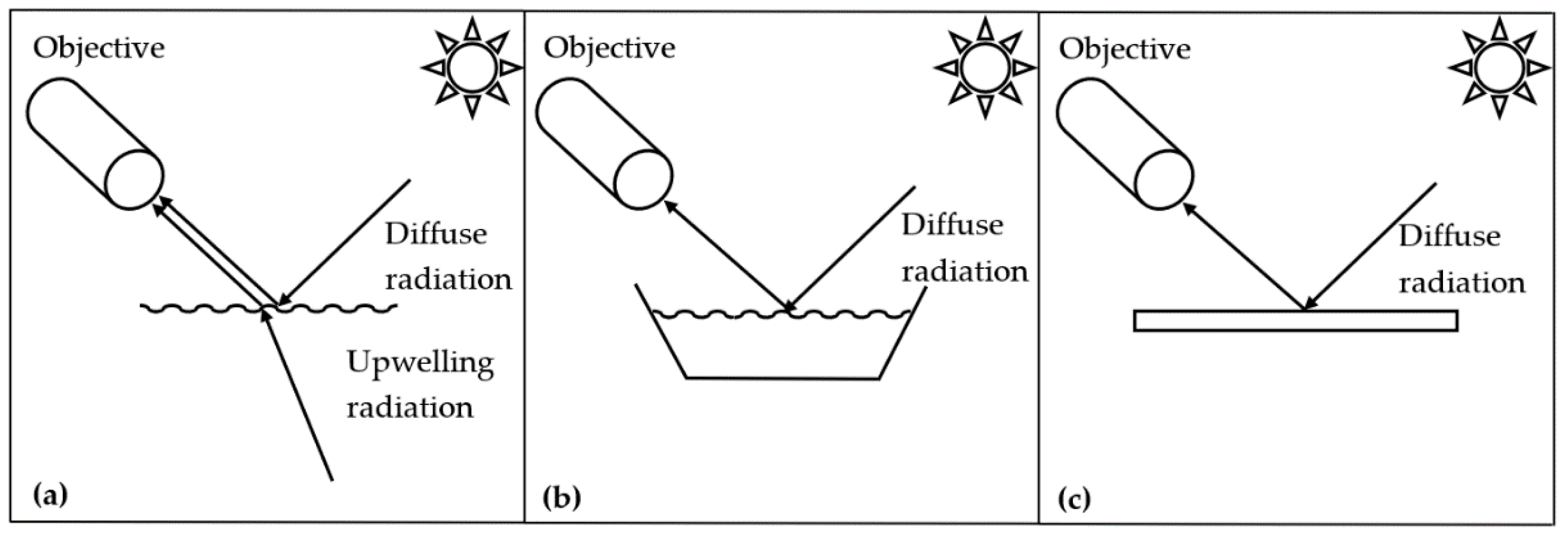
In order to obtain sea reflectance from above-surface measurements, it is usually necessary to measure the upwelling radiance $L_u$ and the radiance of the sky reflected by the water surface $L_{sky}$, as well as the downwelling irradiance E_d [29]. The water-leaving radiance is the difference $L_u-L_{sky}$, sea reflectance is defined as

$$Rrs=\frac{L_u-L_{sky}}{E_d}$$

(1)

In this study, a single spectrometer was used for all three measurements, as described in [30]. The spectrometer was designed in the Marine Hydrophysical Institute (MHI) based on Solar Laser Systems’ (www.solarlaser.com, accessed on 26 August 2022) monochromator M150. Remote sensing reflectance (Rrs) was measured from the board of the vessel in the spectral range 370–750 nm with 5 nm resolution. Measurement error was 1–3%. The sensor was placed about 5 m above water surface, pointing at 30° to nadir (Figure 2). The measurement process consisted in three measurements:

-

the total upwelling radiance $L_u$ from the sea surface (Figure 3a);

-

the radiance reflected from water surface $L_{sky}$, in the cuvette with walls and bottom made of dark neutral glass TC-3 [31] with absorption >99% in the visible range. Dimensions of the cuvette are 100 × 100 × 250 mm. The cuvette has a layer of water about 5 cm, so the water leaving radiance of the cuvette was negligible (Figure 3b);

-

the radiance of the horizontal white Lambertian panel $L_L$. with known reflection coefficient $R_L$, giving the downwelling irradiance $E_d=\pi L_L/R_L$ (Figure 3c).

The three measurements were performed within ~20 min. To compensate for the unsatisfactory weather conditions (waves, clouds), each quantity was measured for ~5 min, the obtained spectra were averaged, and then smoothed by the median filter. This method is consistent with NASA protocols [32].

The proposed method was used in sea expeditions [30,33,34] (Figure 3a) or from a stationary oceanographic platform [35]. The obtained spectra will be further denoted as in situ spectra.

2.2.2. Chlorophyll-a Concentration Measurements

The concentration of chlorophyll-a (Chl) in seawater samples was determined by the fluorometric method [36] using a Trilogy Turner Designs fluorimeter (Turner Designs, Inc., San Jose, CA, USA). The fluorimeter was calibrated using a chlorophyll standard manufactured by Sigma Chemical Co. (Sigma-Aldrich, Inc., St. Louis, MO, USA). Water samples (0.5 L) were filtered through Whatman GF/F fiberglass filters with the vacuum not exceeding 0.3 atm. Then, the filters were placed in a 90% acetone solution for the extraction of chlorophyll-a. The samples were kept in the dark for 24 h at a temperature of 4 °C. The fluorescence of the extracts was measured before and after acidification of 1 M HCl to correct the concentration of chlorophyll-a, taking into account pheophytin. The calculation of the concentration of chlorophyll-a and pheophytin, according to fluorescence data, was carried out according to the standard method [37].

Since the samples were taken at irregular horizons different for each station, only the surface concentrations were used in this study to compare with model data. In total, 10 stations were performed simultaneously with optical measurements and used in this study (Table 1).

2.3. Satellite Data

Satellite data from MODIS (Moderate Resolution Imaging Spectroradiometer) on Aqua (A) and Terra (T) satellites, VIIRS (Visible and Infrared Imaging Radiometer Suite) on Suomi NPP, OLCI (Ocean and Land Color Instrument) on Sentinel 3A and S3B Level 2 were used in this study, downloaded from Oceancolor Web and Copernicus websites [38,39]. MODIS radiometer provides Rrs in sr⁻¹ for 10 spectral bands: 412, 443, 469, 488, 531, 547, 555, 645, 667, and 678 nm. All bands were rescaled to 1 km spatial resolution. VIIRS provides Rrs at 410, 443, 486, 551, and 671 nm with the spatial resolution 750 m. OLCI radiometer provides dimensionless Rrs for 12 spectral bands: 410, 412.5, 442.5, 490, 510, 560, 620, 665, 673.75, 681.25, 708.75, and 753.75 nm, at full spatial resolution 300 m. OLCI Rrs were divided by π sr to compare with other satellite data. Chlorophyll-a concentrations from standard satellite products for the same three sensors were also used.

Due to the peculiarities of the Arctic region, such as frequent clouds, low sun, and ice cover, it is difficult to obtain a large amount of data that can be processed. Therefore, a necessary step to increase the set of satellite images for further analysis is to expand the time range between contact and remote measurements from 3 to 24 h [40]. The time and coordinates of satellite acquisition coincided with the time and coordinates of field measurements within 24 h and 1 km. Data were selected using the Seatrue feature of the SMCS software [41] and processed using SNAP package. Only the pixels with no clouds, ice, and stray light flags for MODIS and VIIRS and no clouds, ice flags and doubtful pixels for OLCI were considered. The amount of data is shown in Table 1.

2.4. Bio-Optical Algorithms

In this study we used the following models to evaluate the chlorophyll-a concentration: Generalized Inherent Optical Property (GIOP) [5] model, estimation from OC4v.6, as well as the OC2 and OC3 SeaWiFS [20] algorithm, regional empirical algorithm Kara Sea 2017 (K17) developed in the Laboratory of Ocean Optics of the Institute of Oceanology RAS [14], and semi-analytical algorithm developed in the Marine Hydrophysical Institute RAS (MHI) [34]. The reason for using OC4 and GIOP algorithms is that they are included in the standard NASA satellite Level 2 products and used most frequently in the marine bio-optical research.

Standard band ratio algorithm OCx [20] is based on a complex fourth-order polynomial dependence, which connects the values of the Rrs with the concentration of chlorophyll-a. OC2 uses 2 channels (“blue” 490 and “green” 555 nm) for OC3 and OC4 algorithms; the idea is that among the 2 or 3 values of the Rrs corresponding to the “blue” channels, the one with maximal Rrs is selected and used:

$${log}_{10}\left(Chl\right)=a_0+{\displaystyle \sum }_{i=1}^4{a}_i{\left({log}_{10}\left(\frac{R_{rs}\left({\lambda }_{blue}\right)}{R_{rs}\left({\lambda }_{green}\right)}\right)\right)}^i,$$

(2)

where $a_i$ are the empirical coefficients for the used sensor, ${\lambda }_{blue}$ = {443, 490} nm for OC3, ${\lambda }_{blue}$ = {443, 490, 510} nm for OC4, ${\lambda }_{green}$ = 555 nm.

The GIOP algorithm [5] returns spectral marine absorption and backscattering coefficients for water column constituents (e.g., CDOM and algal and non-algal particles). It requires the Rrs in the UV-visible spectral region. Chlorophyll-a concentrations can be related to the phytoplankton absorption values and calculated accordingly.

MATLAB implementation for GIOP and OCx algorithms was used. Inversion by GIOP was performed using the standard MATLAB non-linear optimization method.

2.4.1. Adaptation of the Black Sea MHI Algorithm

The semi-analytical algorithm uses a three-parametric reflectance model similar to the GSM model [42]. If the backscattering and absorption spectra are represented as the sum of the respective components, then the reflectance spectrum can be described as:

$$Rrs\left(\lambda \right)=k\frac{b_{bw}\left(\lambda \right)+b_{bp}\left({\lambda }_0\right){\left({\lambda }_0/\lambda \right)}^{\nu }}{a_w\left(\lambda \right)+C_{chl}{a}_{chl}^{*}\left(\lambda \right)+C_{CDOM}{e}^{-S(\lambda -{\lambda }_{0)}}},$$

(3)

where $k=0.15$ [35]; $b_{bw}\left(\lambda \right)$ is pure water backscattering; $\nu$ is backscattering spectral slope, depending on the size of the particles, in this study $\nu =1$; $a_w\left(\lambda \right)$ is pure water absorption coefficient [43]; $a_{chl}^{*}\left(\lambda \right)$ is specific absorption spectrum of the phytoplankton pigments [44]; and $S$ is nonliving organic matter absorption spectral slope parameter in the spectral range 370–460 nm. Usually for the ocean water, S = 0.015 nm⁻¹ [45], but for the different regions, especially coastal and inland waters, S was reported to have large variations; usually for the waters affected by the river runoff, S is significantly lower [46,47]. In this study, we take S = 0.015 as an initial value, according to the available studies for the arctic region [18,48,49], and change it in case of an unstable solution (when algorithm results do not converge to a certain value). Unknown model parameters ($b_{bp}\left({\lambda }_0\right)$, the backscattering coefficient of the suspended particles at ${\lambda }_0=400\mathrm{nm}$, concentration of the phytoplankton pigments $C_{chl}$, and nonliving organic matter absorption $C_{CDOM}$) are calculated by optimization in the specially developed iterative procedure discussed below.

To find the unknown parameters using the optimization procedure is to find the minimum of the discrepancy between the model and experimental data, which is expressed by the objective function:

$$f\left(b_{bp}\left({\lambda }_0\right),C_{chl}, C_{CDOM}\right)={\displaystyle \sum }_{\lambda =370}^{750}{\left(Rr{s}_{\lambda }^m-Rr{s}_{\lambda }^e\right)}^2,$$

(4)

where $Rr{s}^m$ and $Rr{s}^e$ are the model and in situ reflectance, respectively. Minimization is performed in the whole spectral range available.

Minimizing the discrepancy between the model and experimental data eliminates only the random error of the experiment, while the model representation is considered absolute truth. However, no model can describe all possible features of the absorption and scattering of the dissolved and suspended matters. In reality, the absorption bands of nonliving organic matter and phytoplankton pigments overlap in the range 400–480 nm. The effect of particles backscattering is also higher in the short-wave range. So, it is not always possible to correctly explain the observed optical properties by the influence of a certain substance.

In the proposed algorithm, the concentration of each substance is determined within the small spectral range (spectral site) where its contribution in reflectance is the highest in comparison with the influence of other components. This method allows for simplification of the calculations and stabilization of the solution of the inverse problem. For the oceanic water, these sites are: 370–420 nm for nonliving organic matter absorption, 420–460 nm for chlorophyll-a concentration, and 460–650 nm for particles backscattering. In case of turbid coastal or inland waters, the sites are different: 370–460 nm for nonliving organic matter absorption, 640–700 nm for chlorophyll-a concentration, and two sites 460–640 nm and 700–750 nm for particles backscattering [50].

The switching between clear and turbid waters is based on the value of the weighted average wavelength or the effective wavelength of the reflectance spectrum:

$${\lambda }_{eff}=\frac{{{\displaystyle \int }}_{370}^{750}Rrs\left(\lambda \right)\lambda d\lambda }{{{\displaystyle \int }}_{370}^{750}Rrs\left(\lambda \right)d\lambda }.$$

(5)

This characteristic is a rough approximation of the ocean color, so for the Kara Sea, the value ${\lambda }_{eff}=550 \mathrm{nm}$ was chosen as a threshold between the blue ocean waters and the brown river runoff. The effective wavelength also regulates the algorithm behavior in case of an instable solution, when ${\lambda }_{eff}<550 \mathrm{nm}$ the spectral slope S is increased by a small increment and decreased otherwise.

2.4.2. Regional Empirical Bio-Optical Model for the Kara Sea

The K17 empirical model was developed in the Laboratory of Ocean Optics of IO RAS [16]. It is based on a logarithmic regression linking the concentration of chlorophyll-a and the Rrs ratio at the wavelengths 531 nm and 547 nm. The algorithm was designed for future use with MODIS Rrs data, so it uses MODIS 531 and 547 nm channels. The channels were chosen in order to exclude short-wave channels (412, 443, 469 nm for MODIS; 410, 412.5, 442.5 for OLCI) where the influence of atmospheric correction errors is known to be maximal [21,26].

The model was established using the in situ data of surface chlorophyll-a concentration collected during August–October in 2007, 2011, and 2013–2015. This model was used to calculate the average monthly chlorophyll distributions in the surface layer of the Kara Sea [12]. The equation was shown to provide sufficient estimations of chlorophyll-a concentration for stations with a low chlorophyll content (less than 1 mg/m³) for different seasons and different regions of the Kara Sea, even though its R² values were 0.43. In the initial dataset, the chlorophyll concentration did not exceed 1.5 mg/m³, so we are to see if it allows retrieving higher chlorophyll-a concentrations.

$$ln\left(Chl\right)=-6.64ln\frac{Rrs\left(531\right)}{Rrs\left(547\right)}-0.265.$$

(6)

Rrs data was interpolated with a 5 nm step, so the nearest wavelengths for the above algorithm were used.

2.5. Error Assessment

To evaluate the accuracy of the standard atmospheric correction by comparing in situ and satellite Rrs data, the root mean square error and correction bias were calculated as:

$$RMSE=\sqrt{\frac{1}{N}{\displaystyle \sum }_{i=1}^N{\left(y_i-y_i^m\right)}^2},$$

(7)

$$Bias=\frac{1}{N}{\displaystyle \sum }_{i=1}^N{y}_i-y_i^m$$

(8)

where $y_i$ and $y_i^m$ are the satellite and in situ values. Percentage errors such as MAPE (mean absolute percentage error) were not used for Rrs comparison, because in case of Rrs, MAPE only shows the minimum at wavelengths where the Rrs maximum is found. And since the Rrs shape is highly variable between different parts of the Kara Sea, the position of the MAPE minimum is averaged and thus loses its significance.

Models for calculating the chlorophyll-a concentration were also estimated using the RMSE, bias, and MAPE metrics, where $y_i$ and $y_i^m$ are model predicted and in situ values.

3. Results

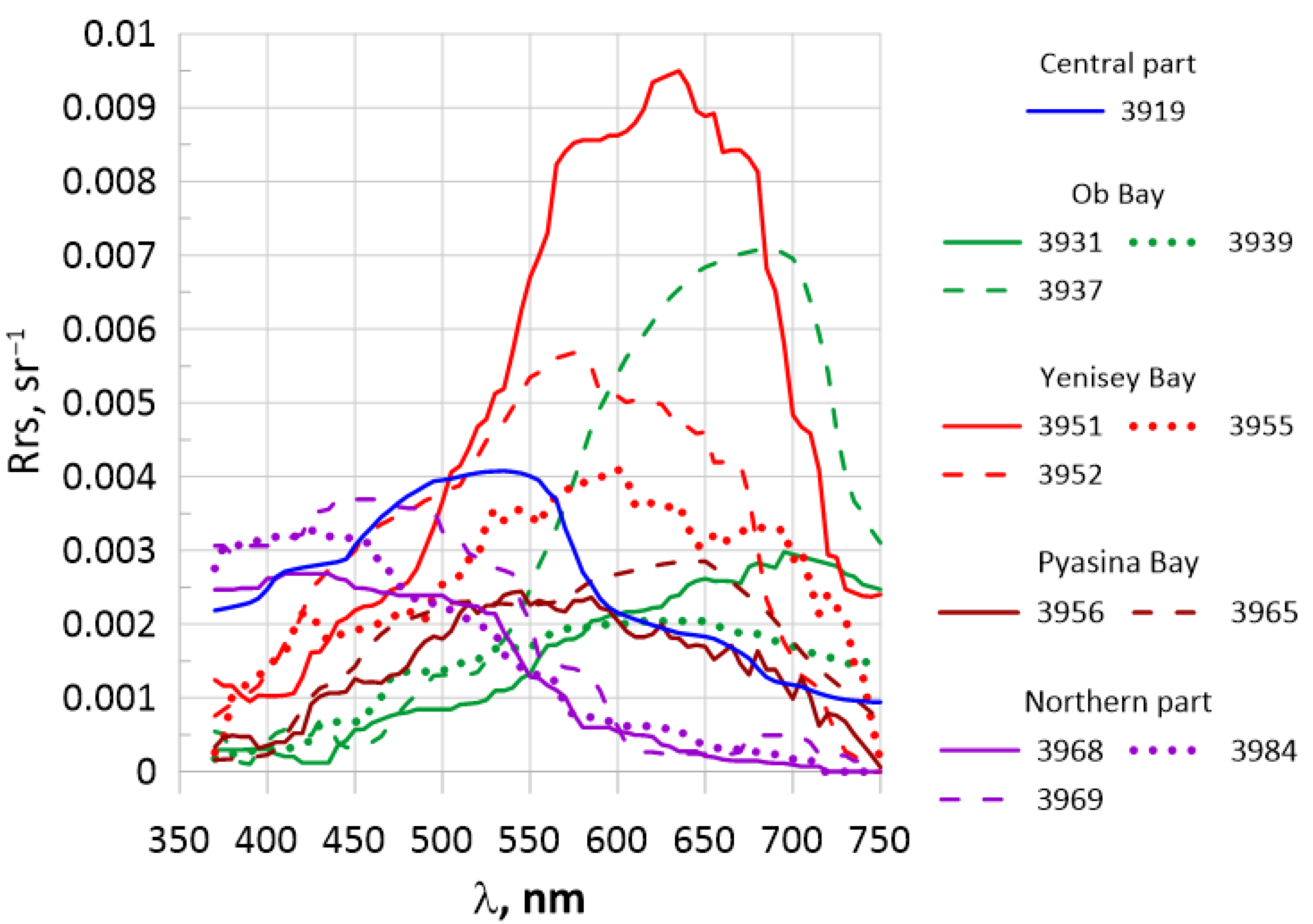
3.1. Field Measurements of Rrs

Figure 4 shows 12 remote sensing reflectance spectra measured in situ, 10 of which correspond to the simultaneous chlorophyll sampling, and 2 spectra (stations 3919 and 3984) correspond to a pixel for which a wide variety of satellite data was obtained. Measurements were affected by weather conditions, resulting in the appearance of some noise; measurement time during which the data were averaged ranged from 5 to 20 min, so the state of smoothness is also different.

There can be seen a distinct difference between measurements in the northern part (stations 3984, 3968 and 3969) and measurements in river plums and estuary zones. The northern part has in fact oceanic conditions, the only source of impurities being the melting of ice. The water is actually “blue”, the maxima of Rrs lay in range 400–450 nm, and the effective wavelengths are 476 and 485 nm for stations 3968 and 3969, respectively. Station 3919 in the central part shows an intermediate type, the Rrs maximum is shifted towards longer wavelengths, and the monotonous decrease towards the short waves shows higher CDOM influence than for northern waters. The rest of the spectra were taken in the estuarine zones and show the strong effect of river runoff, including high CDOM absorption (which is one of the main optically significant components of river waters), causing minima in the short-wave range and high backscattering resulting in increased Rrs (stations 3937, 3951, 3952).

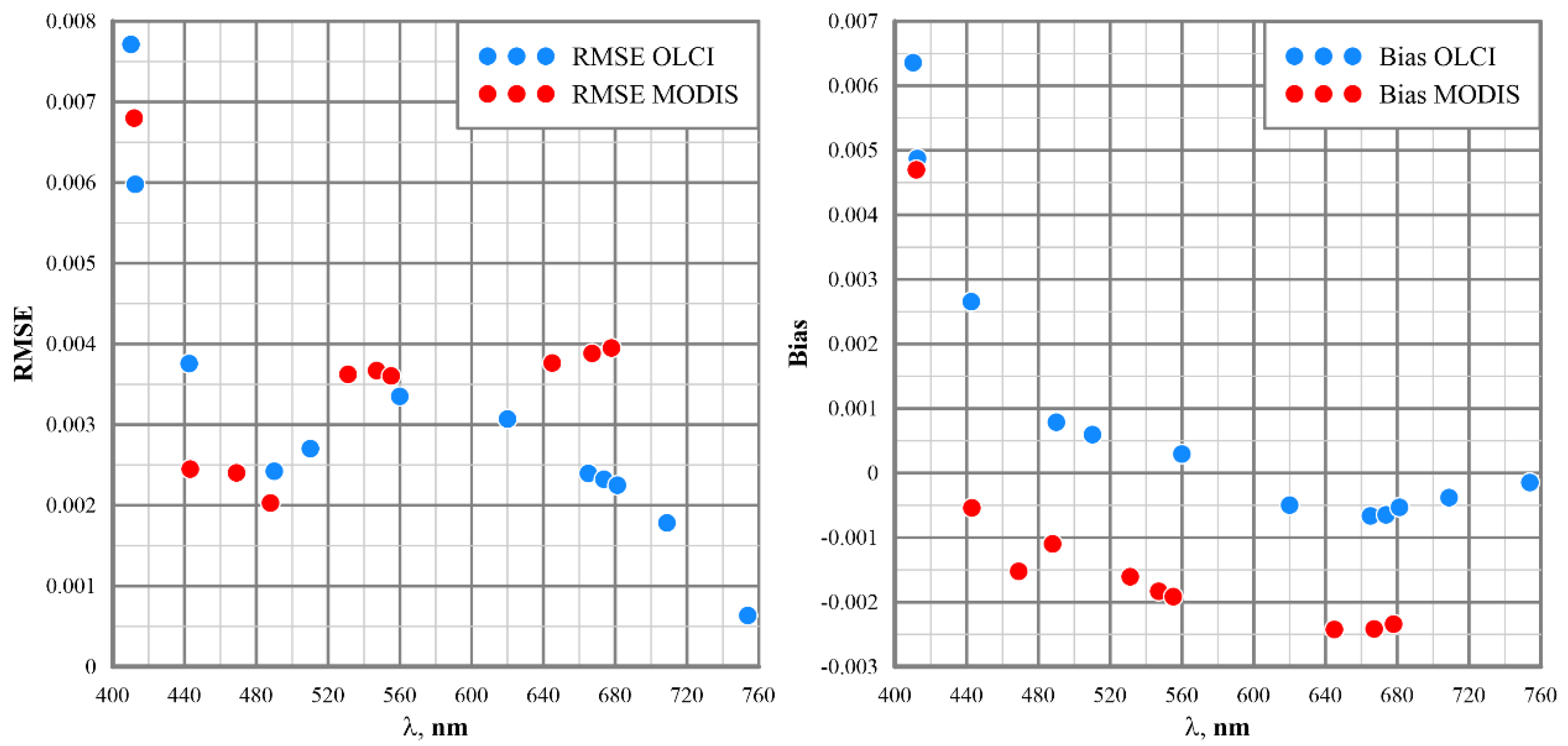
3.2. Comparison of In Situ and Remote Sensing Rrs Spectra

The examples of Rrs spectra obtained as a result of remote and in situ measurements are shown below in Figure 5. Stations are located in different parts of the sea (coastal and open) to show that high discrepancy between satellite and in situ data is not the specific feature of the coastal zone.

Station 3919 is located in the central part of the Kara Sea. The in situ spectrum (Figure 5a) shows the predominance of absorption over backscattering resulting in low Rrs values and the decrease towards short wavelengths. Such spectral shape may indicate the presence of dissolved colored organics and phytoplankton pigments. MODIS and VIIRS Rrs spectra have similar values to the in situ spectra in the range of 450–700 nm. All three MODIS Rrs spectra have a minimum at 443 or 469 nm and a maximum at 412 nm, which is not confirmed by in situ measurements. VIIRS has a significant discrepancy at 443 nm. The OLCI spectrum shows a monotonous decrease with wavelength, not consistent with the shape of in situ reflectance. The range 500–700 nm is where satellite and in situ data are closest to each other.

Station 3937 is located deep in the Ob Bay. The in situ reflectance spectrum is dominated by CDOM, and the maximum is shifted to 680 nm. OLCI Rrs spectra are highly overestimated, one in range 400–550 nm, the other in the whole spectral range. Generally, OLCI Rrs reproduce the spectral shape of the in situ spectra in the range of 500–750 nm. The MODIS spectral range does not include channels >700 nm, so the in situ maximum near 680 nm cannot be reproduced. The minimum near 450–500 nm in satellite spectra is not consistent with the in situ measurements.

Station 3951 is located in the estuary zone of the Yenisei River. A significant influence of river runoff was observed, as evidenced by the nature of the spectrum: the minimum Rrs values in the short-wave range are induced by high absorption by nonliving organics; high absolute values compared to other stations indicate the presence of large amounts of suspended sediments. All three sensors reproduce the shape of the in situ spectra except for the short-wave range. Satellite sensors show minimal Rrs values at 450–500 nm, while in situ spectrum has a minimum near 400 nm.

Station 3984 in the northern part of the Kara Sea is characterized by less organic influence than at stations 3919 and 3951, since the maximum reflectance is observed in the short-wavelength part of the visible spectrum. The spectral shape corresponds to oceanic waters [51]. OLCI data are significantly higher in short-wave range and have negative values in channels >700 nm.

It is important to note that a common feature of all remote sensed data obtained in this study is an overestimation of the Rrs in the short-wave range. Even if the spectral shape corresponds to that of in situ data in the range of 500–700 nm, the short-wave part of the MODIS spectra has the same structure—high values at 412 nm, then a minimum. Moreover, negative values are observed in the long-wave range in OLCI data. These errors could be caused by atmospheric correction algorithms, but a detailed study of this problem is beyond the scope of the current study.

RMSE and bias of MODIS sensor were calculated using 9 Rrs spectra from 9 satellite images and OLCI—using 34 Rrs spectra obtained from 18 images. It was not possible to calculate RMSE and bias for VIIRS due to insufficient data. The RMSE and bias are shown in Figure 6. Regular overestimation of Rrs produces maximal RMSE at 412 nm for MODIS and at 400 nm for OLCI sensors. Bias for MODIS is negative for all channels except 412 nm, showing that in an average satellite, Rrs are lower than in situ. For OLCI, the negative bias occurs in the range >600 nm; for the rest of the channels, satellite Rrs are overestimated.

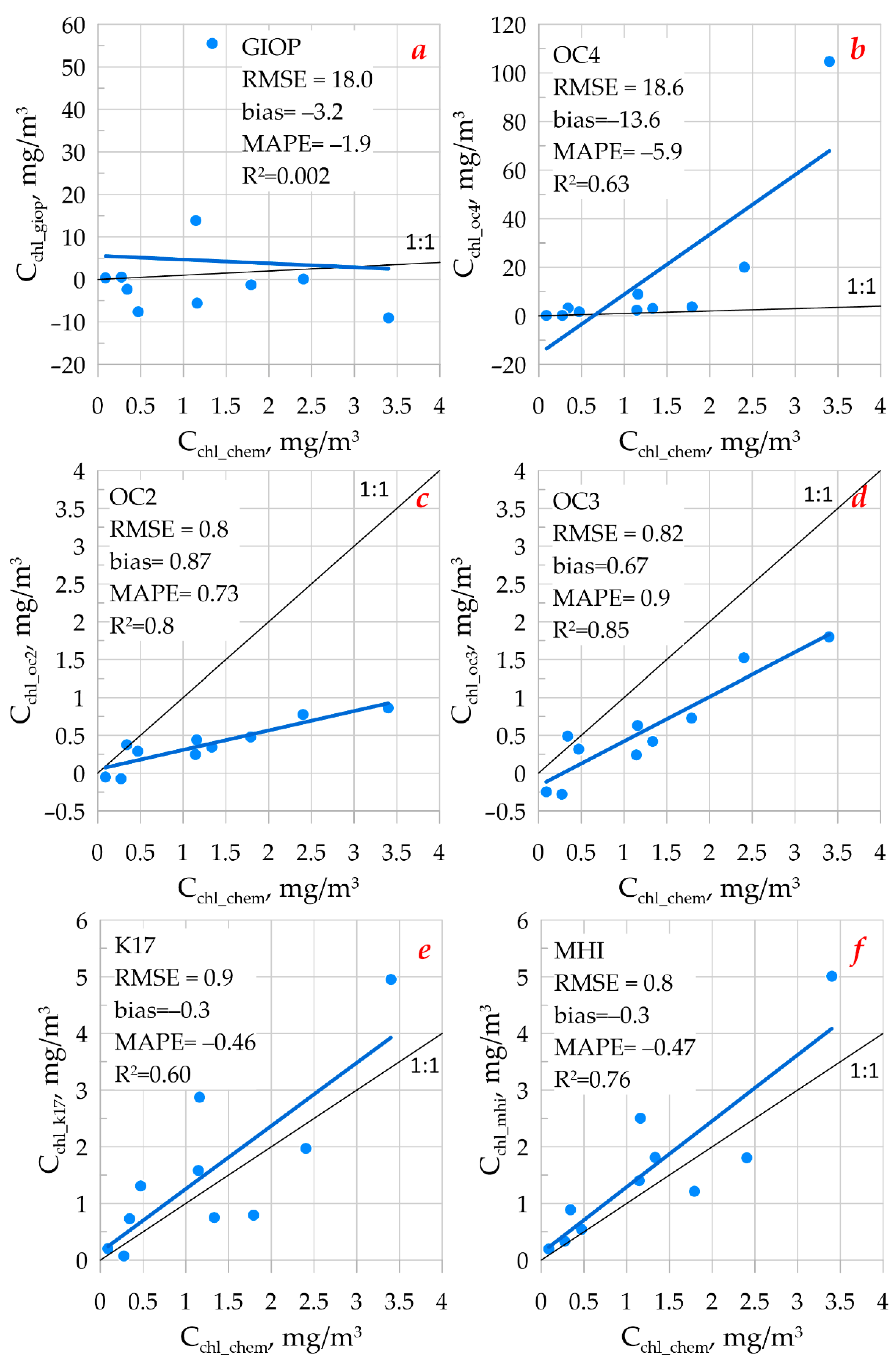
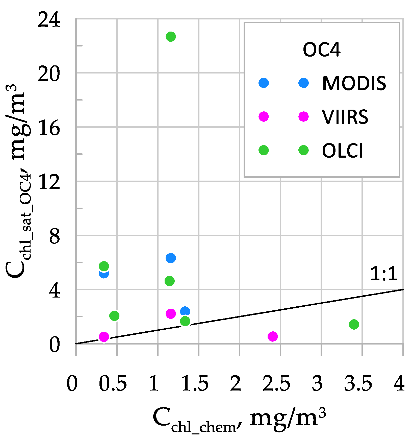
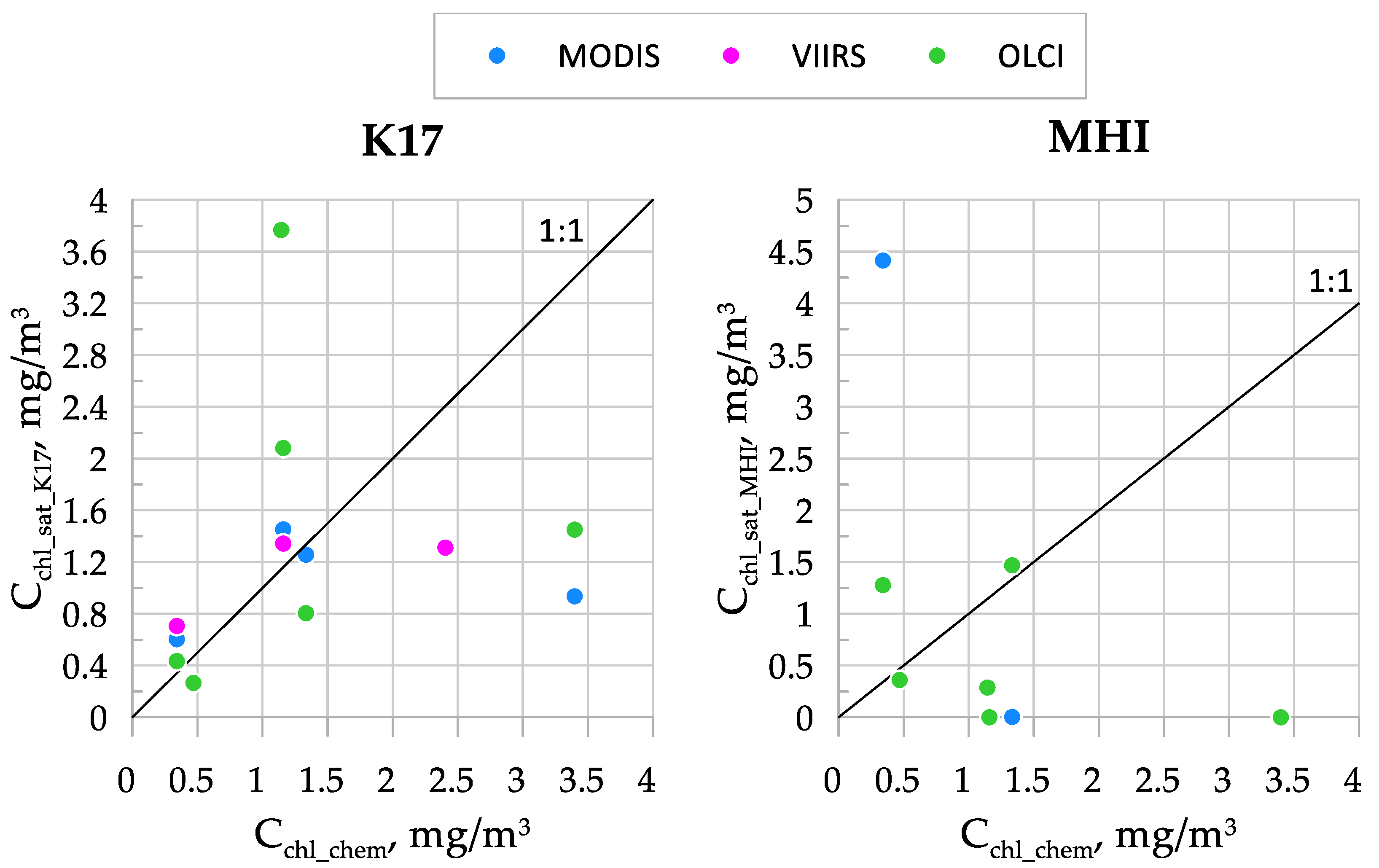
3.3. Comparison of the Different Chlorophyll Algorithms

The correlation between chlorophyll-a concentrations obtained with OCx, K17, and MHI algorithms and in situ chlorophyll range from 0.6 to 0.85. The correlation is significant at 1% level, p-values are 0.001, 0.001, 0.005, 0.006, and 0.001 for OC2, OC3, OC4, K17, and MHI, respectively.

Table 2. Chlorophyll-a concentrations (mg/m³) calculated using in situ Rrs data.

	Station	In Situ	GIOP	OC2	OC3	OC4	K17	MHI
Ob Bay	3931	2.41	0.05	0.78	1.53	19.98	1.97	1.81
	3937	3.40	−9.07	0.86	1.8	104.80	4.96	5.01
	3939	1.79	−1.22	0.48	0.73	3.71	0.79	1.22
Yenisey Bay	3951	1.16	−5.59	0.44	0.63	8.92	2.87	2.50
	3952	1.14	13.85	0.25	0.24	2.39	1.59	1.40
	3955	1.33	55.47	0.34	0.42	3.07	0.75	1.81
Pyasina Bay	3956	0.47	−7.58	0.29	0.32	1.63	1.31	0.54
	3965	0.34	−2.29	0.38	0.49	3.21	0.74	0.89
Northern part	3968	0.27	0.59	−0.07	−0.28	0.14	0.07	0.33
	3969	0.09	0.40	−0.05	−0.25	0.20	0.21	0.20

and Figure 7 present the comparison between these data. The GIOP algorithm gives completely unrealistic results (negative chlorophyll-a concentrations). OC2 and OC3 show the highest correlations, but produce negative chlorophyll-a concentrations in the case of clear water in the northern part of the Kara Sea. A correlation between OC4 results and in situ data is mostly due to the large range of OC4 results. K17 and MHI algorithms show the best performance in terms of all three metrics: MAPE, bias, and RMSE. The values of RMSE are 0.9 and 0.8, respectively, compared to 18.0 and 18.6 for GIOP and OC4 algorithms. OC2 and OC3 algorithms show close values of RMSE, 0.8 and 0.82, but the bias and MAPE values are lower for the K17 and MHI algorithms. GIOP, OC4, K17, and MHI algorithms tend to overestimate the chlorophyll-a concentration, but to different degrees. The values of bias are all negative, but for the K17 and MHI algorithms bias equals −0.3, when for the GIOP and OC4 it is −3.2 and −13.6, respectively. The results of K17 and MHI are overestimated by 46% and 47% and OC4 results by 590%. OC2 and OC3 give underestimated results, by 73% and 90%, respectively.

Table 3. Chlorophyll-a concentrations (mg/m³) provided as standard satellite product (OC4) and calculated using regional algorithms (K17 and MHI) from satellite Rrs data.

	Station	In Situ	OC4			K17			MHI
			MODIS	VIIRS	OLCI	MODIS	VIIRS	OLCI	MODIS	OLCI
Ob Bay	3931	2.41	-	0.53	-	-	1.31	-	-	-
	3937	3.40	-	-	1.43	0.93	-	1.45	-	0.002
	3939	1.79	-	-	-	-	-	-	-	-
Yenisey Bay	3951	1.16	6.32	2.21	22.67	1.45	1.34	2.08	0.002	0.001
	3952	1.14	-	-	4.63	-	-	3.77	-	0.29
	3955	1.33	2.38	-	1.67	1.26	-	0.80	0.003	1.47
Pyasina Bay	3956	0.47	-	-	2.06	-	-	0.27	-	0.36
	3965	0.34	5.20	0.50	5.72	0.60	0.71	0.43	4.41	1.28

shows a few available satellite OC4 chlorophyll-a concentrations for MODIS, VIIRS, and OLCI sensors, as well as the results of the application of regional K17 and MHI algorithms to satellite Rrs. It should be noted that the time difference between satellite observations and in situ sampling reached 24 h, which may affect the accordance between satellite and in situ data. Visual comparison of these data is shown in Figure 8 and Figure 9.

Figure 8 shows the relation between satellite OC4 and in situ chlorophyll-a concentrations. It was difficult to obtain a sufficient dataset because of cloudiness conditions in the Arctic, so only 12 pairs of in situ remote sensed data are presented. The correlation between satellite and in situ data is insignificant (R² = 0.008). The values of Cchl are, on average, overestimated by 500%.

The results of K17 in Figure 9 are overestimated, on average, by 23% and the results of MHI algorithm by 100%. Correlation is insignificant in both cases (for K17 R² = 0.03 and for MHI is 0.008). The advantage of the K17 is that it successfully processes every Rrs spectrum, while the MHI algorithm gives near-zero chlorophyll in some cases. MHI algorithm was not applicable to VIIRS data because of the small number of spectral channels.

4. Discussion

The obtained in situ reflectance spectra represent different hydro-optical conditions, from blue oceanic water to brown river runoff. At the same time, the discrepancies between remote sensed and in situ reflectance change with wavelength in a similar way, as shown in Figure 6; although a certain part of this discrepancy can be attributed to a natural temporal variability of seawater properties, since the time difference is relatively large. In the Kara Sea, the terrigenous CDOM, supplied by Ob and Yenisei rivers, represents the main CDOM source. In the Arctic Ocean, the contribution of CDOM absorption at 443 nm to the total non-water absorption can reach ~50%. It was shown that systematic differences in chlorophyll retrievals resulting from different ocean color models are related to each model’s ability to account for the absorption of light by CDOM [18]. Accordingly, the variability of CDOM absorption in the surface layer is associated with the speed of river runoff propagation and can vary significantly depending on weather conditions [48]. Variability of CDOM content in seawater can lead to the Rrs changes in short-wave channels, which can be one of the reasons of discrepancy between in situ and satellite measurements.

RMSE in Figure 6 has a strong maximum in short-wave channels as a result of a regular overestimation of Rrs for both MODIS and OLCI scanners (Figure 6, left panel). Examples of such overestimation can be seen in Figure 5. The RMSE minimum near 480 nm corresponds to the wavelength where remote sensed data becomes underestimated. Bias (Figure 6, right panel) shows positive values in short-wave channels and negative in the long-wave ones, which again reflects how the shape of the reflectance spectra is distorted during satellite measurements. This inaccuracy can lead, for example, to incorrect calculations of chlorophyll-a concentration using the OC4 algorithm, which is based on the selected maximum Rrs value in the short-wave range.

During the research, it was shown that GIOP results do not correlate with in situ data, and OC4 algorithm significantly overestimates in situ C_chl, especially for high concentrations. Both algorithms give results with high RMSE, 18.0 and 18.6, respectively, and negative bias.

The OC4 algorithm, in the case of chlorophyll-a concentrations >0.2mg/m³, uses two Rrs channels: one with maximal values in short-wave range and another near 550 nm. The obvious problem is with Cchl > 2 mg/m³ (Figure 7b) where OC4 results are highly overestimated. A possible explanation may be that, in the OC4 algorithm, low Rrs values in short-wave channels are correlated with high chlorophyll content, not taking into account terrigenous CDOM brought by river runoff. It is interesting how the OC4 results are 10 and more times higher than in situ Cchl for stations 3931 and 3937 in the Ob Bay, and 2–5 times higher than in situ for stations 3951, 3952, and 3955 in the Yenisey Bay, showing the difference in the river water composition and indicating the strong influence of CDOM on the accuracy of the algorithms, as it was shown by other researchers [52].

The chlorophyll-a concentrations of the MODIS, VIIRS, and OLCI color scanners shown in Table 2 and in Figure 8 were also obtained using OC4 algorithm. The overestimation and general lack of correlation can be attributed to the time difference between in situ and remote sensing observations. Another reason can be the errors in atmospheric correction due to Arctic conditions, leading to increased Rrs in short-wave channels.

In the GIOP model, the parameter of nonliving organics absorption spectral slope is constant and equals $S_{dg}=0.018$ nm⁻¹, and phytoplankton absorption $a_{ph}^{*}\left(\lambda \right)$ is taken according to the Bricaud model [44]. The basic chlorophyll concentration for the Bricaud absorption model is estimated using OC4 method, which was shown to overestimate it. It is known that these input parameters work poorly in the case of water bodies affected by river runoff [53]. For the Kara Sea, the influence of river runoff is significant, as it contributes a third part of the total river runoff in the Arctic Ocean [54]. Since the contributions of $Chla$ and $a_{cdom}\left(\lambda \right)$ are calculated from $a_{ph}^{*}\left(\lambda \right)$, without taking into account the actual distribution of optically active components in the water column, the errors can occur. It was shown in [55] that the GIOP model can be tuned for rather turbid waters with user-defined $S_{dg}$, $S_{bp}$, and $a_{ph}^{*}\left(\lambda \right)$, which significantly improves accuracy and eliminates existing errors. However, such optimization requires additional complex measurements of the absorption and scattering properties of the studied waters [5,56].

Regional K17 and semi-analytical MHI algorithms also give overestimated results, which is especially noticeable for C_chl > 1 mg/m³ (Figure 7c,d). The RMSE for both algorithms is significantly smaller compared to the standard GIOP and OC4 models; bias is negative as well. Compared to OC2 and OC3 algorithms, the MAPE and bias metrics are smaller for K17 and MHI. The main fault of OC2 and OC3 algorithms in this study appeared to be negative results and overall underestimation of the chlorophyll concentration. In general, the performance of the K17 and MHI algorithms is acceptable; R² values are 0.60 and 0.76. K17 was reported by its authors to have an R² = 0.43, but in this study, we obtained the value 0.6. This is probably due to the fact that the original dataset for the development of K17 was collected during a few years and different seasons, and the current study only took one month, which led to a higher correlation. As for K17, it was shown by its authors [14] that in estuarine zones, where chlorophyll-a is not the main factor affecting Rrs spectra, it can provide inconsistent results. Since the algorithm is based on two spectral channels, 531 and 547 nm, there is the possibility that it does not take into account all variations of the Rrs spectral shape in the 550–700 nm range, which can be a more pronounced indicator of the chlorophyll content. Even though the spectral channels chosen for the K17 algorithm are not under the strong influence of CDOM, in estuarine zones there still exists the possibility that variations in CDOM absorption affect the results. The application of K17 to satellite Rrs data showed similar chlorophyll concentrations, where in situ chlorophyll differed two or three times; it also gave double the overestimated concentrations for the same in situ point. This is the effect of the distorted Rrs spectral shape rather than of the poor performance of the algorithm, since the application of the K17 algorithm to the in situ Rrs data have shown much more reliable results.

The overestimation of the chlorophyll-a concentration by the MHI semi-analytical algorithm, in the case of in situ reflectance, can be compensated for by the proper selection of CDOM spectral slope S, which requires CDOM spectral absorption measurements in water samples. The results indicate that S = 0.015 nm⁻¹ is too low for oceanic waters, and the right values can reach 0.025 nm⁻¹ [52]. The MHI algorithm can vary the S parameter decreasing it in case of river runoff down to 0.008 nm⁻¹, which also corresponds to known data [48]. So, the CDOM spectral slope appears to be the main source of errors in this algorithm. Previously, it was estimated for the Black Sea, that the variation of S in the range of 0.015–0.02 nm⁻¹, leads to a 25% error in calculated chlorophyll-a concentration [35]. In the case of satellite Rrs, the MHI algorithm cannot estimate the real effective wavelength, which strongly depends on the spectral shape. The increase in the Rrs in short-wave range leads to the shift of the effective wavelength towards shorter waves and consequently, to the incorrect choice of the optimization procedure. As a result, near-zero chlorophyll-a concentrations are obtained, while the algorithm is trying to compensate the lack of absorption with increased CDOM concentrations. The performance of the K17 and MHI algorithms shows the need for the proper atmospheric correction for the Arctic region.

The overestimation of chlorophyll-a concentration is not unique to the Kara Sea. As shown in [57] for the East China Sea and in [58] for the La Plata region, a significant improvement in satellite algorithms is required for estuarine areas. This overestimation is attributed not only to the strong CDOM absorption [59], but also to the unsatisfactory atmospheric correction, which leads to errors in the channels responsible for CDOM absorption [10]. It is possible to carry out validation of CDOM absorption and additional validation of chlorophyll concentration using fluorimetric methods [59,60]. The small amount of available in situ data might also be responsible for the insufficient accuracy of the algorithms. The presence of a flow-through and spectral fluorimeter will be a good opportunity to obtain high quality in situ measurements for further work. Comprehensive algorithm validation based on field measurements is essential for developing regional algorithms in complex water areas.

5. Conclusions

During the 58th cruise of R/V “Akademik Ioffe” to the Kara Sea in August 2021, new data on the concentration of chlorophyll-a and the sea reflectance were obtained, which were compared with satellite data of the MODIS, VIIRS, and OLCI sensors. As a result of the comparison, it was shown that overestimated values of the remote sensing reflectance are observed in short-wave channels, which can be a consequence of errors in the operation of atmospheric correction algorithms. Chlorophyll-a concentrations calculated using the standard and regional algorithms based on satellite data of the remote sensing reflectance were also considered. It was shown that standard satellite products, as well as regional algorithms applied to remote sensing data in the Kara Sea, cannot provide valid chlorophyll-a concentrations, and the modification of atmospheric correction algorithms is required.

Global models GIOP and OCx, as well as regional algorithms K17 and MHI, were applied to in situ reflectance data. The dataset was rather small and probably does not represent all the varieties of optically different waters. Based on a limited amount of data, it was shown that OCx is not suited for such complex water conditions, and GIOP needs a serious tuning according to regional bio-optical features. The regional Black Sea algorithm MHI was adapted to be used for the Kara Sea, and it was shown that with slight tuning it can be applied to both oligotrophic and eutrophic waters. The results of the regional algorithms K17 and MHI show good correlation (0.6 and 0.76, respectively) with in situ chlorophyll-a concentrations, and even if an overestimation is observed, the RMSE and MAPE of these two algorithms are relatively low. Chlorophyll-a concentrations <1 mg/m³ obtained by these algorithms can be considered reliable, and for the higher concentrations, the 50% overestimation should be taken into account. In the future, having obtained new in situ data, we plan to continue this study of the algorithms’ performance. The development of regional algorithms, as well as their improvement, is an important future activity in order to increase the accuracy in determination of the inherent bio-optical characteristics of seawater.

References

1. Demidov, A.B.; Sheberstov, S.V.; Gagarin, V.I. Estimation of the annual Kara Sea primary production. Oceanology 2018, 58, 369–380. [Google Scholar] [CrossRef]
2. Park, J.-Y.; Kug, J.-S.; Bader, J.; Rolph, R.; Kwon, M. Amplified Arctic warming by phytoplankton under greenhouse warming. Proc. Natl. Acad. Sci. USA 2015, 112, 5921–5926. [Google Scholar] [CrossRef] [PubMed] [Green Version]
3. Jin, Z.; Charlock, T.P.; Rutledge, K. Analysis of Broadband Solar Radiation and Albedo over the Ocean Surface at COVE. J. Atmos. Ocean. Technol. 2002, 19, 1585–1601. [Google Scholar] [CrossRef]
4. Zhao, D.; Xu, Y.; Zhang, X.; Huang, C. Global chlorophyll distribution induced by mesoscale eddies. Remote Sens. Environ. 2021, 254, 112245. [Google Scholar] [CrossRef]
5. Werdell, P.J.; Franz, B.A.; Bailey, S.W.; Feldman, G.C.; Boss, E.; Brando, V.E.; Mangin, A. Generalized ocean color inversion model for retrieving marine inherent optical properties. Appl. Opt. 2013, 52, 2019–2037. [Google Scholar] [CrossRef] [Green Version]
6. Hu, C.; Lee, Z.; Franz, B. Chlorophyll a algorithms for oligotrophic oceans: A novel approach based on three-band reflectance difference. J. Geophys. Res. 2012, 117. [Google Scholar] [CrossRef] [Green Version]
7. Zavialov, P.O.; Izhitskiy, A.S.; Osadchiev, A.A.; Pelevin, V.V.; Grabovskiy, A.B. The structure of thermohaline and bio-optical fields in the surface layer of the Kara Sea in September 2011. Oceanology 2015, 55, 461–471. [Google Scholar] [CrossRef]
8. Demidov, A.B.; Gagarin, V.I.; Vorobieva, O.V.; Makkaveev, P.N.; Artemiev, V.A.; Khrapko, A.N.; Grigoriev, A.V.; Sheberstov, S.V. Spatial and vertical variability of primary production in the Kara Sea in July and August 2016: The influence of the river plume and subsurface chlorophyll maxima. Polar Biol. 2018, 41, 563–578. [Google Scholar] [CrossRef]
9. Qu, B.; Gabric, A.J.; Matrai, P.A. The satellite-derived distribution of chlorophyll-a and its relation to ice cover, radiation and sea surface temperature in the Barents Sea. Polar Biol. 2006, 29, 196–210. [Google Scholar] [CrossRef]
10. Glukhovets, D.; Kopelevich, O.; Yushmanova, A.; Vazyulya, S.; Sheberstov, S.; Karalli, P.; Sahling, I. Evaluation of the CDOM Absorption Coefficient in the Arctic Seas Based on Sentinel-3 OLCI Data. Remote Sens. 2020, 12, 3210. [Google Scholar] [CrossRef]
11. Lewis, K.M.; Mitchell, B.G.; Van Dijken, G.L.; Arrigo, K.R. Regional chlorophyll a algorithms in the Arctic Ocean and their effect on satellite-derived primary production estimates. Deep Sea Res. Part II Top. Stud. Oceanogr. 2016, 130, 14–27. [Google Scholar] [CrossRef]
12. Kopelevich, O.V.; Sahling, I.V.; Vazyulya, S.V.; Glukhovets, D.I.; Sheberstov, S.V.; Burenkov, V.I.; Karalli, P.G.; Yushmanova, A.V. Bio-Optical Characteristics of the Seas, Surrounding the Western Part of Russia, from Data of the Satellite Ocean Color Scanners of 1998–2017; OOO “VASh FORMAT,”: Moscow, Russia, 2018; ISBN 9785907092471. (In Russian) [Google Scholar]
13. Antonov, N.P.; Kuznetsov, V.V.; Kuznetsova, E.N.; Tatarnikov, V.A.; Belorustseva, S.A.; Mitenkova, L.V. Ecology of Arctic cod Boreogadus saida (Gadiformes, Gadidae) and its fishery potential in Kara Sea. J. Ichthyol. 2017, 57, 721–729. [Google Scholar] [CrossRef]
14. Demidov, A.B.; Kopelevich, O.V.; Mosharov, S.A.; Sheberstov, S.V.; Vazyulya, S.V. Modelling Kara Sea phytoplankton primary production: Development and skill assessment of regional algorithms. J. Sea Res. 2017, 125, 1–17. [Google Scholar] [CrossRef]
15. Morel, A.; Prieur, L. Analysis of variations in ocean color. Limnol. Oceanogr. 1977, 22, 709–722. [Google Scholar] [CrossRef]
16. Glukhovets, D.I.; Goldin, Y.A. Surface desalinated layer distribution in the Kara Sea determined by shipboard and satellite data. Oceanologia 2020, 62, 364–373. [Google Scholar] [CrossRef]
17. Osadchiev, A.A.; Frey, D.I.; Shchuka, S.A.; Tilinina, N.D.; Morozov, E.G.; Zavialov, P.O. Structure of the Freshened Surface Layer in the Kara Sea During Ice-Free Periods. J. Geophys. Res. Oceans 2021, 126, e2020JC016486. [Google Scholar] [CrossRef]
18. Drozdova, A.N.; Nedospasov, A.A.; Lobus, N.V.; Patsaeva, S.V.; Shchuka, S.A. CDOM Optical Properties and DOC Content in the Largest Mixing Zones of the Siberian Shelf Seas. Remote Sens. 2021, 13, 1145. [Google Scholar] [CrossRef]
19. Kuznetsova, O.A.; Kopelevich, O.V.; Sheberstov, S.V. Analysis of the chlorophyll concentration in the Kara Sea according to MODIS-AQUA satellite scanner. Issled. Zemli iz Kosm. (Earth Res. Space) 2013, 5, 21–31. (In Russian) [Google Scholar] [CrossRef]
20. O’Reilly, J.E.; Maritorena, S.; Mitchell, B.G.; Siegel, D.A.; Carder, K.L.; Garver, S.A.; Kahru, M.; McClain, C.R. Ocean color chlorophyll algorithms for SeaWiFS. J. Geophys. Res. 1998, 103, 24937–24953. [Google Scholar] [CrossRef] [Green Version]
21. Gordon, H.R.; Wang, M. Retrieval of water-leaving radiance and aerosol optical thickness over the oceans with SeaWiFS: A preliminary algorithm. Appl. Opt. 1994, 33, 443–452. [Google Scholar] [CrossRef]
22. Belanger, S.; Ehn, J.K.; Babin, M. Impact of sea ice on the retrieval of water-leaving reflectance, chlorophyll a concentration and inherent optical properties from satellite ocean color data. Remote Sens. Environ. 2007, 111, 51–68. [Google Scholar] [CrossRef]
23. Wang, M.H.; Shi, W. Detection of Ice and Mixed Ice-Water Pixels for MODIS Ocean Color Data Processing. IEEE Trans. Geosci. Remote Sens. 2009, 47, 2510–2518. [Google Scholar] [CrossRef]
24. Zege, E.; Malinka, A.; Katsev, I.; Prikhach, A.; Heygster, G.; Istomina, L.; Birnbaum, G.; Schwarz, P. Algorithm to retrieve the melt pond fraction and the spectral albedo of Arctic summer ice from satellite optical data. Remote Sens. Environ. 2015, 163, 153–164. [Google Scholar] [CrossRef] [Green Version]
25. Frouin, R.; Deschamps, P.-Y.; Ramon, D.; Steinmetz, F. Improved ocean-color remote sensing in the Arctic using the POLYMER algorithm. In Proceedings of the Remote Sensing of the Marine Environment II, Kyoto, Japan, 29 October–1 November 2012; p. 85250I. [Google Scholar] [CrossRef]
26. König, M.; Hieronymi, M.; Oppelt, N. Application of Sentinel-2 MSI in Arctic Research: Evaluating the Performance of Atmospheric Correction Approaches Over Arctic Sea Ice. Front. Earth Sci. 2019, 7, 22. [Google Scholar] [CrossRef] [Green Version]
27. Kopelevich, O.V.; Sheberstov, S.V.; Vazyulya, S.V.; Zolotov, I.G.; Bailey, S.W. New approach to atmospheric correction of satellite ocean color data. In Proceedings of the Current Research on Remote Sensing, Laser Probing, and Imagery in Natural Waters, Moscow, Russia, 1–3 January 2007; p. 661502. [Google Scholar] [CrossRef]
28. Korchemkina, E.N.; Kalinskaya, D.V. Algorithm of Additional Correction of Level 2 Remote Sensing Reflectance Data Using Modelling of the Optical Properties of the Black Sea Waters. Remote Sens. 2022, 14, 831. [Google Scholar] [CrossRef]
29. Mobley, C.D. Estimation of the remote sensing reflectance from above–water methods. Appl. Opt. 1999, 38, 7442–7455. [Google Scholar] [CrossRef]
30. Molkov, A.A.; Fedorov, S.V.; Pelevin, V.V.; Korchemkina, E.N. Regional Models for High-Resolution Retrieval of Chlorophyll a and TSM Concentrations in the Gorky Reservoir by Sentinel-2 Imagery. Remote Sens. 2019, 11, 1215. [Google Scholar] [CrossRef] [Green Version]
31. Coloured Optical Glass. Specifications. Available online: https://docs.cntd.ru/document/1200023782 (accessed on 28 September 2022).
32. Mueller, J.L.; Fargion, G.S.; McClain, C.R. Ocean Optics Protocols for Satellite Ocean Color Sensor Validation, Revision 5, Volume V: Biogeochemical and Bio-Optical Measurements and Data Analysis Protocols; NASA Tech: Washington, DC, USA, 2003. [Google Scholar]
33. Karalli, P.G.; Kopelevich, O.V.; Sahling, I.V.; Sheberstov, S.V.; Pautova, L.V.; Silkin, V.A. Validation of remote sensing estimates of coccolitophore bloom parameters in the Barents Sea from field measurements. Fundam. Apll. Hydrophys. 2018, 11, 55–63. [Google Scholar] [CrossRef]
34. Korchemkina, E.N.; Mankovskaya, E.V. Bio-optical properties of Black Sea waters during coccolithophore bloom in July 2017. In Proceedings of the 25th International Symposium on Atmospheric and Ocean Optics: Atmospheric Physics, Novosibirsk, Russia, 1–5 July 2019; Volume 11208, pp. 1070–1074. [Google Scholar] [CrossRef]
35. Lee, M.E.; Shybanov, E.B.; Korchemkina, E.N.; Martynov, O.V. Retrieval of concentrations of seawater natural components from reflectance spectrum. In Proceedings of the 22nd International Symposium on Atmospheric and Ocean Optics: Atmospheric Physics, Tomsk, Russia, 30 June–3 July 2016; Volume 10035, pp. 629–643. [Google Scholar] [CrossRef]
36. Arar, E.G.; Collins, G.B. Environmental Protection Agency Method 445.0 In Vitro Determination of Chlorophyll a and Pheophytin a in Marine and Freshwater Algae by Fluorescence, Revision 1.2; Environmental Protection Agency, National Exposure Research Laboratory, Office of Research and Development: Cincinnati, OH, USA, 1997; pp. 1–22.
37. Holm-Hansen, O.; Riemann, B. Chlorophyll a determination: Improvements in methodology. Oikos 1978, 30, 438–447. [Google Scholar] [CrossRef]
38. Oceancolor Web. Available online: https://oceancolor.gsfc.nasa.gov/ (accessed on 14 June 2022).
39. Copernicus Online Data Access. Available online: https://coda.eumetsat.int (accessed on 14 June 2022).
40. Bailey, S.W.; Werdell, P.J. A multi-sensor approach for the on-orbit validation of ocean color satellite data products. Remote Sens. Environ. 2006, 102, 12–23. [Google Scholar] [CrossRef]
41. Sheberstov, S.V. System for batch processing of oceanographic satellite data. Sovr. Probl. DZZ Kosm. 2015, 12, 154–161. (In Russian) [Google Scholar]
42. Maritorena, S.; Siegel, D.A.; Peterson, A.R. Optimization of a semianalytical ocean color model for global-scale applications. Appl. Opt. 2002, 41, 2705–2714. [Google Scholar] [CrossRef] [PubMed]
43. Smith, R.C.; Baker, K.S. Optical properties of the clearest natural waters (200–800 nm). Appl. Opt. 1981, 20, 177–184. [Google Scholar] [CrossRef] [PubMed]
44. Bricaud, A.; Babin, M.; Morel, A.; Claustre, H. Variability in the chlorophyll-specific absorption coefficients of natural phytoplankton: Analysis and parameterization. J. Geophys. Res. Oceans 1995, 100, 13321–13332. [Google Scholar] [CrossRef]
45. Bricaud, A.; Morel, A.; Prieur, L. Absorption by dissolved organic matter of the sea (yellow substance) in the UV and visible domains. Limnol. Oceanogr. 1981, 26, 43–53. [Google Scholar] [CrossRef]
46. Wei, J.; Lee, Z.; Ondrusek, M.; Mannino, A.; Tzortziou, M.; Armstrong, R. Spectral slopes of the absorption coefficient of colored dissolved and detrital material inverted from UV-visible remote sensing reflectance. J. Geophys. Res. Oceans 2016, 121, 1953–1969. [Google Scholar] [CrossRef] [Green Version]
47. Nima, C.; Frette, Ø.; Hamre, B.; Stamnes, J.J.; Chen, Y.C.; Sørensen, K.; Norli, M.; Lu, D.; Xing, Q.; Muyimbwa, D.; et al. CDOM Absorption Properties of Natural Water Bodies along Extreme Environmental Gradients. Water 2019, 11, 1988. [Google Scholar] [CrossRef]
48. Pashovkina, A.; Fedorova, I. Coloured dissolved organic matter in aquatic ecosystems of three representative regions of the Arctic according to the data obtained in year 2019. E3S Web Conf. 2020, 163, 04006. [Google Scholar] [CrossRef]
49. Stedmon, C.A.; Amon, R.M.W.; Rinehart, A.J.; Walker, S.A. The supply and characteristics of colored dissolved organic matter (CDOM) in the Arctic Ocean: Pan Arctic trends and differences. Mar. Chem. 2011, 124, 108–118. [Google Scholar] [CrossRef]
50. Korchemkina, E.N.; Molkov, A.A. Regional bio-optical algorithm for Gorky reservoir: First results. Sovr. Probl. DZZ Kosm. 2018, 15, 184–192. [Google Scholar] [CrossRef]
51. Kuznetsova, O.A.; Kopelevich, O.V.; Burenkov, V.I.; Sheberstov, S.V.; Kravchishina, M.D. Development of the regional algorithm for assessment of suspended matter concentration in the Kara Sea from satellite ocean color data. In Proceedings of the VII International Conference «Current problems in Optics of Natural Waters», Saint Petersburg, Russia, 10–14 September 2013; pp. 177–181, ISBN 9785020383678. [Google Scholar]
52. Lavigne, H.; Van der Zande, D.; Ruddick, K.; Cardoso Dos Santos, J.F.; Gohin, F.; Brotas, V.; Kratzer, S. Quality-control tests for OC4, OC5 and NIR-red satellite chlorophyll-a algorithms applied to coastal waters. Remote Sens. Environ. 2021, 255, 112237. [Google Scholar] [CrossRef]
53. Tilstone, G.H.; Lotliker, A.A.; Miller, P.I.; Ashraf, P.M.; Kumar, T.S.; Suresh, T.; Ragavan, B.R.; Menon, H.B. Assessment of MODIS-Aqua chlorophyll-a algorithms in coastal and shelf waters of the eastern Arabian Sea. Cont. Shelf Res. 2013, 65, 14–26. [Google Scholar] [CrossRef]
54. Dobrovol’skii, A.D.; Zalogin, B.S. Seas of the USSR; Moscow University: Moscow, Russia, 1982. [Google Scholar]
55. Lee, Z.P.; Du, K.; Voss, K.J.; Zibordi, G.; Lubac, B.; Arnone, R.; Weidemann, A. An inherent-optical-property-centered approach to correct the angular effects in water-leaving radiance. Appl. Opt. 2011, 50, 3155–3167. [Google Scholar] [CrossRef] [PubMed]
56. Franz, B.A.; Werdell, P.J. A generalized framework for modeling of inherent optical properties in ocean remote sensing applications. In Proceedings of the Ocean Optics, Anchorage, AK, USA, 27 September–1 October 2010. [Google Scholar]
57. Gong, G.C.; Wen, Y.H.; Wang, B.W.; Liu, G.J. Seasonal variation of chlorophyll a concentration, primary production and environmental conditions in the subtropical East China Sea. Deep. Sea Res. Part II Top. Stud. Oceanogr. 2003, 50, 1219–1236. [Google Scholar] [CrossRef]
58. Garcia, C.A.E.; Garcia, V.M.T. Variability of chlorophyll-a from ocean color images in the La Plata continental shelf región. Cont. Shelf Res. 2008, 28, 1568–1578. [Google Scholar] [CrossRef]
59. Glukhovets, D.I.; Goldin, Y.A. Express method for chlorophyll concentration assessment. J. Photochem. Photobiol. 2021, 8, 100083. [Google Scholar] [CrossRef]
60. Goldin, Y.A.; Glukhovets, D.I.; Gureev, B.A.; Grigoriev, A.V.; Artemiev, V.A. Shipboard flow-through complex for measuring bio-optical and hydrological seawater characteristics. Oceanology 2020, 60, 713–720. [Google Scholar] [CrossRef]
Figure 1. Stations of the 58th cruise of R/V “Academik Ioffe” with the optical measurements. The numbers indicate the stations that will be mentioned later in this article.
Jmse 10 01587 g001
Figure 2. The spectrometer on board R/V “Academik Ioffe”.
Jmse 10 01587 g002
Figure 3. The measurement scheme: (a) the total upwelling radiance, (b) the radiance reflected from the water surface, and (c) the radiance reflected from the white panel.
Jmse 10 01587 g003
Figure 4. Measured spectra of in situ remote sensing reflectance in the 58th cruise of the R/V “Academik Ioffe”.
Jmse 10 01587 g004
Figure 5. In situ and satellite spectra of remote sensing reflectance for the stations in the central part of the Kara Sea (3919, (a)), Ob Bay (3937, (b)), Yenisey Bay (3951, (c)), and the northern part (3984, (d)).
Jmse 10 01587 g005
Figure 6. RMSE and bias of MODIS and OLCI data of remote sensing reflectance.
Jmse 10 01587 g006
Figure 7. Comparison between measured ( C c h l _ c h e m ) and calculated chlorophyll-a concentration: (a)—GIOP; (b)—OC4v.6; (c)—OC2; (d)—OC3; (e)—K17; (f)—MHI algorithms.
Jmse 10 01587 g007
Figure 8. The comparison between measured ( C c h l _ c h e m ) and satellite OC4 chlorophyll-a product from MODIS, VIIRS, and OLCI sensors.
Jmse 10 01587 g008
Figure 9. The comparison between the measured ( C c h l _ c h e m ) chlorophyll-a concentration and results of K17 and MHI algorithms.
Jmse 10 01587 g009