
Effects of Groundwater Inputs to the Hydraulic Circulation, Water Residence Time, and Salinity in a Moroccan Atlantic Lagoon

 ,
,  , , and
Abstract
1. Introduction
2. Materials and Methods
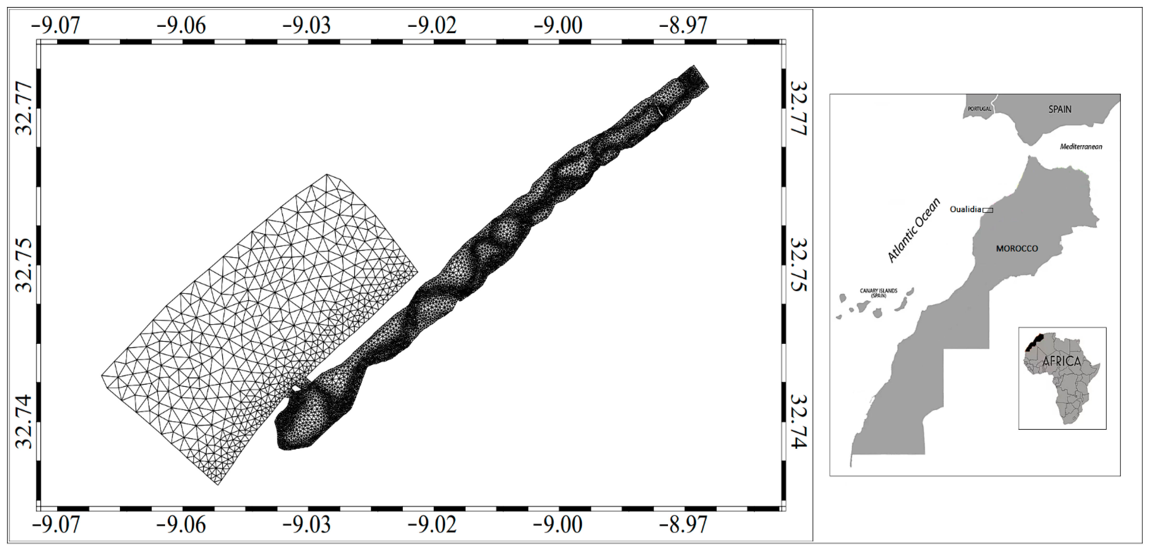
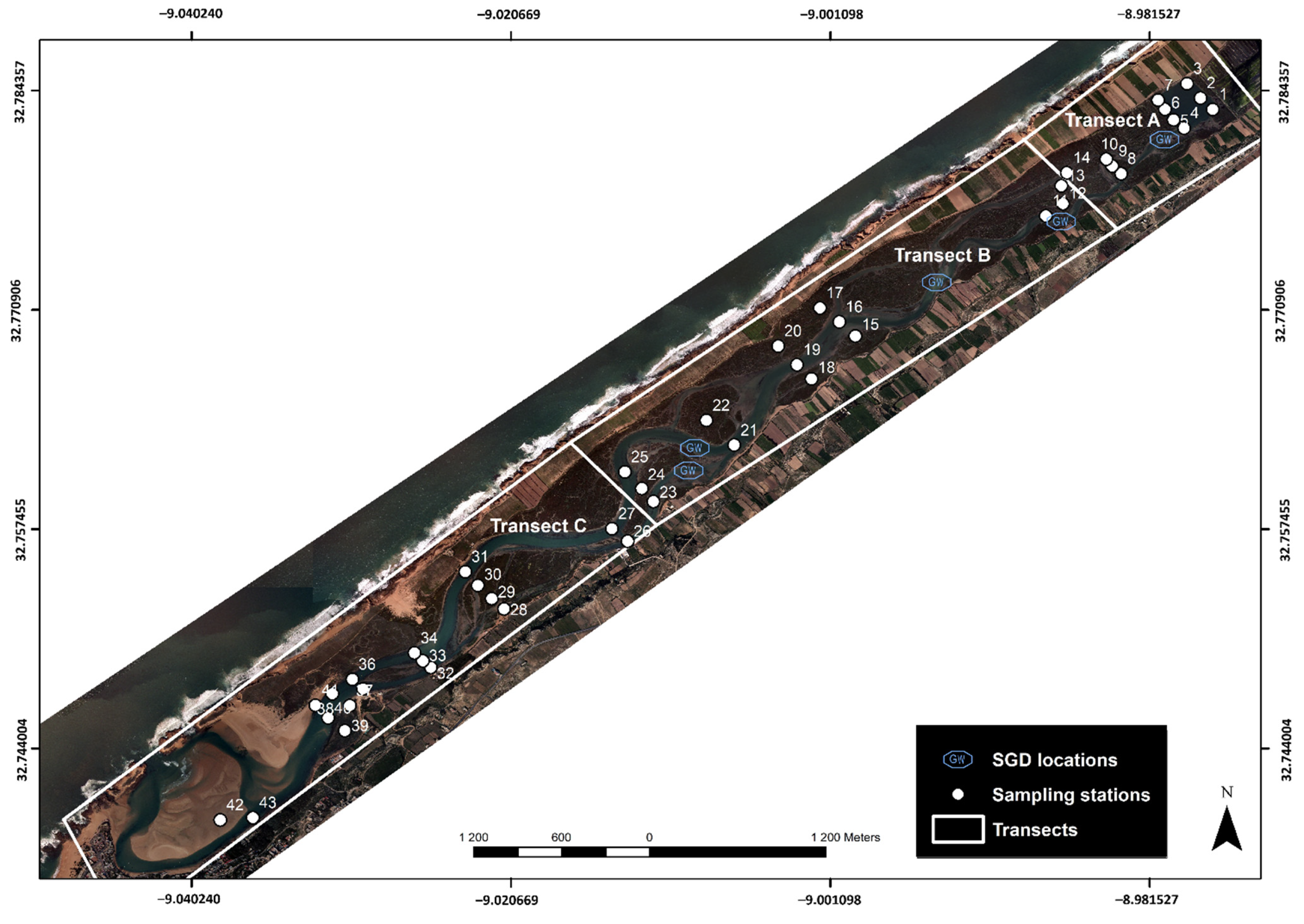
2.1. Study Area
2.2. Data
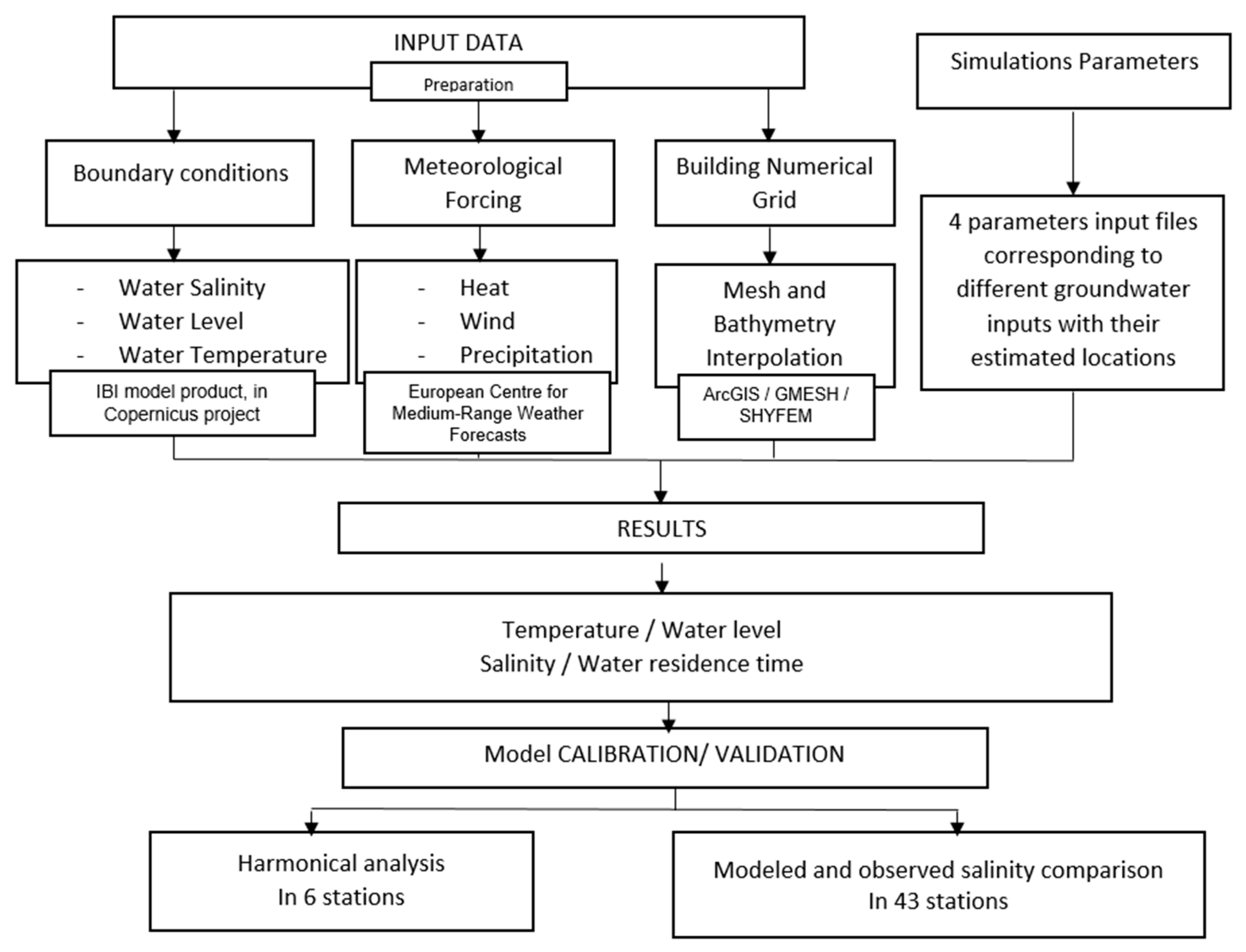
2.3. Model
3. Results
3.1. Calibration and Validation
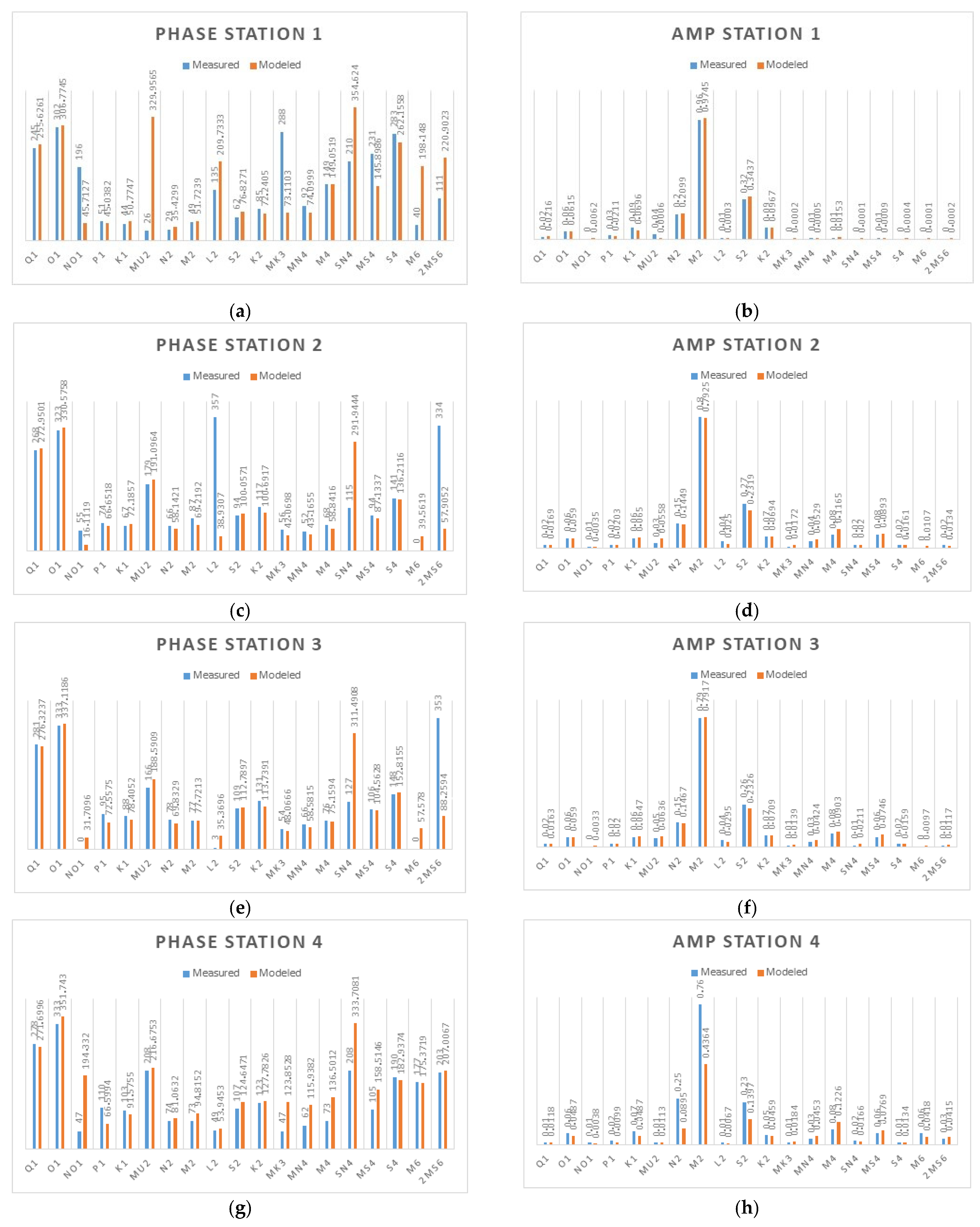
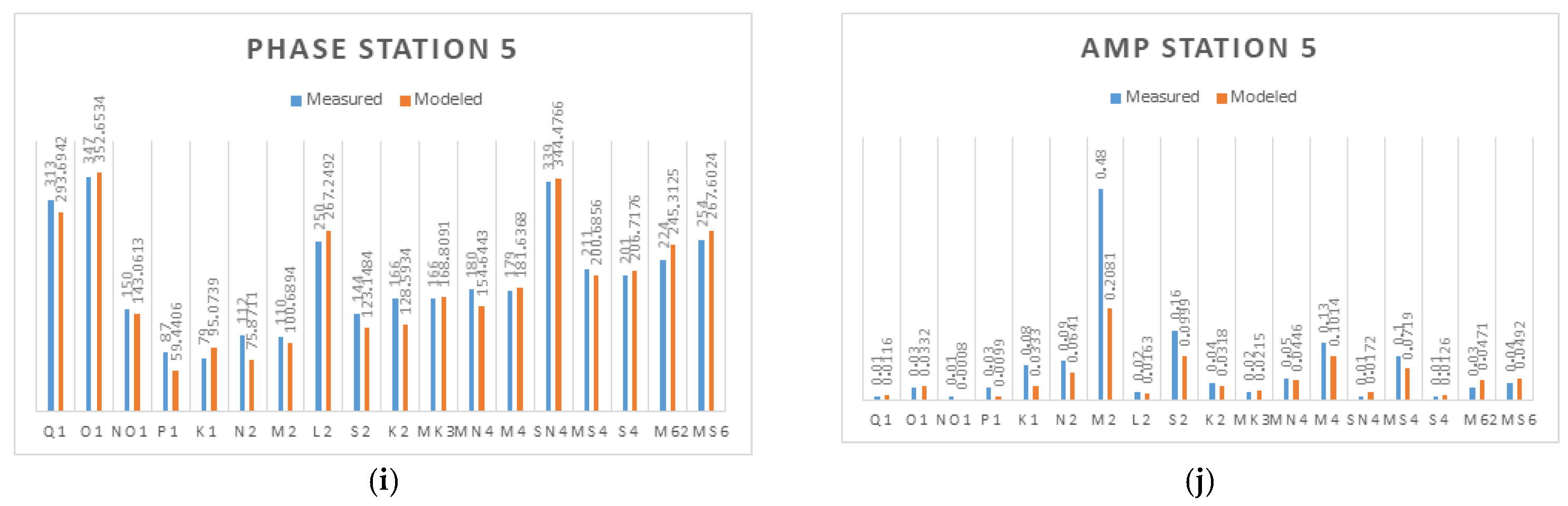
3.1.1. Harmonic Analysis
3.1.2. Validation of SGD Estimation
3.2. Physical Parameters Reproduction
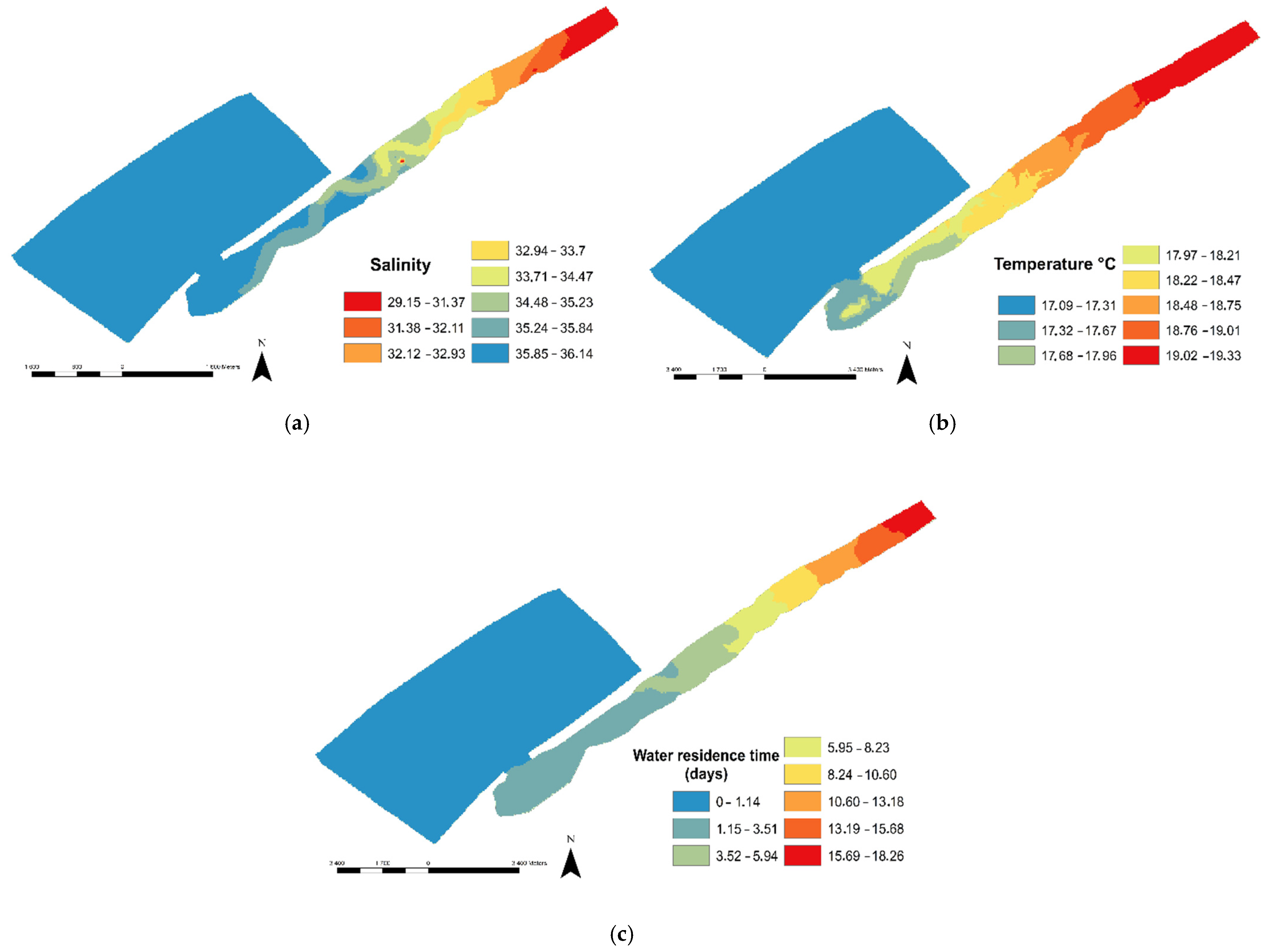
3.2.1. Modeled Salinity
3.2.2. Modeled Water Temperature
3.2.3. Modeled WRT
4. Discussion
4.1. Effect of SGD on Salinity
4.2. Seasonality Effect on Groudwater Input
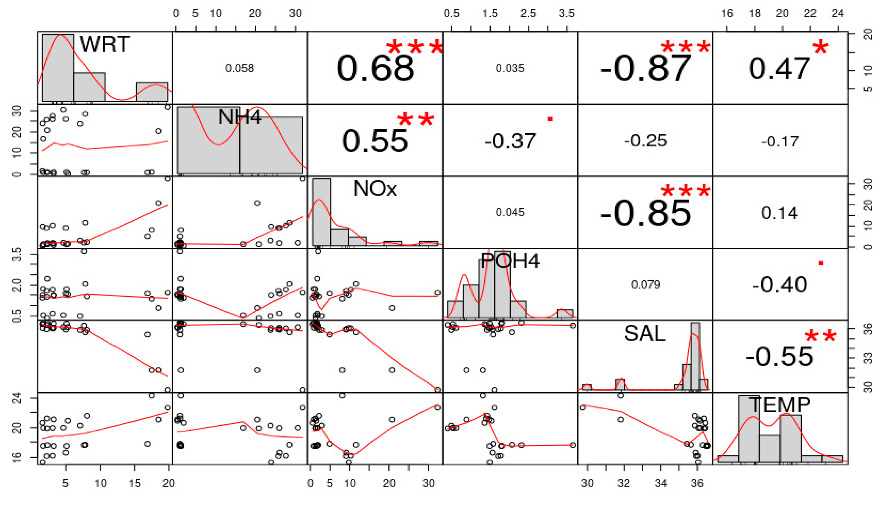
4.3. Nutrients Provided by SGD Discharge and WRT
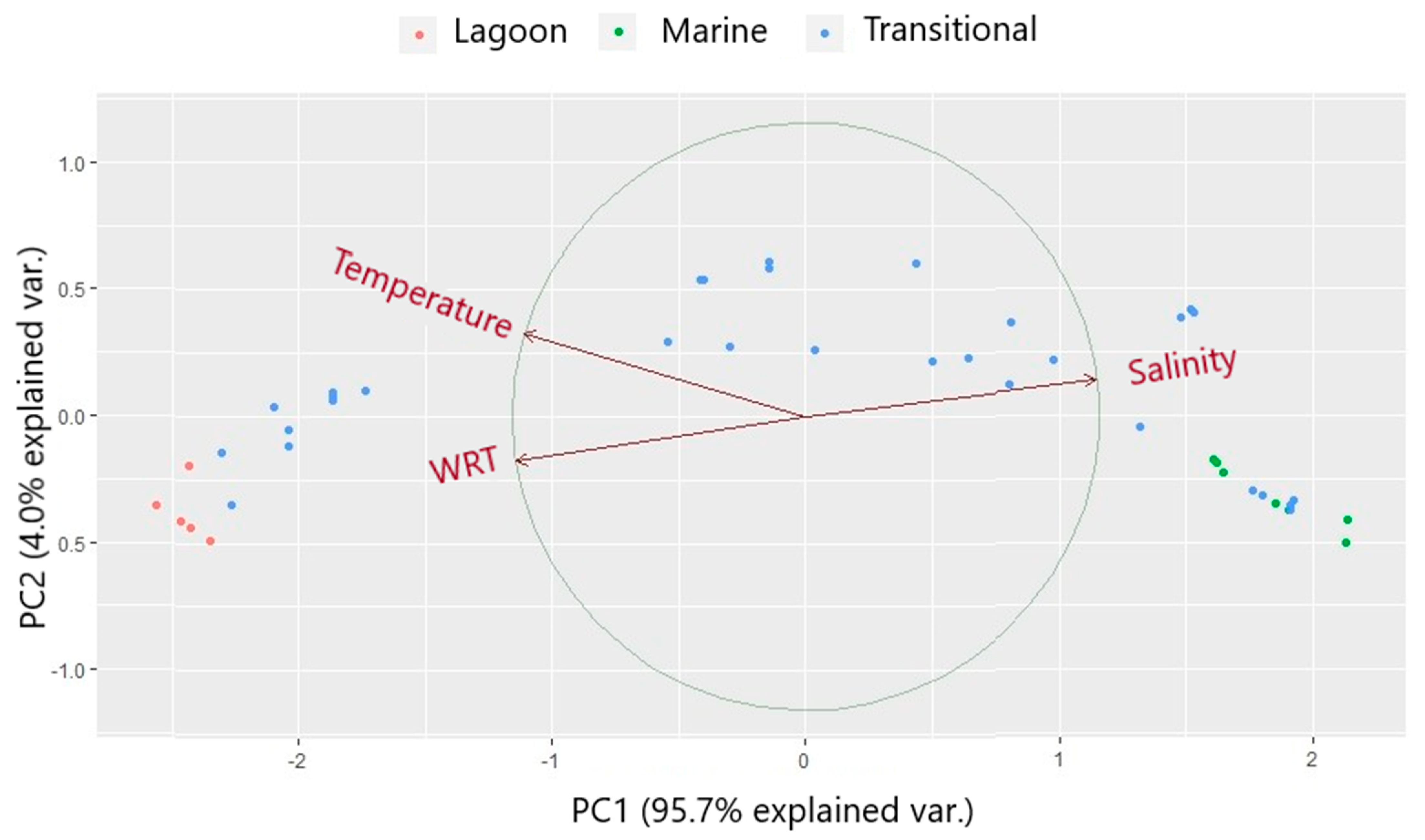
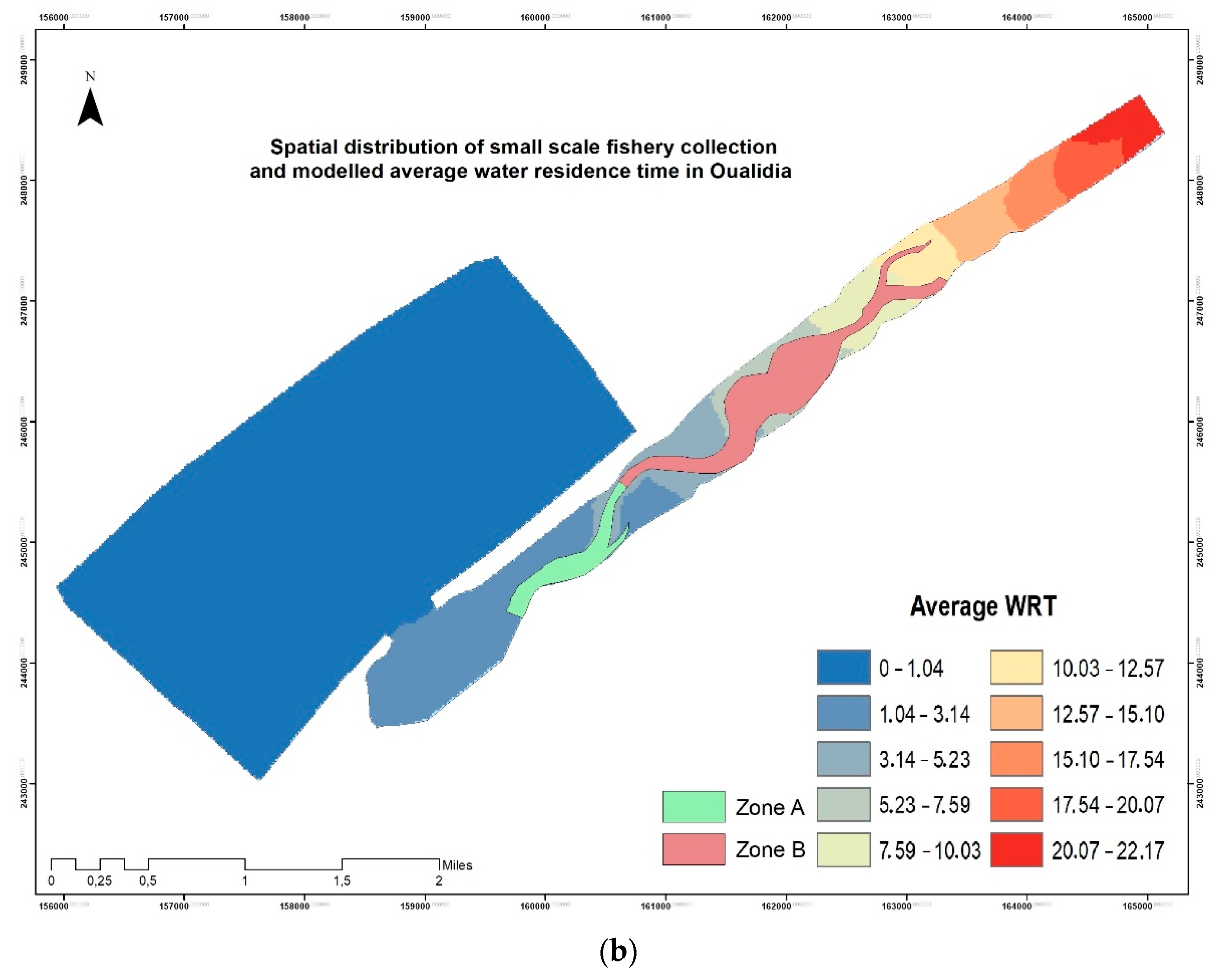
4.4. Physico-Chemical and Biological Gradients in the Lagoon
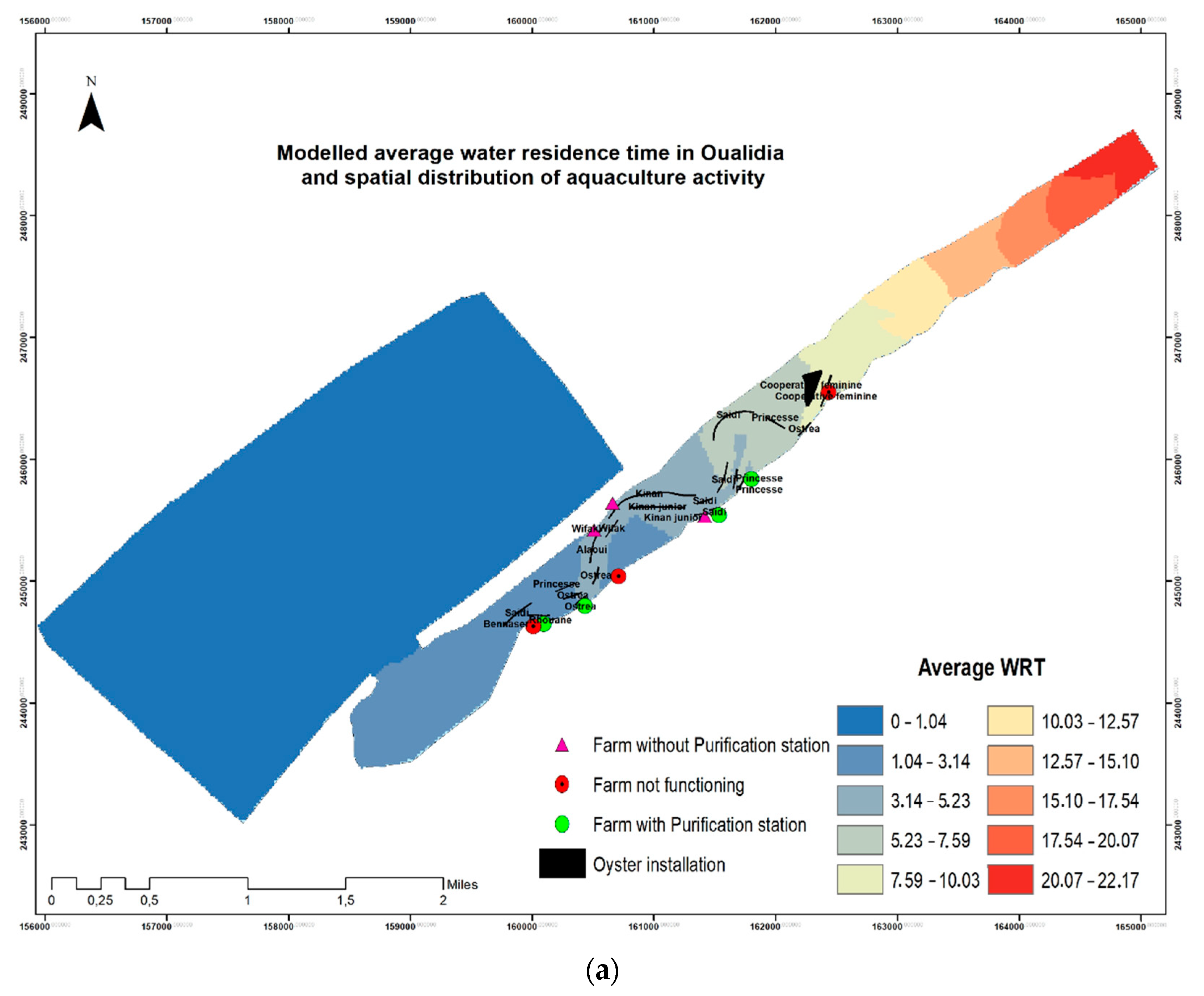
4.5. WRT Relevance to the Oyster Farming in Oualidia
5. Conclusions
Author Contributions
Funding
Institutional Review Board Statement
Informed Consent Statement
Data Availability Statement
Acknowledgments
Conflicts of Interest
Appendix A

| Station 1 | Station 2 | Station 3 | Station 4 | Station 5 | ||||||||||||||||
|---|---|---|---|---|---|---|---|---|---|---|---|---|---|---|---|---|---|---|---|---|
| Phase | Amp | Phase | Amp | Phase | Amp | Phase | Amp | Phase | Amp | |||||||||||
| Measured | Modeled | Measured | Modeled | Measured | Modeled | Measured | Modeled | Measured | Modeled | Measured | Modeled | Measured | Modeled | Measured | Modeled | Measured | Modeled | Measured | Modeled | |
| Q1 | 245 | 255.63 | 0.02 | 0.0216 | 268 | 272.95 | 0.02 | 0.0169 | 281 | 276.32 | 0.02 | 0.0163 | 278 | 271.70 | 0.01 | 0.0118 | 313 | 293.69 | 0.01 | 0.0116 |
| O1 | 302 | 306.77 | 0.06 | 0.0615 | 323 | 330.58 | 0.06 | 0.059 | 333 | 337.12 | 0.06 | 0.059 | 333 | 351.74 | 0.06 | 0.0487 | 347 | 352.65 | 0.03 | 0.0332 |
| NO1 | 196 | 45.71 | 0 | 0.0062 | 55 | 16.11 | 0.01 | 0.0035 | Ns | 31.71 | Ns | 0.0033 | 47 | 194.33 | 0.01 | 0.0038 | 150 | 143.06 | 0.01 | 0.0008 |
| P1 | 51 | 45.04 | 0.03 | 0.0211 | 74 | 66.65 | 0.02 | 0.0203 | 95 | 72.56 | 0.02 | 0.02 | 110 | 66.60 | 0.02 | 0.0099 | 87 | 59.44 | 0.03 | 0.0099 |
| K1 | 44 | 50.77 | 0.09 | 0.0696 | 67 | 72.19 | 0.06 | 0.065 | 88 | 78.41 | 0.06 | 0.0647 | 103 | 91.58 | 0.07 | 0.0487 | 79 | 95.07 | 0.08 | 0.0333 |
| MU2 | 26 | 329.96 | 0.04 | 0.0006 | 179 | 191.09 | 0.03 | 0.0558 | 166 | 188.59 | 0.05 | 0.0636 | 208 | 216.68 | 0.01 | 0.0113 | 112 | 75.87 | 0.09 | 0.0641 |
| N2 | 29 | 35.43 | 0.2 | 0.2099 | 66 | 58.14 | 0.15 | 0.1449 | 78 | 69.83 | 0.15 | 0.1467 | 74 | 81.06 | 0.25 | 0.0895 | 110 | 100.69 | 0.48 | 0.2081 |
| M2 | 49 | 51.72 | 0.96 | 0.9745 | 87 | 69.22 | 0.8 | 0.7925 | 77 | 77.72 | 0.79 | 0.7917 | 73 | 94.81 | 0.76 | 0.4364 | 250 | 267.24 | 0.02 | 0.0163 |
| L2 | 135 | 209.73 | 0.01 | 0.0003 | 357 | 38.93 | 0.04 | 0.025 | 3 | 35.37 | 0.04 | 0.0295 | 49 | 53.94 | 0.01 | 0.0067 | 144 | 123.14 | 0.16 | 0.0999 |
| S2 | 62 | 76.83 | 0.32 | 0.3437 | 94 | 100.06 | 0.27 | 0.2319 | 109 | 112.79 | 0.26 | 0.2326 | 107 | 124.65 | 0.23 | 0.1397 | 166 | 128.59 | 0.04 | 0.0318 |
| K2 | 85 | 72.24 | 0.09 | 0.0967 | 117 | 100.69 | 0.07 | 0.0694 | 131 | 113.74 | 0.07 | 0.0709 | 123 | 127.78 | 0.05 | 0.0459 | 166 | 168.81 | 0.02 | 0.0215 |
| MK3 | 288 | 73.11 | 0 | 0.0002 | 56 | 42.07 | 0.01 | 0.0172 | 54 | 48.07 | 0.01 | 0.0139 | 47 | 123.85 | 0.01 | 0.0184 | 180 | 154.64 | 0.05 | 0.0446 |
| MN4 | 92 | 74.10 | 0.01 | 0.0005 | 52 | 43.17 | 0.04 | 0.0529 | 66 | 58.58 | 0.03 | 0.0424 | 62 | 115.93 | 0.03 | 0.0453 | 179 | 181.63 | 0.13 | 0.1014 |
| M4 | 149 | 149.05 | 0.01 | 0.0153 | 68 | 58.84 | 0.08 | 0.1165 | 76 | 75.16 | 0.08 | 0.0903 | 73 | 136.50 | 0.08 | 0.1226 | 339 | 344.47 | 0.01 | 0.0172 |
| SN4 | 210 | 354.62 | 0 | 0.0001 | 115 | 291.94 | 0.02 | 0.02 | 127 | 311.49 | 0.01 | 0.0211 | 208 | 333.70 | 0.02 | 0.0166 | 211 | 200.68 | 0.1 | 0.0719 |
| MS4 | 231 | 145.90 | 0.01 | 0.0009 | 94 | 87.13 | 0.08 | 0.0893 | 106 | 104.56 | 0.06 | 0.0746 | 105 | 158.51 | 0.06 | 0.0769 | 201 | 206.71 | 0.01 | 0.0126 |
| S4 | 283 | 262.16 | 0 | 0.0004 | 141 | 136.21 | 0.02 | 0.0161 | 148 | 152.82 | 0.02 | 0.0159 | 190 | 182.94 | 0.01 | 0.0134 | 224 | 245.31 | 0.03 | 0.0471 |
| M6 | 40 | 198.15 | 0 | 0.0001 | ns | 39.56 | Ns | 0.0107 | Ns | 57.58 | Ns | 0.0097 | 177 | 175.37 | 0.06 | 0.0418 | 254 | 267.60 | 0.04 | 0.0492 |
| 2MS6 | 111 | 220.90 | 0 | 0.0002 | 334 | 57.91 | 0.02 | 0.0134 | 353 | 88.26 | 0.01 | 0.0117 | 203 | 207.01 | 0.03 | 0.0415 | 313 | 293.69 | 0.01 | 0.0116 |
| Transects | Stations | SGD 0 | SGD 0.05 | SGD 0.1 | SGD 0.2 | Observation |
|---|---|---|---|---|---|---|
| Transect A | S1 | 33.52 | 29.59 | 27.27 | 23.69 | 30.17 |
| S2 | 33.51 | 29.57 | 27.25 | 23.68 | 30.36 | |
| S3 | 33.45 | 29.49 | 27.19 | 23.63 | 30.08 | |
| S4 | 33.63 | 29.82 | 27.55 | 24.05 | 32.56 | |
| S5 | 33.62 | 29.84 | 27.59 | 24.10 | 30.33 | |
| S6 | 33.52 | 29.66 | 27.36 | 23.85 | 32.12 | |
| S7 | 33.49 | 29.57 | 27.26 | 23.70 | 34.15 | |
| S8 | 33.70 | 30.07 | 27.82 | 24.24 | 31.61 | |
| S9 | 33.69 | 30.12 | 27.91 | 24.40 | 32.81 | |
| S10 | 33.68 | 30.12 | 27.91 | 24.45 | 30.78 | |
| S11 | 33.91 | 30.54 | 28.41 | 24.98 | 32.81 | |
| S12 | 33.85 | 30.40 | 28.21 | 24.73 | 32.31 | |
| S13 | 33.83 | 30.42 | 28.27 | 24.83 | 32.24 | |
| S14 | 33.81 | 30.43 | 28.31 | 24.90 | 32.43 | |
| Transect B | S15 | 34.55 | 32.47 | 31.05 | 28.74 | 31.61 |
| S16 | 34.43 | 32.03 | 30.44 | 27.71 | 31.67 | |
| S17 | 34.60 | 32.70 | 31.40 | 29.06 | 31.86 | |
| S18 | 34.73 | 32.99 | 31.79 | 29.80 | 31.16 | |
| S19 | 34.52 | 32.28 | 30.79 | 28.38 | 31.23 | |
| S20 | 34.75 | 33.13 | 32.01 | 30.08 | 32.81 | |
| S21 | 34.67 | 32.74 | 31.44 | 29.28 | 32.75 | |
| S22 | 35.09 | 34.02 | 33.26 | 31.83 | 35.04 | |
| S23 | 35.25 | 33.35 | 33.68 | 32.48 | 33.01 | |
| S24 | 35.00 | 33.66 | 32.73 | 31.20 | 33.13 | |
| S25 | 34.87 | 33.30 | 32.24 | 30.46 | 32.12 | |
| S26 | 35.30 | 34.49 | 33.91 | 32.70 | 32.88 | |
| S27 | 35.02 | 33.73 | 32.85 | 31.35 | 33.58 | |
| Transect C | S28 | 35.74 | 35.67 | 35.63 | 35.53 | 33.26 |
| S29 | 35.74 | 35.67 | 35.63 | 35.53 | 33.70 | |
| S30 | 35.69 | 35.53 | 35.42 | 35.40 | 34.02 | |
| S31 | 35.29 | 34.47 | 33.91 | 32.92 | 34.28 | |
| S32 | 35.45 | 34.91 | 34.53 | 33.86 | 39.30 | |
| S33 | 35.45 | 34.89 | 34.51 | 33.85 | 39.49 | |
| S34 | 35.45 | 34.90 | 34.52 | 33.81 | 39.43 | |
| S35 | 35.51 | 35.05 | 34.73 | 34.16 | 33.77 | |
| S36 | 35.53 | 35.10 | 34.80 | 34.22 | 33.20 | |
| S37 | 35.59 | 35.27 | 35.04 | 34.40 | 32.75 | |
| S38 | 35.55 | 35.15 | 34.88 | 34.37 | 32.88 | |
| S39 | 35.58 | 35.24 | 35.01 | 34.36 | 39.05 | |
| S40 | 35.57 | 35.22 | 34.97 | 34.53 | 39.36 | |
| S41 | 35.56 | 35.20 | 34.94 | 34.49 | 39.17 | |
| S42 | 35.68 | 35.51 | 35.39 | 35.11 | 39.49 |
References
- Newton, A.; Brito, A.C.; Icely, J.D.; Derolez, V.; Clara, I.; Angus, S.; Schernewski, G.; Inácio, M.; Lillebø, A.I.; Sousa, A.I.; et al. Assessing, quantifying and valuing the ecosystem services of coastal lagoons. J. Nat. Conserv. 2018, 44, 50–65. [Google Scholar] [CrossRef]
- Fakir, Y.; Claude, C.; El Himer, H. Identifying groundwater discharge to an Atlantic coastal lagoon (Oualidia, Central Morocco) by means of salinity and radium mass balances. Environ. Earth Sci. 2019, 78, 626. [Google Scholar] [CrossRef]
- Hilmi, K.; Orbi, A.; Lakhdar, J.I.; Sarf, F. Etude courantologique de la lagune de Oualidia (Maroc) en automne. Bull. L’Inst. Sci. Rabat Sect. Sci. Vie 2005, 26–27, 67–71. [Google Scholar]
- Hilmi, K.; Orbi, A.; Lakhdar, J.I. Hydrodynamisme de la lagune de Oualidia (Maroc) durant l’été et l’automne 2005. Bull. L’Inst. Sci. Rabat Sect. Sci. Terre 2009, 31, 29–34. [Google Scholar]
- Maanan, M.; Ruiz-fernandez, A.C.; Maanan, M.; Fattal, P.; Zourarah, B.; Sahabi, M. A long-term record of land use change impacts on sediments in Oualidia lagoon, Morocco. Int. J. Sediment Res. 2014, 29, 10. [Google Scholar] [CrossRef]
- Hilmi, K.; Koutitonsky, V.G.; Orbi, A.; Lakhdar, J.I.; Chagdali, M. Oualidia lagoon, Morocco: An estuary without a river. Afr. J. Aquat. Sci. 2005, 30, 1–10. [Google Scholar] [CrossRef]
- Rharbi, N.; Ramdani, M.; Berraho, A.; Idrissi, A.L. Caractéristiques hydrologiques et écologiques de la lagune de Oualidia, milieu paralique de la côte atlantique marocaine. Mar. Life 2001, 11, 3–9. [Google Scholar]
- García-Oliva, M.; Pérez-Ruzafa, Á.; Umgiesser, G.; McKiver, W.; Ghezzo, M.; De, P.F.; Concepción, M. Assessing the Hydrodynamic Response of the Mar Menor Lagoon to Dredging Inlets Interventions through Numerical Modelling. Water 2018, 10, 959. [Google Scholar] [CrossRef]
- Umgiesser, G.; Canu, D.M.; Cucco, A.; Solidoro, C. A finite element model for the Venice Lagoon. Development, set up, calibration and validation. J. Mar. Syst. 2004, 51, 123–145. [Google Scholar] [CrossRef]
- Holtermann, P.; Burchard, H.; Jennerjahn, T. Hydrodynamics of the Segara Anakan Lagoon. Reg. Environ. Chang. 2009, 9, 245–258. [Google Scholar] [CrossRef]
- Duque, C.; Jessen, S.; Tirado-Conde, J.; Karan, S.; Engesgaard, P. Application of Stable Isotopes of Water to Study Coupled Submarine Groundwater Discharge and Nutrient Delivery. Water 2019, 11, 1842. [Google Scholar] [CrossRef]
- Rodellas, V.; Garcia-Orellana, J.; Masqué, P.; Feldman, M.; Weinstein, Y. Submarine groundwater discharge as a major source of nutrients to the Mediterranean Sea. Proc. Natl. Acad. Sci. USA 2015, 12, 3926–3930. [Google Scholar] [CrossRef]
- Müller, S.; Jessen, S.; Sonnenborg, T.O.; Meyer, R.; Engesgaard, P. Simulation of density and flow dynamics in a lagoon aquifer environment and implications for nutrient delivery from land to sea. Front. Water 2021, 3, 165. [Google Scholar] [CrossRef]
- Menció, A.; Casamitjana, X.; Mas-Pla, J.; Coll, N.; Compte, J.; Martinoy, M.; Pascual, J.; Quintana, X.D. Groundwater dependence of coastal lagoons: The case of La Pletera salt marshes (NE Catalonia). J. Hydrol. 2017, 552, 793–806. [Google Scholar] [CrossRef]
- Sadat-Noori, M.; Santos, I.R.; Tait, D.R.; McMahon, A.; Kadel, S.; Maher, D.T. Intermittently Closed and Open Lakes and/or Lagoons (ICOLLs) as groundwater-dominated coastal systems: Evidence from seasonal radon observations. J. Hydrol. 2016, 535, 612–624. [Google Scholar] [CrossRef]
- Rapaglia, J.; Ferrarin, C.; Zaggia, L.; Moore, W.S.; Umgiesser, G.; Garcia-Solsona, E.; Garcia-Orellana, J.; Masque, P. Investigation of residence time and groundwater flux in Venice Lagoon: Comparing radium isotope and hydrodynamical models. J. Environ. Radioact. 2010, 101, 571–581. [Google Scholar] [CrossRef] [PubMed]
- Umgiesser, G.; Ferrarin, C.; Cucco, A.; De Pascalis, F.; Bellafiore, D.; Ghezzo, M.; Bajo, M. Comparative hydrodynamics of 10 Mediterranean lagoons by means of numerical modeling. J. Geophys. Res. Ocean. 2014, 119, 2212–2226. [Google Scholar] [CrossRef]
- Ferrarin, C.; Razinkovas-Baziukas, A.; Gulbinskas, S.; Umgiesser, G.; Bliūdžiutė, L. Hydraulic Regime-Based Zonation Scheme of the Curonian Lagoon. Hydrobiologia 2008, 611, 133–146. [Google Scholar] [CrossRef]
- Kolerski, T.; Zima, P.; Szydłowski, M. Mathematical Modeling of Ice Thrusting on the Shore of the Vistula Lagoon (Baltic Sea) and the Proposed Artificial Island. Water 2019, 11, 2297. [Google Scholar] [CrossRef]
- Mejjad, N.; Laissaoui, A.; El-Hammoumi, O.; Benmansour, M.; Benbrahim, S.; Bounouira, H.; Benkdad, A.; Bouthir, F.Z.; Fekri, A.; Bounakhla, M. Sediment geochronology and geochemical behavior of major and rare earth elements in the Oualidia Lagoon in the western Morocco. J. Radioanal. Nucl. Chem. 2016, 309, 1133–1143. [Google Scholar] [CrossRef]
- Bidet, J.C.; Carruesco, C. Étude sédimentologique de la lagune de Oualidia (Maroc). Oceanol. Acta 1982, 8–14, 29–37. [Google Scholar]
- Bennouna, A.; Berland, B.; El Attar, J.; Assobhei, O. Eau colorée à Lingulodinium polyedrum (Stein) Dodge, dans une zone aquacole du littoral du Doukkala (Atlantique marocain) Lingulodinium polyedrum (Stein) Dodge red tide in shellfish areas along Doukkala coast (Moroccan Atlantic). Oceanol. Acta 2002, 25, 159–170. [Google Scholar] [CrossRef]
- Somoue, L.; Demarcq, H.; Makaoui, A.; Hilmi, K.; Ettahiri, O.; Ben Mhamed, A.; Agouzouk, A.; Baibai, T.; Larissi, J.; Charib, S.; et al. Influence of Ocean–Lagoon exchanges on spatio-temporal variations of phytoplankton assemblage in an Atlantic Lagoon ecosystem (Oualidia, Morocco). Reg. Stud. Mar. Sci. 2020, 40, 101512. [Google Scholar] [CrossRef]
- Damsiri, Z.; Natij, L.; Khalil, K.; Loudiki, M.; Rabouille, C.; Ettahiri, O.; Bougadir, B.; Elkalay, K. Spatio-temporal nutrients variability in the Oualidia lagoon (Atlantic Moroccan coast). Int. J. Adv. Res. 2014, 2, 609–618. [Google Scholar]
- Khomalli, Y.; Elyaagoubi, S.; Maanan, M.; Razinkova-Baziukas, A.; Rhinane, H.; Maanan, M. Using Analytic Hierarchy Process to Map and Quantify the Ecosystem Services in Oualidia Lagoon, Morocco. Wetlands 2020, 40, 2123–2137. [Google Scholar] [CrossRef]
- El Asri, F.; Zidane, H.; Maanan, M.; Tamsouri, M.; Errhif, A. Taxonomic diversity and structure of the molluscan fauna in Oualidia lagoon (Moroccan Atlantic coast). Environ. Monit. Assess. 2015, 187, 545. [Google Scholar] [CrossRef]
- Zemlys, P.; Ferrarin, C.; Umgiesser, G.; Gulbinskas, S.; Bellafiore, D. Investigation of saline water intrusions into the Curonian Lagoon (Lithuania) and two-layer flow in the Klaipeda Strait using finite element hydrodynamic model. Ocean Sci. 2013, 9, 573–584. [Google Scholar] [CrossRef]
- Wang, J.D.; Connor, J.J. Chapter 13. In Mathematical Modeling of Near Coastal Circulation; Massachusetts Institute of Technology: Massachusetts, MA, USA, 1975. [Google Scholar]
- Lynch, D.R.; Werner, F.E. Three-dimensional hydrodynamics on finite elements. Part I: Linearized harmonic model. Int. J. Numer. Methods Fluids 1987, 7, 871–909. [Google Scholar] [CrossRef]
- Maicu, F.; Abdellaoui, B.; Bajo, M.; Chair, A.; Hilmi, K.; Umgiesser, G. Modelling the water dynamics of a tidal lagoon: The impact of human intervention in the Nador Lagoon (Morocco). Cont. Shelf Res. 2021, 228, 104535. [Google Scholar] [CrossRef]
- Darwish, M.S.; Moukalled, F. TVD schemes for unstructured grids. Int. J. Heat Mass Trans. 2003, 46, 599–611. [Google Scholar] [CrossRef]
- Smagorinsky, J. General circulation experiments with the primitive equations, I. The basic experiment. Mon. Weather Rev. 1963, 91, 99–164. [Google Scholar] [CrossRef]
- Ferrarin, C.; Umgiesser, G. Hydrodynamic modelling of a coastal lagoon: The Cabras lagoon in Sardinia, Italy. Ecol. Model. 2005, 188, 340–357. [Google Scholar] [CrossRef]
- Cucco, A.; Umgiesser, G. Modeling the Venice Lagoon residence time. Ecol. Model. 2006, 193, 34–51. [Google Scholar] [CrossRef]
- Takeoka, H. Fundamental concepts of exchange and transport time scales in a coastal sea. Shelf Res. 1984, 3, 311–326. [Google Scholar] [CrossRef]
- Burau, J.R.; Simpson, M.R.; Cheng, R.T. Data analysis. In Book Tidal and Residual Currents Measured by an Acoustic Doppler Current Profiler at the West End of Carquinez Strait, San Francisco Bay, California, March to November 1988; Hirsch, R.M., Ed.; US Geological Survey: Sacramento, CA, USA, 1993; Volume 92, No. 4064. [Google Scholar]
- Johannes, R.E.; Hearn, C.J. The Effect of Submarine Groundwater Discharge on Nutrient and Salinity Regimes in a Coastal Lagoon off Perth, Western Australia. Estuar. Coast. Shelf Sci. 1985, 21, 789–800. [Google Scholar] [CrossRef]
- Herrera-Silveira, J.A. Salinity and nutrients in a tropical coastal lagoon with groundwater discharges to the Gulf of Mexico. Hydrobiologia 1996, 321, 165–176. [Google Scholar] [CrossRef]
- Haider, K.; Engesgaard, P.; Sonnenborg, T.O.; Kirkegaard, C. Numerical modeling of salinity distribution and submarine groundwater discharge to a coastal lagoon in Denmark based on airborne electromagnetic data. Hydrogeol. J. 2015, 23, 217–233. [Google Scholar] [CrossRef]
- Kelly, R.P.; Moran, S.B. Seasonal changes in groundwater input to a well-mixed estuary estimated using radium isotopes and implications for coastal nutrient budgets. Limnol. Oceanogr. 2002, 47, 1796–1807. [Google Scholar] [CrossRef]
- El-Gamal, A.A.; Peterson, R.N.; Burnett, W.C. Detecting Freshwater Inputs via Groundwater Discharge to Marina Lagoon, Mediterranean Coast, Egypt. Estuaries Coasts 2012, 35, 1486–1499. [Google Scholar] [CrossRef]
- Slomp, C.P.; Van Cappellen, P. Nutrient inputs to the coastal ocean through submarine groundwater discharge: Controls and potential impact. J. Hydrol. 2004, 295, 64–86. [Google Scholar] [CrossRef]
- Santos, I.R.; Chen, X.; Lecher, A.L.; Sawyer, A.H.; Moosdorf, N.; Rodellas, V.; Tamborski, J.; Cho, H.M.; Dimova, N.; Sugimoto, R.; et al. Submarine groundwater discharge impacts on coastal nutrient biogeochemistry. Nat. Rev. Earth Environ. 2021, 2, 307–323. [Google Scholar] [CrossRef]


| Stations | Position X | Position Y | Depth | Tool/Instrument | Sensor Height |
|---|---|---|---|---|---|
| 1 | 495,466 | 3,622,202 | −5.05 m | Tide gauge | 0.27 m |
| 2 | 496,883 | 3,622,553 | −2.17 m | Current meter | 0.22 m |
| CTD | 0.11 m | ||||
| 3 | 498,873 | 3,624,787 | −2.20 m | Tide gauge | 0.24 m |
| Current meter | 0.14 m | ||||
| CTD | 0.11 m | ||||
| 4 | 500,324 | 3,625,534 | −2.06 m | Current meter | 0.14 m |
| 5 | 501,683 | 3,626,651 | −0.89 m | Tide gauge | 0.24 m |
| CTD | 0.08 m |
| Transects | SGD 0 | SGD 0.05 | SGD 0.1 | SGD 0.2 | Observation |
|---|---|---|---|---|---|
| A | 33.66 | 29.97 | 27.74 | 24.23 | 31.77 |
| B | 34.83 | 33.22 | 32.12 | 30.24 | 32.53 |
| C | 35.56 | 35.20 | 34.95 | 34.44 | 36.21 |
| RMSE | 1.76 | 1.26 | 1.90 | 3.87 | - |
| Variable | PC1 | PC2 |
|---|---|---|
| Salinity | 0.990 | −0.122 |
| WRT | −0.986 | 0.156 |
| Temperature | −0.958 | −0.286 |
| Eigenvalue | 2.869 | 0.121 |
| Variance contribution (%) | 95.64 | 4.04 |
| Cumulative variance contribution rate (%) | 95.6 | 99.7 |
| Oyster Farms | Purifications Station | Minimum WRT | Maximum WRT | Average WRT |
|---|---|---|---|---|
| Bennaser (1) | √ | 2.912901 | 2.92307 | 2.917986 |
| Rhouane (2) | √ | 2.968186 | 2.974259 | 2.971223 |
| Ostrea (3) | √ | 3.107552 | 7.579004 | 4.321887 |
| Alaoui (4) | √ | 3.36252 | 3.613524 | 3.48225 |
| Wifak (5) | × | 3.67748 | 3.778902 | 3.733497 |
| Kinan (6) | × | 3.876138 | 4.746943 | 4.289131 |
| Saidi (7) | √ | 2.72293 | 6.702939 | 4.987685 |
| Princesse (8) | √ | 2.999807 | 7.076069 | 5.203157 |
| Kinan junior (9) | × | 3.788272 | 4.099238 | 3.889388 |
| Cooperative feminine (10) | × | 7.027832 | 8.41517 | 7.760968 |
Publisher’s Note: MDPI stays neutral with regard to jurisdictional claims in published maps and institutional affiliations. |
© 2022 by the authors. Licensee MDPI, Basel, Switzerland. This article is an open access article distributed under the terms and conditions of the Creative Commons Attribution (CC BY) license (https://creativecommons.org/licenses/by/4.0/).
Share and Cite
Elyaagoubi, S.; Umgiesser, G.; Maanan, M.; Maicu, F.; Mėžinė, J.; Hilmi, K.; Razinkovas-Baziukas, A. Effects of Groundwater Inputs to the Hydraulic Circulation, Water Residence Time, and Salinity in a Moroccan Atlantic Lagoon. J. Mar. Sci. Eng. 2022, 10, 69. https://doi.org/10.3390/jmse10010069
Elyaagoubi S, Umgiesser G, Maanan M, Maicu F, Mėžinė J, Hilmi K, Razinkovas-Baziukas A. Effects of Groundwater Inputs to the Hydraulic Circulation, Water Residence Time, and Salinity in a Moroccan Atlantic Lagoon. Journal of Marine Science and Engineering. 2022; 10(1):69. https://doi.org/10.3390/jmse10010069
Chicago/Turabian StyleElyaagoubi, Soukaina, Georg Umgiesser, Mehdi Maanan, Francesco Maicu, Jovita Mėžinė, Karim Hilmi, and Artūras Razinkovas-Baziukas. 2022. "Effects of Groundwater Inputs to the Hydraulic Circulation, Water Residence Time, and Salinity in a Moroccan Atlantic Lagoon" Journal of Marine Science and Engineering 10, no. 1: 69. https://doi.org/10.3390/jmse10010069
APA StyleElyaagoubi, S., Umgiesser, G., Maanan, M., Maicu, F., Mėžinė, J., Hilmi, K., & Razinkovas-Baziukas, A. (2022). Effects of Groundwater Inputs to the Hydraulic Circulation, Water Residence Time, and Salinity in a Moroccan Atlantic Lagoon. Journal of Marine Science and Engineering, 10(1), 69. https://doi.org/10.3390/jmse10010069