Abstract
To address the issue of existing automatic irrigation systems’ excessive reliance on electrical power and communication networks, a one-inlet, four-outlet Hydraulically Actuated Irrigation Control Valve (HAICV) was designed that operates based on water pressure variations. Its hydraulic characteristics and flow field features were investigated through experimental and numerical simulation methods. The results indicated that power–function relationships exist between pressure and flow rate, as well as between flow rate and head loss. The flow coefficient and resistance coefficient were found to range within [77.46, 81.06] and [15.94, 17.46], respectively. Dynamic simulations based on User-Defined Functions (UDF) revealed that during the opening process, the internal pressure of the valve spool remains high, with the primary pressure drop concentrated in the outlet region, and the low-pressure zone shrinks as the opening degree increases. A high-velocity band forms at the outlet, with jet flow and turbulence observed at small to medium openings, while the flow field stabilizes after full opening. The unique spool shape and non-straight flow passage structure of the HAICV result in relatively high energy loss, making it suitable for self-pressure irrigation systems. This study provides a theoretical foundation for evaluating its performance and broader applications.
1. Introduction
Valves, serving as the core control components in irrigation systems, directly influence the operational efficiency of the entire pipeline network through their hydraulic characteristics. They enable the precise management of irrigation water by accurately regulating the flow’s on/off status, direction, and rate. Although current automatic irrigation control valves in agricultural systems have successfully addressed the issues of high labor intensity and low efficiency associated with traditional systems, they typically rely on stable power supply and network communication support. This not only increases infrastructure investment costs but also limits their application in remote areas to some extent. In response to this challenge, the authors’ research and development team has created a novel Hydraulic Actuated Irrigation Control Valve (HAICV). This valve operates without the need for external electrical power or communication infrastructure, relying solely on the modulation of the upstream water pressure within the irrigation system to open, close, and switch flow paths. It proves particularly practical in regions with unstable electricity supply or underdeveloped infrastructure. The HAICV extends the applicability of high-efficiency water-saving irrigation technologies, reduces the energy consumption associated with system construction and operation, and aligns with the requirements of sustainable agricultural development. While existing valve design manuals provide detailed descriptions of the hydraulic characteristics of conventional valves, and academic research on directional control valves [1,2,3] has established a comprehensive system ranging from preliminary design to in-depth exploration, the HAICV’s innovative one-inlet/four-outlet configuration and unique hydraulic actuation mechanism result in differences in its flow characteristics, pressure loss patterns, and dynamic performance compared to those of traditional and directional control valves. Consequently, research specifically targeting the HAICV remains necessary and warrants further in-depth investigation.
Research on the hydraulic characteristics of valves typically focuses on flow and pressure indicators under steady-state conditions—including the flow coefficient and resistance coefficient—as well as dynamic valve opening and closing characteristics. This research often employs Computational Fluid Dynamics (CFD) technology to visualize and analyze internal flow patterns. Yu et al. [4] evaluated the accuracy of five types of turbulence models in diaphragm valves, while Brazhenko et al. [5] established a coupled methodology for the structural design and analysis of solenoid valves. Moujaes et al. [6] and Tabrizi et al. [7] utilized CFD to reveal the variations in flow rate and flow resistance coefficient with opening degree and Reynolds number in ball valves. Separately, Sun et al. [8] found that surface roughness can induce deviations in the flow coefficient of butterfly valves. Wang et al. [9] developed a parametric model for the flow resistance coefficient and pressure loss in ball valves. Conversely, Nguyen et al. [10] analyzed the influence of internal bubble formation on the flow characteristics of butterfly valves. Davis et al. [11] employed an axisymmetric model to elucidate flow separation characteristics within a globe valve, noting that the differences among various turbulence models were not significant. In a developmental effort, Wang et al. [12] created a novel butterfly valve based on the projected weighted area, achieving an ideal linear relationship between the flow coefficient and the opening degree. Furthermore, Dumitrache et al. [13] uncovered the velocity and pressure distribution characteristics inside a three-way valve. In addition, Wang [14] and Wang [15], among others, focused on establishing mathematical models for spool displacement. Himr [16], Zhang [17], and Qian [18], in turn, emphasized the analysis of how operational parameters, such as valve static/dynamic characteristics, opening degree, and pressure ratio, influence the flow field and energy consumption. Conversely, Yang [19] and Mo [20] delved into revealing the intrinsic mechanisms by which key factors, such as valve leakage and spool tilt angle, affect flow field characteristics and the flow coefficient.
As a hydraulic control valve whose opening and closing actions are governed by system pressure changes, the HAICV also encounters common challenges inherent to valves of this type. Tsukiji [21] analyzed the key parameters of spool vibration and their influence mechanisms on pressure pulsations. Stosiak et al. [22] refined the mathematical description of the spool’s vibrational motion in directional control valves, indicating that this vibration leads to periodically varying throttling gaps within the valve, consequently causing pressure and flow pulsations. Erickson [23] and Filo [24] investigated the steady-state flow forces acting on the spool and demonstrated that structural improvements to the spool, while enhancing performance, may simultaneously intensify fluid pulsations. Furthermore, the study by Wang [25] on the structure of a four-way valve also provided valuable insights for the present work.
Opening and closing valves involves unsteady flow, which is far more complex than steady-state conditions. The internal flow field continuously changes with the speed and duration of valve operation. Utilizing dynamic mesh technology, Cui et al. [26] investigated the influence of different opening and closing times on the dynamic flow characteristics of a ball valve throughout its operation cycle. Saha et al. [27] explored the response of the internal spool within a pressure-regulating globe valve to variations in inlet pressure. Qian et al. [28] developed a pilot-operated control globe valve, analyzed the dynamic distribution of its internal flow field, and subsequently summarized the relationship between the inlet static pressure and the spool displacement. Guo et al. [29] established criteria for distinguishing between laminar and turbulent flow based on a spool valve and investigated changes in water flow patterns as the opening degree gradually increased using dynamic mesh technology. Zhang [30], Turesson [31], and Kim [32], among others, employed techniques such as dynamic meshing to accurately capture the transient flow fields within pilot-operated and check valves during their opening and closing cycles. Subsequently, Ivancu [33], Hasan [34], and Li [35], respectively, elucidated the influence of dynamic operational characteristics, such as valve stroking speed and opening time, on valve performance. Building on this, Li et al. [36] employed dynamic simulation to optimize the structural design of a check valve, thereby reducing noise and energy loss.
As a novel irrigation valve, the hydraulic performance and internal flow mechanisms of the HAICV have not been fully elucidated through systematic experimental or numerical simulations. Although preliminary tests have verified its basic functional feasibility, there remains a lack of reliable theoretical support and a systematic performance evaluation framework for its promotion to practical engineering applications. To address this, this study established mathematical relationships among pressure, pressure difference, and flow rate of the HAICV under different operating conditions. The obtained hydraulic parameters can provide critical design references for the valve’s application in future irrigation systems. Furthermore, due to the difficulty in directly observing water flow movement within the valve chamber, this study employed dynamic mesh technology and UDF to numerically simulate and analyze the evolution of the internal transient flow field during the HAICV’s opening and closing processes. This aims to reveal its dynamic working mechanisms and provide theoretical references for subsequent structural optimization of the valve body.
2. Materials and Methods
2.1. HAICV Structure
The HAICV is a novel irrigation control valve that utilizes the pressure of water within the pipeline to drive the valve spool along a predetermined trajectory, enabling both rotational and axial motion. Its intended application is as a field control valve in sprinkler or micro-irrigation systems, enabling water supply control from main pipelines to branch pipelines or from branch pipelines to lateral pipelines within irrigation networks. As a purely mechanical device, the HAICV requires neither manual assistance nor electrical power for operation, which simplifies its use compared to other automated control valves. The physical product of the HAICV is shown in Figure 1. The simplified structural model was developed for it using SolidWorks software [37], as shown in Figure 2.
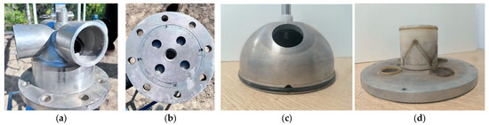
Figure 1.
Physical structure diagram of Hydraulic Actuated Irrigation Control Valve (HAICV): (a) valve housing; (b) valve base; (c) valve spool; (d) guide pillar.
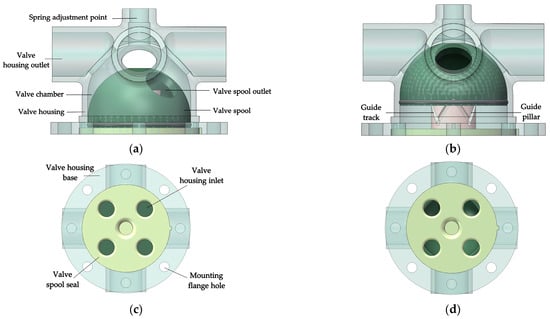
Figure 2.
HAICV simplified structural model: (a) closed state (front view); (b) open state (front view); (c) closed state (bottom view); (d) open state (bottom view).
Both the housing and the spool of the HAICV are cast from aluminum alloy, a material that exhibits excellent corrosion resistance in environments commonly encountered in irrigation systems, such as those involving saline-alkali conditions and chemical fertilizers. It features a DN160 inlet, a DN90 outlet, and primarily consists of components such as the valve housing, the valve spool, guide pillars, and a base plate. In actual irrigation scenarios, the slope of the field terrain affects the actual irrigation effectiveness. The HAICV is equipped with a spring at the top, with one end connected to the top of the valve spool and the other end attached to the top of the valve housing. By adjusting the knob, the spring deformation can be altered, imparting different initial preload forces to the valve spool, thereby adjusting the valve’s opening pressure threshold. As irrigation pipe networks often exhibit a tree-shaped structure, adjusting the spring height alters the opening pressure values of valves at different positions on the main and branch pipes. Under the same water pressure, valves whose spools are subjected to greater preload force from the spring cannot open. Thus, precise irrigation of different plots can be achieved according to the opening sequence defined by irrigation groups. The magnitude of the preload force is characterized by the height of the adjustment knob at the top of the spring (0.6 cm, 0.9 cm, 1.2 cm, 1.5 cm).
As can be seen from the figure, the valve housing adopts a design with a cylindrical lower part and a hemispherical upper part. When the valve spool moves along the guide track to its highest position, i.e., when the HAICV is fully open, the valve spool contacts the hemispherical inner wall of the valve housing. To ensure smooth movement, the HAICV is designed with the inner diameter of the valve housing slightly larger than the outer diameter of the valve spool, creating a reasonable gap. This gap prevents increased movement resistance due to overly small dimensions and effectively avoids significant leakage caused by an excessively large gap. Therefore, from the perspective of structural dimension design, there is no risk of jamming for the valve spool during its entire movement process. However, based on long-term outdoor testing observations, the high-strength nylon material currently used for the guide pillar is prone to thermal expansion under sustained high temperatures and solar exposure, causing dimensional changes in the etched guide tracks on its surface, which subsequently hinders the normal repositioning of the valve spool. To address this issue encountered in practical applications, future improvements can be made by enhancing the material properties of the guide pillar, thereby completely eliminating the risk of valve spool jamming caused by material thermal deformation.
2.2. HAICV Working Principle
To facilitate irrigation in different sectors, each vertical movement of the HAICV’s spool along the guide track is accompanied by a clockwise rotation, ensuring that the water outlet sequentially aligns with sector outlets in a clockwise order. A complete irrigation cycle is described as follows: At the start, the spool outlet is positioned midway between the No. 1 and No. 4 housing outlets, and the HAICV is in the closed state (Figure 3a). At this stage, water accumulates at the four circular inlets at the spool base. When the water pressure at these inlets exceeds the spool’s self-weight, the flow lifts the spool, simultaneously causing it to rotate 45° clockwise along its predetermined track (Figure 3b). Upon reaching the track’s apex, the spool outlet aligns closely with the No.1 housing outlet (Figure 3c), opening the valve and allowing water to discharge through the No.1 outlet into the subsequent pipeline. Upon completion of irrigation, the water supply pressure is discontinued. The self-weight of the HAICV’s spool now exceeds the pressure at the water inlets, causing the spool to descend under gravity. It continues its clockwise rotation by 45° along the predetermined track until it is positioned midway between the No. 1 and No. 2 housing outlets. At this position, the inlet ports on the spool and those on the base become misaligned, thereby closing the water passage and returning the HAICV to the closed state. This constitutes one complete opening and closing cycle of the HAICV. In the subsequent activation, the spool outlet will repeat this process to connect with the No.2 housing outlet. After four such cycles, the HAICV completes its rotation, having irrigated all four sectors in sequence.
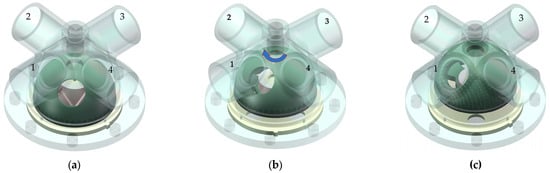
Figure 3.
Schematic diagram of the HAICV opening process: (a) closed state; (b) raised state; (c) open state. The diagram is labeled according to the outlet connection sequence, with arrows indicating the direction of valve spool rotation.
To ensure the HAICV can stably and reliably perform the aforementioned opening/closing and rotation irrigation processes, the pressure settings and pipeline network layout of the irrigation system must meet the corresponding operational conditions for normal actuation. Firstly, the pressure at the system inlet should not fall below the valve’s minimum activation pressure (30 kPa). When the system pressure exceeds this threshold, the HAICV can smoothly complete opening and closing actions. If the pressure is between 20 and 30 kPa, the valve spool will remain in the middle of the guide track in a half-open state, with all four outlets discharging water simultaneously. This results in significant pressure loss, and the outlet pressure approaches atmospheric pressure, failing to meet irrigation requirements. Once the system pressure drops below 20 kPa, the fluid force is insufficient to push the valve spool upward, and the valve remains closed and unable to activate. The same applies when there is no system pressure.
In addition to the inlet pressure requirement, the normal closing of the HAICV also requires that the pressure in the outlet section be lower than that in the inlet section. Therefore, during pipeline network installation, the pipeline elevation must be strictly controlled. In principle, the elevation at the end of the HAICV outlet pipeline should be lower than the valve’s own installation height, or at least not exceed the HAICV installation elevation by more than 0.3 m. If the downstream pipeline is at a higher elevation, after the water supply stops, the retained water in the elevated pipeline will flow back, accumulating in the outlet pipeline and potentially even backflowing into the valve spool area. The backpressure generated by this retained water will hinder the downward movement of the valve spool, preventing the valve from closing properly. If a higher downstream elevation cannot be avoided due to site terrain constraints, a check valve must be installed at an appropriate location to effectively block backflow and ensure unimpeded valve spool operation.
Furthermore, the liquid in the pipeline should maintain a continuous and stable flow state. If the water flow experiences interruption or severe fluctuation, the HAICV may frequently open and close due to pressure variations. This could lead to premature closure and switching of the outlet direction before completing the current irrigation task, disrupting the established irrigation schedule and affecting overall irrigation uniformity and efficiency.
2.3. Experiment on the Hydraulic Characteristics of HAICV
2.3.1. Experimental Setup
Following the completion of the first batch of HAICV products, formal experimentation commenced in June 2024 at an experimental park in Urumqi, Xinjiang Uygur Autonomous Region. Figure 4 shows a schematic diagram of the hydraulic characteristic testing setup, created using Microsoft Office PowerPoint [38]. This system is a closed-loop circulation setup, primarily consisting of a water tank, a variable-frequency centrifugal pump, circulation piping, and the valve under test. During testing, the pump supplies water to the pipeline. The water flow rate in the pipeline is regulated by adjusting the pump speed via a variable frequency drive (VFD). Water from the tank circulates through the system via the pump unit, passing sequentially through an electromagnetic flow meter, an inlet control valve, the valve under test, and an outlet control valve, before returning to the tank to form a closed loop. To ensure the accuracy of flow rate and pressure measurements, the flow meter is installed at a distance of 20D from the test valve. Pressure sensors are mounted at 10D upstream and 10D downstream of the test valve to measure the pressure before and after the valve within the test section, respectively. To prevent the parallel pipelines downstream of the valve from altering the pressure conditions, four separate individual circuits were employed and tested sequentially.
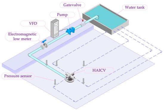
Figure 4.
HAICV hydraulic characteristics experimental setup diagram. The dashed line represents the HAICV return water pipe.
Prior to data acquisition, all system valves were opened and the variable-frequency pump was activated to ensure the entire pipeline was fully primed. The flow rate within the pipeline was adjusted by setting different frequencies on the VFD. For each test point, the system was observed for at least 10 s. A steady state was considered achieved if the variation in each measured quantity did not exceed 1.2% (calculated as the ratio of the difference between the maximum and minimum readings to the average value). The corresponding pressure and flow rate readings were recorded only when a steady state was attained and the flow exhibited no fluctuations. Data was acquired at a sampling frequency of 100 Hz, meaning 100 data points were collected per second. Each test group was repeated ten times to eliminate random errors in the results. These data were used to set the inlet pressure boundary condition for the subsequent numerical simulations and to validate the simulation accuracy.
2.3.2. Parameters Calculation
The flow capacity of an irrigation valve is generally directly influenced by the valve’s structure [39] and the properties of the fluid. The flow coefficient, Kv, is a key metric for evaluating a valve’s flow capacity. It represents the flow rate of fluid passing through the valve under a unit pressure loss across it. Generally, a higher Kv value indicates better flow performance and a lower pressure loss per unit [40,41]. The formula for calculating the flow coefficient is as follows:
The flow coefficient Kv is calculated using Equation (1), where qv is the volumetric flow rate through the valve body (m3/h); ρ is the mass density of the medium at the test temperature (kg/m3); Δpv is the pressure loss across the valve (MPa); and ρ0 is the mass density of pure water at 15 °C, which is the reference condition for the test (kg/m3).
The flow resistance coefficient ζ of an irrigation valve is a parameter that quantifies the pressure loss across the valve. It reflects the flow resistance or energy loss of the medium passing through the valve [42]. The formula for calculating the resistance coefficient is as follows:
where Δpv denotes the pressure loss across the valve (Pa), and v represents the average flow velocity (m/s).
2.3.3. Uncertainty Analysis Method
Due to the inherent fluctuation characteristics of the HAICV’s flow coefficient and resistance coefficient within a certain range, it is challenging to verify the accuracy of the measurement results using conventional methods. Therefore, this study employs uncertainty analysis [43] to evaluate the measurement results. Depending on the method of data acquisition, the sources of data uncertainty can be categorized into Type A and Type B. Type A uncertainty is calculated statistically through repeated measurements, while Type B uncertainty is based on other sources of information, including the calibration data and acquisition accuracy of the experimental instruments. It is evident that a solitary evaluation method is inadequate in accurately reflecting the precision of measurement outcomes. Consequently, a multifaceted evaluation approach is deemed more suitable. To illustrate this, the flow coefficient is selected as the exemplar. The Type A relative uncertainty, uArel (Kv) is calculated using Equations (3)–(6). In a similar manner, the Type A relative uncertainty for the HAICV’s resistance coefficient, uArel (ζ), can be obtained.
where is the sample variance of the flow coefficient, is the mean value of the flow coefficient, n is the number of repeated test groups, S(Kv) is the standard deviation of the flow coefficient, uA(Kv) is the standard uncertainty of the mean flow coefficient, and uArel(Kv) is the Type A relative standard uncertainty of the flow coefficient.
2.4. Numerical Calculations
Experimental research, as a traditional methodology, serves as the foundation for theoretical analysis and numerical methods. It can establish clear mathematical relationships between variables, yielding results that are authentic and reliable. Furthermore, as a form of prospective study, experiments involve pre-designed research objects and factors, resulting in high demonstrative strength. The HAICV investigated in this study features a fully mechanical structure. During experimental testing, it is impossible to directly observe the internal water flow patterns within the valve chamber, making it difficult to analyze the flow characteristics of the medium inside the valve using traditional analytical methods. Therefore, this study employs computational simulation methods to conduct a numerical investigation of the HAICV. The aim is to elucidate the variations in the internal pressure and velocity fields of the valve spool under constant inlet pressure during normal irrigation operation.
2.4.1. Geometric Models and Mesh Generation
This study utilized SolidWorks to construct the three-dimensional geometric models of the HAICV (Figure 2), which were subsequently imported into the Fluent [44] solver for analysis. To enhance computational efficiency, the following treatments were applied to the models: First, the HAICV was simplified to an ideal valve model with a streamlined outlet section of the valve housing. The cutting edge was defined with a right angle and absolutely sharp edges, while the valve spool and valve seat were assumed to be perfectly matched. Finally, given that the spring atop the valve spool has a negligible influence on the flow field, it was omitted from the model.
Figure 5a shows the central cross-sectional structure of the HAICV, which also serves as the reference plane for subsequent flow field analysis. It can be clearly seen from the figure that the internal structure of the HAICV body is divided into two main regions based on function and motion characteristics: the internal flow passage region defined by the valve spool boundary, and the external cavity region formed by the valve housing boundary. During the opening process of the HAICV, these two regions exhibit distinctly different variation characteristics. Due to its fixed structure, the shape and flow area of the internal flow passage within the valve spool remain constant throughout the opening and closing process, ensuring the stability of water flow through the spool. In contrast, the cavity space defined by the valve housing boundary continuously changes as the valve spool rises. The upward movement of the valve spool continuously compresses the top cavity, while the lower flow space correspondingly expands. This complementary relationship between the upper and lower spaces directly influences the distribution and evolution of the flow field within the valve body and provides important structural insights for understanding the dynamic hydraulic characteristics of the HAICV.
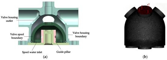
Figure 5.
HAICV flow channel structure and mesh generation: (a) three-dimensional model of the HAICV; (b) mesh of the computational domain.
Due to the irregular geometry of the valve spool, the computational domain was discretized using an unstructured tetrahedral mesh [45]. The final three-dimensional mesh generation of the HAICV is presented in Figure 5b. Prior to conducting numerical analysis, a grid independence study was performed based on the idealized HAICV physical model. With the HAICV fully open, an inlet pressure of 50 kPa was selected as the verification condition. The flow coefficient was calculated using the average pressure and flow rate at the outlet. The differences in the flow coefficient obtained under mesh quantities of approximately 0.30 million, 0.74 million, 1.22 million, and 1.80 million elements are presented in Table 1.

Table 1.
Results of Grid Independence Verification.
It can be observed that when the number of grids exceeds 1.22 million, the increase in the calculated flow coefficient across different grid sizes becomes insignificant. Therefore, considering both computational accuracy and efficiency, a grid size of 1.22 million was selected for the simulation.
2.4.2. Dynamic Mesh and UDF Code Compilation
To simulate the opening motion of the HAICV’s valve spool, dynamic mesh and UDF algorithms were employed to define its movement [46]. Dynamic mesh algorithms primarily include three types: layering, smoothing, and local remeshing. The smoothing method is suitable for tetrahedral meshes in three-dimensional simulations and is more effective for remeshing moving boundaries. However, this process requires iterative computations, which can easily cause excessive deformation of the mesh model, leading to mesh distortion or negative volume elements. To mitigate these issues and ensure both computational convergence efficiency and result accuracy in the numerical simulation, local remeshing was simultaneously applied on the moving boundaries.
The conservation equation for a general scalar φ in an arbitrary control volume V with a moving boundary is expressed as:
where dV represents the moving boundary of the control volume V; ug is the velocity of the moving mesh; Sφ is the source term of the scalar φ; Γ is the dissipation coefficient; ρ is the fluid density; and u is the fluid velocity vector.
UDFs are subroutines written in the C programming language that can be dynamically linked to the Fluent solver. For solving dynamic mesh problems, three commonly used UDFs are: DEFINE_CG_MOTION, used to control the motion of rigid bodies; DEFINE_GEOM, used to control the projection of deforming boundaries; and DEFINE_GRID_MOTION, used to control the motion of individual nodes.
Since the guide track etched on the HAICV guide pillar is arc-shaped with a smooth and rounded surface, and the water flow driving force is sufficient to overcome the motion resistance to ensure the HAICV performs its intended function under normal operating conditions, friction was not considered a primary analytical factor in this study. Based on the design conditions of the mathematical model, the following assumptions are made in this study: the working fluid is an incompressible ideal fluid; gravitational fields are neglected; vertical pressure differences, friction, and other resistances are ignored; there is no leakage between the valve body, valve spool, and valve base, ensuring good sealing performance. During the opening process, the valve spool is subjected to fluid force and gravity; motion initiates when the fluid force exceeds the weight of the valve spool. Considering that the motion of the valve spool combines linear and rotational movements, its dynamics are described by linear motion equations and rotational motion equations.
In the vertical direction, the valve spool is subjected to fluid force and gravitational force. According to Newton’s second law:
where F is the resultant force on the valve spool (N); Ffluid is the constant fluid force applied to the bottom of the valve spool (N); m is the mass of the valve spool (kg).
where θ is the rotation angle of the valve spool, z is the vertical displacement of the valve spool, and h is the displacement along the helical guide track.
The system’s kinetic energy comprises translational kinetic energy and rotational kinetic energy:
where I is the moment of inertia in kg·m2.
Combining Equations (8)–(11) yields:
The above motion equations are compiled into a UDF program and linked with FLUENT to define the motion state of the valve spool. Within a single time step, the moving velocity of the valve spool is iteratively calculated by the UDF. After updating the positions of the surface mesh nodes, the dynamic mesh algorithm adjusts the mesh in the deforming boundary region. Considering factors such as the HAICV’s motion type, the irregular geometry of its surface, and the complexity of boundary mesh changes induced by the movement, a dynamic mesh algorithm combining smoothing and local remeshing was selected. The DEFINE_CG_MOTION function was used to define the motion of the valve spool. Parallel computing functions are introduced via #if !RP_NODE and #if !RP_HOST, followed by the utilization of UDF to control boundary motion. The meanings of the main commands in the opening process UDF are shown in Table 2.
Table 2.
Primary UDF Commands.
2.4.3. Solution Setup
This study employed a transient solver based on the PISO algorithm [47] for the numerical solution of the governing flow equations. The standard k-ε model [48] was selected as the turbulence model due to its wide applicability, good stability, and compatibility with the high-Reynolds-number flow characteristics and curved wall flows inside the HAICV during opening. It can simulate flow details with reasonable accuracy while offering high computational efficiency and strong practical utility in engineering applications. The equations of the standard k-ε model are as follows:
where ρ is the fluid density; μ is the dynamic viscosity of the fluid; Gk is the turbulence kinetic energy generation term due to the mean velocity gradient; σk = 1.0 and σε = 1.3 are the turbulent Prandtl numbers for k and ε, respectively; C1ε = 1.44 and C2ε = 1.92 are the corresponding empirical constants.
In the standard k-ε model, ε is defined by Equation (18):
The turbulent viscosity μt is expressed as a function of the turbulent kinetic energy k and the dissipation rate ε:
where Cμ is an empirical constant with a value of 0.09.
The boundary conditions were set as a pressure inlet of 50 kPa and a pressure outlet with free outflow. In the dynamic mesh settings, both the symmetry plane of the moving domain and its adjacent walls were defined as deforming regions. For pressure-based solvers, the system typically considers an iteration count between 10 and 20 per time step. If convergence is not achieved within this range, the time step size should be appropriately reduced; conversely, it can be increased. Accordingly, the total transient simulation duration in this study was 0.2 s, with a time step size of 2.5 × 10⁻⁴ s. The convergence residual criterion was set to 1 × 10⁻⁵, with a maximum of 20 iterations per time step to ensure adequate convergence of equation residuals. The total calculation involved 800 steps, while all other parameters retained their default software values. Prior to computation, global flow field initialization was performed, and the initial static pressure field in the fluid domain was adjusted to ensure reasonable computational conditions before initiating the solution process.
2.4.4. Simulation Reliability Verification
To validate the accuracy of the numerical calculations, the experimental results were compared with the simulation results, as presented in Table 3.
Table 3.
Simulation Error.
Overall, the error between the simulated and experimental values ranges from 6% to 9%, all falling within the commonly accepted engineering tolerance of ±10% [49]. Furthermore, the error slightly decreases as the inlet pressure increases. The simulated pressure difference is consistently slightly lower than the experimental value [7], exhibiting a systematic negative bias, though the overall fluctuation is small. This discrepancy is likely attributable to the simplification of details such as the valve spool’s chamfer and surface roughness in the 3D model, resulting in a slightly smaller actual flow area and consequently a higher measured pressure difference. Additionally, the complex flow state within the pipeline and the necessity for local mesh remeshing after each displacement step of the valve spool introduce non-orthogonality and sudden volume changes during the remeshing process. This leads to additional numerical dissipation in the momentum equation, causing an underestimation of the pressure difference and thus contributing to the error. Nevertheless, the overall error is controlled within 10%, indicating that the accuracy of the numerical simulation results meets the requirements.
3. Results and Discussion
3.1. Experimental Hydraulic Characteristics of the HAICV
3.1.1. Pressure–Flow Rate Relationship
Valve pressure, flow rate, and pressure loss are two critical parameters essential for the hydraulic calculation and optimal design of irrigation systems. These parameters directly influence core performance indicators, including the hydrodynamic balance of the pipeline network, irrigation uniformity, and system energy consumption. The relationship between the inlet pressure and the flow rate of the HAICV was experimentally measured under free outflow conditions for various spring adjustment heights (0.6 cm, 0.9 cm, 1.2 cm, and 1.5 cm), as presented in Figure 6. A spring height of 0.6 cm corresponds to the initial state, where the spring exerts no preload force on the valve spool.

Figure 6.
Pressure–flow rate relationship. (a) Pressure–flow rate relationship for the HAICV at a spring adjustment height of 0.6 cm. The scatter points represent measured data, including the 95% confidence interval, prediction interval, and nonlinear fit. (b) Pressure–flow rate relationships for the HAICV at four spring adjustment heights. The scatter points represent the measured data. The color gradient corresponds to the four spring adjustment heights, respectively.
The results indicate a significant nonlinear relationship between the inlet pressure (P) and the flow rate (Q) of the HAICV. The flow rate increased markedly with rising inlet pressure; however, the growth rate gradually decreased as the pressure increased further. This pattern aligns with typical valve pressure–flow characteristics and demonstrates a stable hydraulic response inherent to the valve’s internal flow path design. Taking the spring adjustment height of 0.6 cm as an example, when the inlet pressure rose from 30 kPa to 290 kPa, the flow rate increased from 45.2 m3/h to 109.8 m3/h, representing a 143% growth. This significant change indicates that the flow capacity of the HAICV is highly sensitive to variations in inlet pressure.
Comparative analysis of the pressure–flow rate curves for the HAICV under four spring adjustment heights reveals consistent nonlinear hydraulic characteristics: flow rate increases with rising inlet pressure, while the growth rate decreases with further pressure increase. Specifically, in the low-pressure range (p < 100 kPa), discernible flow rate variations exist under identical inlet pressures across different spring heights. The 0.6 cm setting yields the most rapid flow acceleration, whereas the 1.5 cm setting produces the most gradual response. Each 1 cm increase in spring adjustment height elevates the valve’s cracking pressure by 7 kPa (approximately 0.7 m). In the medium-to-high pressure range (p > 100 kPa), all curves exhibit significant growth with negligible differences in flow rates. This demonstrates that the varying preload forces imposed by the spring exclusively affect low-pressure, low-flow conditions. Once system pressure and flow reach standard irrigation operational levels, the preload force ceases to influence HAICV performance, thereby ensuring unimpaired irrigation system functionality.
3.1.2. Flow Rate–Pressure Difference Relationship
Relating the flow rate to the pressure loss across the valve is one of the most intuitive methods to characterize the flow capacity of a valve [50]. Experiments were conducted to measure the relationship between flow rate and pressure difference across the HAICV under free outflow conditions corresponding to spring adjustment heights of 0.6 cm, 0.9 cm, 1.2 cm and 1.5 cm, as shown in Figure 7.
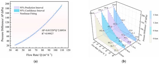
Figure 7.
Flow rate–pressure difference relationship: (a) Flow rate–pressure difference relationship for the HAICV at a spring adjustment height of 0.6 cm. The scatter points represent measured data, including the 95% confidence interval, prediction interval, and nonlinear fit. (b) Flow rate–pressure difference relationships for the HAICV at four spring adjustment heights. The scatter points represent the measured data. The color gradient corresponds to the four spring adjustment heights, respectively.
Figure 7 shows that the head loss of the HAICV increases with the flow rate, as does the rate at which it increases. The flow exponent of the fitted curve shows that the valve’s resistance characteristics are approximately quadratic. This suggests that the internal flow regime within the HAICV is predominantly fully developed turbulence, in which local head loss dominates and results in quadratic growth of the pressure difference with flow rate. Specifically, at an inlet flow rate of around 37 m3/h, the pressure difference across the valve is 24 kPa. When the flow rate increases to around 90 m3/h, the pressure difference increases to 128 kPa, approximately five times higher than at the lower flow rate. Therefore, in irrigation control, setting the valve flow rate correctly can effectively mitigate the increase in head loss, thereby enhancing the system’s overall operational efficiency and performance.
A comparison of the flow rate–pressure difference curves for the HAICV at the four spring adjustment heights reveals that they all exhibit a similar quadratic growth trend in their flow rate–pressure difference relationships. In the low-flow range (Q < 70 m3/h) and under identical flow rate conditions, there are discernible differences in the pressure difference across the HAICV corresponding to different spring heights. The pressure difference is smallest at a height of 0.6 cm and largest at 1.5 cm. For every 1 cm increase in spring adjustment height, the pressure difference across the valve increases by approximately 4 kPa. However, in the medium-to-high flow range (Q > 70 m3/h), the differences in pressure become minor and negligible under the same flow rate. This further demonstrates that spring adjustment height primarily influences HAICV performance under low-pressure, low-flow conditions, with no effect on operation during normal irrigation scenarios.
3.1.3. Flow Coefficient and Resistance Coefficient
As the preceding results confirmed, the spring adjustment height does not affect the operation of the normal irrigation system. Therefore, the flow and resistance coefficients of the HAICV were calculated based on a spring adjustment height of 0.6 cm. The differences in the calculated results for the other three heights are negligible. The detailed calculation results are presented in Table 4.
Table 4.
The following section presents a segment of the flow coefficient and resistance coefficient data for the HAICV.
As the turbulence developed fully, the flow coefficient and resistance coefficient of the HAICV fluctuated within the ranges of 78.27–80.10 and 16.35–17.12, respectively. However, these fluctuations remained relatively stable overall, as demonstrated in Figure 8. This result indicates that in the fully developed turbulent regime, the turbulent boundary layer thickness, separation bubble length, and wake vortex scale essentially cease to change with further increases in the Reynolds number. Consequently, the flow and resistance coefficients remain largely constant, which aligns with the conclusions presented in references [7,51] that these coefficients maintain constant values in high Reynolds number flows. The minor fluctuations observed (a maximum relative deviation of 2.3% for the flow coefficient and 4.7% for the resistance coefficient) are primarily governed by the geometric characteristics of the flow passage or originate from experimental uncertainties. Consequently, for operating conditions where the HAICV is in a fully developed turbulent state, the average values can be adopted as characteristic parameters: flow coefficient Kv = 79.26 and resistance coefficient ζ = 16.70.
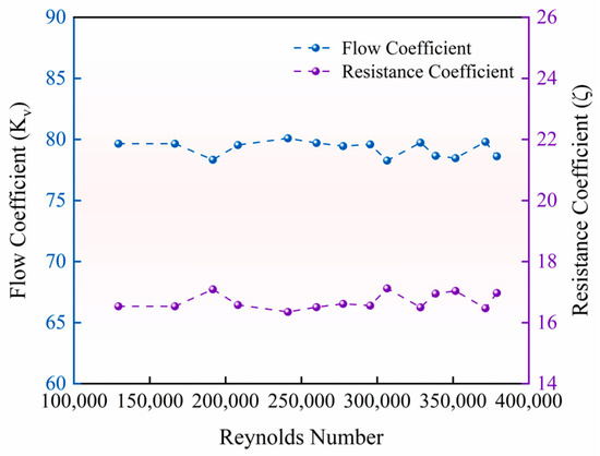
Figure 8.
Comparison of the flow coefficient and resistance coefficient for the HAICV.
Although the HAICV does not rely on electrical power or network supply, its fully mechanical structure grants it good operational reliability and long-term durability, demonstrating promising application potential and practical value. However, a comparative analysis of the hydraulic characteristics between the HAICV and common irrigation valves reveals a performance gap.
Compared with the findings for typical gate valves [41], the cited literature indicates that the flow coefficient of gate valves increases continuously over the entire opening range, with a typical value reaching 90. In contrast, the flow path design of the valve in this study is more complex, resulting in a slightly lower overall flow capacity. Furthermore, compared with ball valves [52], it is observed that the flow coefficient of a ball valve reaches its peak (approximately 96) at around 70% opening and then stabilizes, exhibiting a clear saturation characteristic. The saturated flow coefficient value of the HAICV is of the same order of magnitude as this peak value. For diaphragm valves [53], the flow coefficient is highly sensitive to the Reynolds number and can reach up to 100 at high Reynolds numbers. Regarding globe valves [54], flat-bottom globe valves exhibit relatively small flow variations with smooth and gradual regulation; trapezoidal globe valves show relatively larger flow variations, but the changes are more uniform; tapered-seat globe valves experience significant flow variations with strong regulation effects, making them prone to overshoot. The maximum flow coefficients of these three types of globe valves remain around 100. This comparative analysis indicates that, while ensuring specific functionalities, the HAICV exhibits fluid permeability intermediate among traditional control valves, while its flow resistance coefficient is generally higher than that of other common irrigation valves.
It is preliminarily inferred that the primary reason for this discrepancy lies in the more complex internal flow passage structure of the HAICV compared to conventional valves. When fluid passes through this complex passage, it generates intense impact and local vortices within the valve chamber, leading to significant energy loss. This indicates substantial potential for optimization in its internal structural design. The specific turbulent motion of the fluid within the valve chamber will be visualized through numerical simulation in the following section.
3.1.4. Uncertainty of Flow Coefficient and Resistance Coefficient
To ensure the reliability of the Type A uncertainty evaluation, this study conducted 20 independent repeated tests under identical conditions, with strict measurements of both the flow coefficient and the resistance coefficient. Through statistical analysis of each set of data, the sample variance, standard deviation, and arithmetic mean of the two coefficients were calculated, and the relevant results are summarized in Table 5.
Table 5.
Calculation of Type A uncertainty.
In contrast, Type B uncertainty primarily originates from the accuracy of the measuring instruments. From Equations (1) and (2), the various input quantities and their influence weights (sensitivity coefficients) for the flow coefficient Kv and the resistance coefficient ζ can be determined. Notably, the pipe diameter used for calculating the flow velocity is identical to the flow meter’s dimension; consequently, the relative uncertainty introduced by the flow velocity measurement is the same as that of the flow rate measurement. Specific details are provided in Table 6.
Table 6.
Calculation of the primary sources of Type B uncertainty.
The combined standard uncertainty was calculated using the root-sum-square method. For the flow coefficient, Kv, the combined relative standard uncertainty is given by:
where urel(Kv) is the relative standard uncertainty of the flow coefficient, u2Brel(qv), u2Brel(∆pv) and u2Brel(ρ) represent the sensitivities of the flow coefficient to the flow rate, pressure difference, and density, respectively.
Expanded relative uncertainty (k = 2):
Urel (Kv) = 2 × urel (Kv) = 2.276%
Absolute expanded uncertainty:
Therefore, the final result for the flow coefficient Kv of the HAICV can be expressed in the form of Equation (23):
Kv = 79.2552 ± 1.8; k = 2
Similarly, the resistance coefficient ζ for the HAICV can be determined as follows:
ζ = 16.70 ± 0.76; k = 2
The significance of the uncertainty evaluation can be interpreted as follows: there is approximately a 95% probability that the values of the HAICV’s flow coefficient and resistance coefficient lie within the intervals [77.46, 81.06] and [15.94, 17.46], respectively.
3.2. Numerical Simulation of the HAICV
To investigate the evolution of the flow field distribution characteristics in the HAICV over the opening time, numerical simulation was employed to obtain pressure and velocity nephograms within the flow domain during the opening cycle. This approach aims to reveal the evolution patterns of flow domain characteristics during the coupled motion of the flow field and the valve spool, thereby providing reference points for future structural optimization of the valve.
3.2.1. Pressure Contour Changes at Different Moments During the Opening Process
Figure 9 shows the pressure distribution on the outlet cross-section and the valve spool of the HAICV at different time instants during the opening process. Overall, the pressure in the inlet section and the valve spool is consistently higher than that in the outlet section throughout the valve opening process. The extent of the low-pressure zone in the outlet section gradually decreases as the opening degree increases, and a significant pressure gradient exists across the entire flow field region.

Figure 9.
Pressure nephograms of the outlet cross-section and valve spool of the HAICV at different time instants. Each subplot represents a cross-sectional cloud map at different moments during the activation process.
Specifically, during the initial opening stage (t ≤ 0.0125 s), the pressure in the inlet section is much lower than the weight of the valve spool assembly. The sealing area of the valve spool is subjected to the impact of the main flow, resulting in maximum pressure at this location, and the valve remains closed. Due to the minimal gap between the valve spool and the inner wall of the valve housing, and with the outlet boundary condition set to atmospheric pressure, a very small portion of the fluid forms a jet through the gap into the valve chamber, driven by the pressure difference between the high inlet pressure and the low chamber pressure. However, most of the water flow still impacts the sealing area of the valve spool, causing significant pressure accumulation in this region. This impact phenomenon is consistent with the force distribution characteristics observed by Ji [55] in the upper chamber of a high-speed switching control valve under small opening conditions, where the fluid impacts the upper chamber floor after entering it.
When the inlet pressure slightly exceeds the weight of the valve spool assembly (0.0125 s < t ≤ 0.075 s), the valve spool begins to rotate and rise, but the opening degree remains small. The incoming fluid cannot fully enter the valve spool flow passage, and the impact of the main flow on the sealing area of the valve spool weakens. The pressure drop from the valve bottom to the spool’s flow domain is relatively small at this stage, with the major pressure drop concentrated near the outlet region of the valve spool. This occurs because flow stagnation develops on the side of the valve spool top opposite the outlet, leading to significant pressure stratification between the outlet edge and the valve chamber wall. This pressure difference constitutes the main part of the pressure loss at this stage, and the flow passage is in a state of intense local throttling-stagnation coupling.
As the water pressure increased further (0.075 s ≤ t ≤ 0.125 s), the HAICV reached half opening and the coupled throttling-stagnation state weakened. This trend was similar to that reported in reference [56]. Specifically, for the ball valve described in the literature, a significant pressure gradient existed near the valve core outlet under small to medium opening conditions, resulting in peak energy loss and pressure drop. As the opening increased, the flow pattern stabilized and the flow capacity improved further. A significant pressure gradient was also observed at the outlet of the HAICV before it reached half opening. Furthermore, as the degree of opening increased, the stagnation area of the flow at the valve spool outlet gradually decreased, confirming the common flow characteristics of valves under small to medium opening conditions. The relative position of the inlet ports between the valve spool and the valve base gradually becomes more vertical, resulting in an improvement in the overall flow capacity. However, since the valve spool is not fully lifted, all four outlets of the valve housing participate in outflow, resulting in relatively high-pressure loss at this stage. Prolonged operation at this opening degree is not recommended. The pressure variation within the HAICV from inlet to outlet becomes more uniform, but the primary pressure drop remains concentrated in the outlet region of the valve spool. The pressure gradient in this throttling zone is more pronounced than in the previous stage, indicating that pressure loss is induced within the internal annular flow passage during the spool’s lifting process, accompanied by complex flow phenomena such as fluid turbulence, shear, and rotation. Local high-pressure zones appear at the bottom and top of the valve spool due to impact from the incoming flow, making these two areas critical locations prone to material wear.
When the valve enters the final stage of opening (0.125 s < t ≤ 0.1375 s), the coupled state essentially disappears. There is no flow accumulation within the flow passage, and the pressure decreases uniformly along the flow direction. As the opening degree increases, the pressure at the bottom of the valve spool decreases, and the pressure range gradually converges towards the outlet, reflecting the influence of the increased flow area on the local flow structure. At the junction between the valve spool and the inner wall of the valve housing, there exists both high-pressure fluid infiltrating through the gap and backflow from the outlet fluid impacting the valve wall. Consequently, this gap region becomes a pressure accumulation zone inside the valve, where the convergence of fluids from different sources leads to significant pressure stratification. After the HAICV is fully open (t = 0.175 s), the internal flow fully connects with the external environment, the pressure inside and outside the valve chamber stabilizes, and the entire flow field reaches a steady state. It is noteworthy that the internal pressure distribution within the valve chamber during the opening process indicates that agricultural irrigation systems utilizing the HAICV must consider the pressure-bearing capacity of the inlet section and the potential wall adsorption effects at the outlet section during the design phase.
3.2.2. Velocity Contour Changes at Different Moments During the Opening Process
Figure 10 shows the velocity distribution at the outlet and the bottom cross-section of the valve spool of the HAICV at different time instants during the opening process. Overall, the flow velocity at the valve spool and the valve housing outlet is consistently higher than that in the inlet section and the internal region of the valve spool throughout the opening process. The extent and magnitude of the high-velocity zone in the outlet section expand along the flow direction as the valve opening degree increases, indicating a gradual improvement in flow passage patency.
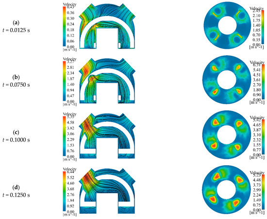
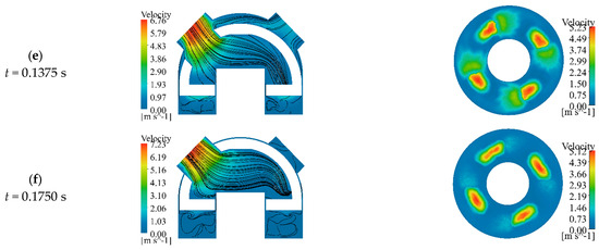
Figure 10.
Velocity nephograms of the outlet and bottom cross-section of the valve spool of the HAICV at different time instants. Each subplot represents a cross-sectional cloud map at different moments during the activation process. The left-hand figure shows the velocity contour map at the center cross-section of the outlet combined with the streamline trajectory. The figure on the right displays the velocity contour map at the bottom cross-section of the valve spool.
Specifically, during the initial opening stage (t ≤ 0.0125 s), the small opening degree results in significant flow obstruction by the valve, leading to low velocity upstream of the valve. A small amount of water injected into the valve spool experiences velocity reduction near the guide pillar surface due to viscous effects, leading to a tendency to fall back before fully developing. At this time, a very small portion of the fluid forms a high-velocity jet through the narrow gap between the valve spool and the inner wall of the valve housing. The jet velocity rapidly decays after entering the suddenly expanded valve chamber. A large low-velocity zone and secondary flow develop above the valve spool. The flow direction, influenced by wall adhesion effects, tends toward the top of the valve housing. This flow structure not only increases energy loss but also promotes particle deposition under sediment-laden conditions.
When the inlet pressure slightly exceeds the weight of the valve spool assembly (0.0125 s < t ≤ 0.075 s), the flow field inside the valve exhibits distinct velocity stratification. The high-velocity zone at the bottom of the valve spool expands, while the velocity remains lower on the side away from the outlet. The valve opening remains small at this stage, but more water flows into the interior of the valve spool. Constrained by the limited flow area, the fluid velocity increases sharply, forming a distinct banded high-velocity jet zone in the outlet section. This high-velocity jet zone disturbs the internal flow within the valve chamber, intensifying the secondary flow above the valve spool and exhibiting a noticeable vortex tendency. Simultaneously, the high velocity induces intense turbulence and wall friction, increasing the pressure difference across the valve. The passive impact on the valve spool outlet wall and the guide pillar is amplified. Combined with the effects of corners and curved surfaces, which cause the fluid to preferentially follow the curved paths, the erosion and abrasion at the top of the valve spool and guide pillar become more severe. In contrast, the flow near the junction between the valve spool and the inner wall of the valve housing relatively weakens. Han et al. [57] observed an identical phenomenon, where the fluid dissipates in the front, middle, and rear directions of the ball valve spool, forming secondary flows that impact the spool’s curved sidewall. This phenomenon is described as the merging, dispersion, and transfer of vortices.
As the opening degree further increases (0.075 s < t ≤ 0.125 s), the velocity distribution inside the valve spool becomes more uniform, the flow capacity at the inlet improves, the high-velocity zone at the bottom expands further, the overall flow area of the passage increases, and the erosion and abrasion on the valve spool are significantly reduced. The enhanced flow capacity in the outlet section raises the central velocity of the high-velocity zone, thereby expanding the banded area, and the vortices on both sides of the guide pillar gradually dissipate. However, due to a certain offset between the valve spool and the valve housing outlet, the flow distribution in the transition zone remains uneven, with some fluid constrained by the walls and concentrated closer to the downstream junction area. After passing through the outlet, the flow velocity increases, resulting in a steep velocity gradient. Entrainment effects cause the jet convergence zone to shift toward the upstream side of the outlet. Combined with wall effects, this intensifies vortex phenomena, leading to significant energy loss. The upper side of the valve spool has a large angle with the incoming flow direction, and this area still maintains a low-velocity zone. Compared to the previous stage, the overall flow conditions improve, and the velocity gradient becomes clearer.
When the valve enters the final opening stage (0.125 s < t < 0.175 s), it can be considered essentially fully open, with the velocity at the outlet reaching its maximum value. The flow rate through the valve further increases and gradually approaches a stable value. The high-velocity zone at the bottom of the valve spool reaches its maximum extent, while the blocked flow within the spool weakens. The flow tends to stabilize, and the vortex structures inside the valve spool and chamber largely disappear. As a result, the scouring effect of the water flow on the guide pillar is significantly alleviated. The high fluid velocity in the banded high-velocity zone of the outlet section causes a decrease in pressure in the inlet section, making it easier for water flow to enter the valve chamber. It is noteworthy that the valve spool has now moved to its highest position. Due to the relatively small inlet of the valve spool, not all water flow can enter the next flow passage. Consequently, a significant amount of water accumulates between the bottom of the valve spool and the valve housing base. This portion of the flow has low velocity and interacts with the continuously incoming flow, resulting in a relatively chaotic [41] flow state where vortices and collisions persist. This observation provides a feasible direction for future structural optimization of the HAICV.
In summary, the energy loss inside the valve body is primarily concentrated in the valve spool region. The fundamental reason lies in the HAICV’s use of an arc-shaped valve spool and a non-straight-through flow passage structure. After the water flow enters the valve body, internal turbulence is first generated within the arc-shaped valve spool, leading to intense momentum exchange and energy dissipation among water particles. Additionally, the continuous impact and scouring of the valve body’s inner wall and the top of the guide pillar by the water flow result in partial kinetic energy dissipation. The non-straight-through structure results in an excessively curved flow channel, forcing the water flow to undergo a significant directional adjustment before exiting. This sharp turn further increases local resistance. Coupled with the relatively small flow area at the outlet and the high flow velocity, this leads to a significant pressure drop and substantial overall energy consumption. Therefore, this valve exhibits high energy loss characteristics in practical operation, and its hydraulic performance is mainly controlled by the internal flow field structure and flow characteristics.
4. Conclusion
This study systematically analyzes the hydraulic characteristics and opening transient behavior of the HAICV. The main conclusions are as follows:
- Uncertainty analysis was introduced to define the reasonable fluctuation ranges of the flow coefficient and resistance coefficient, providing qualitative parameters for HAICV system design and practical references for the measurement of hydraulic parameters in similar valves.
- This study revealed the pressure drop concentration phenomenon and internal vortex evolution during the valve opening process, identifying the bottom and top of the valve spool as high-pressure vulnerable zones, thereby providing direction for the structural reinforcement and fatigue protection of these critical areas.
- The dynamic evolution patterns of velocity distribution characteristics under different opening degrees were clarified, revealing significant scouring phenomena on the valve spool and guide pillar during the initial opening stage, which provides theoretical support for optimizing the valve structure to enhance erosion resistance.
In summary, this study has elucidated the flow characteristics of the HAICV in the open state through a combination of physical experiments and numerical simulations. Future work should further investigate the flow transitions and water hammer effects during valve closure to ensure pipeline system safety, and undertake structural optimization based on the flow field data to reduce hydraulic losses. Particular attention should be paid to the issues of internal sedimentation and friction that may be caused by particulate matter in sediment-laden water flow. Problems such as increased opening/closing torque, as well as seal wear, can directly impact valve longevity and reliability, warranting further in-depth investigation. Furthermore, despite its characteristics of high energy consumption, the high flow resistance of the HAICV can be transformed into a regulatory advantage in the self-pressure irrigation districts of Xinjiang. It functions as a built-in pressure reducer, demonstrating significant applicability and value in this specific context.
Author Contributions
Conceptualization, M.H. and X.Y.; methodology, M.H., X.Y. and S.F.; software, M.H. and X.Y.; validation, X.Y., G.N., J.W., W.Y. and S.F.; formal analysis, M.H., X.Y. and S.F.; investigation, X.Y., G.N. and J.W.; resources, M.H. and S.F.; data curation, M.H. and X.Y.; writing—original draft preparation, M.H. and X.Y.; writing—review and editing, M.H. and X.Y.; visualization, X.Y., G.N. and J.W.; supervision, W.Y. and S.F.; project administration, M.H. and S.F.; funding acquisition, M.H. and S.F. All authors have read and agreed to the published version of the manuscript.
Funding
This research was funded by Key Research and Development Projects of the Xinjiang Uygur Autonomous Region, Science and Technology Department of Xinjiang Uygur Autonomous Region, China (2022B02011-1), the Water Resources Science and Technology Special Fund Projects of the Xinjiang Uygur Autonomous Region, Science and Technology Department of Xinjiang Uygur Autonomous Region, China (XSKJ-2023-18).
Institutional Review Board Statement
Not applicable.
Informed Consent Statement
Not applicable.
Data Availability Statement
The data presented in this study can be made available upon request from the authors. The data are not publicly available due to privacy restrictions.
Conflicts of Interest
Author Shifeng Fan was employed by the company Xinjiang Karez Irrigation Technology Co., Ltd. The remaining authors declare that the research was conducted in the absence of any commercial or financial relationships that could be construed as a potential conflict of interest.
Abbreviations
The following abbreviations are used in this manuscript:
| HAICV | Hydraulic Actuated Irrigation Control Valve |
| UDF | User-Defined Function |
| CFD | Computational Fluid Dynamics |
| VFD | Variable Frequency Drive |
| Kv | Flow coefficient |
| ζ | Resistance coefficient |
| qv | Flow rate (m3/h) |
| ρ | Mass density (kg/m3) |
| ∆pv | Pressure loss (MPa) |
| ρ0 | Mass density of pure water at 15 °C (kg/m3) |
| v | Flow velocity (m/s) |
References
- Lisowski, E.; Rajda, J. CFD Analysis of Pressure Loss During Flow by Hydraulic Directional Control Valve Constructed from Logic Valves. Energy Convers. Manag. 2013, 65, 285–291. [Google Scholar] [CrossRef]
- Lisowski, E.; Czyżycki, W.; Rajda, J. Three Dimensional CFD Analysis and Experimental Test of Flow Force Acting on the Spool of Solenoid Operated Directional Control Valve. Energy Convers. Manag. 2013, 70, 220–229. [Google Scholar] [CrossRef]
- Posa, A.; Oresta, P.; Lippolis, A. Analysis of a Directional Hydraulic Valve by a Direct Numerical Simulation using an Immersed-Boundary Method. Energy Convers. Manag. 2013, 65, 497–506. [Google Scholar] [CrossRef]
- Yu, F.W.; Xu, Y.C.; Yan, H.J. Numerical Simulation Study on Hydraulic Performance of Diaphragm Valve. Water 2025, 17, 1450. [Google Scholar] [CrossRef]
- Brazhenko, V.; Cai, J.; Fang, Y. Utilizing A Transparent Model of a Semi-Direct Acting Water Solenoid Valve to Visualize Diaphragm Displacement and Apply Resulting Data for CFD Analysis. Water 2024, 16, 3385. [Google Scholar] [CrossRef]
- Moujaes, S.F.; Jagan, R. 3D CFD Predictions and Experimental Comparisons of Pressure Drop in a Ball Valve at Different Partial Openings in Turbulent Flow. J. Energ. Eng. 2008, 134, 24–28. [Google Scholar] [CrossRef]
- Tabrizi, A.S.; Asadi, M.; Xie, G.; Lorenzini, G.; Biserni, C. Computational Fluid-Dynamics-Based Analysis of a Ball Valve Performance in the Presence of Cavitation. J. Eng. Thermophys. 2014, 23, 27–38. [Google Scholar] [CrossRef]
- Sun, X.; Kim, H.S.; Yang, S.D.; Kim, C.K.; Yoon, J.Y. Numerical Investigation of the Effect of Surface Roughness on the Flow Coefficient of an Eccentric Butterfly Valve. J. Mech. Sci. Technol. 2017, 31, 2839–2848. [Google Scholar] [CrossRef]
- Wang, D.; Bai, C.Q. The Parametric Modeling of Local Resistance and Pressure Drop in a Rotary Ball Valve. J. Fluids Eng. 2018, 140, 31204. [Google Scholar] [CrossRef]
- Nguyen, Q.K.; Jung, K.H.; Lee, G.N.; Park, S.B.; Kim, J.M.; Suh, S.B.; Lee, J. Experimental Study on Pressure Characteristics and Flow Coefficient of Butterfly Valve. Int. J. Nav. Arch. Ocean 2022, 15, 100495. [Google Scholar] [CrossRef]
- Davis, J.A.; Stewart, M. Predicting Globe Control Valve Performance—Part II: Experimental Verification. J. Fluids Eng. 2002, 124, 778–783. [Google Scholar] [CrossRef]
- Wang, Y.; Zhu, Y.; Shen, X.R.; Ma, J.F. Numerical Simulation and Experimental Research of a New Butterfly Valve. Appl. Mech. Mater. 2012, 212, 1255–1260. [Google Scholar] [CrossRef]
- Dumitrache, C.L.; Deleanu, D. Computational NX Fluid Structure Interaction (FSI) Analysis on Naval Three Way Ball Valve. IOP Conf. Ser. Mater. Sci. Eng. 2021, 1182, 012021. [Google Scholar] [CrossRef]
- Wang, H.; Cao, C.; Zhao, J.Y.; Yu, M.; Zhang, Y. Research on Dynamic Characteristics of a Novel High-Frequency Water Hydraulic Proportional Flow Valve. Flow. Meas. Instrum. 2025, 104, 102893. [Google Scholar] [CrossRef]
- Wang, Y.D.; Zheng, Z.J.; Yu, F.F.; Qian, M.; He, L. Numerical–Experimental Research on the Influence of Inclined Angle on the Flow Characteristics of Angle Seat Valve. J. Eng. 2019, 13, 168–171. [Google Scholar] [CrossRef]
- Himr, D.; Habán, V.; Hudec, M. Experimental Investigation of Check Valve Behavior During the Pump Trip. J. Phys. Conf. Ser. 2017, 813, 012054. [Google Scholar] [CrossRef]
- Zhang, Y.H.; Liu, B.; She, X.H.; Luo, Y.; Sun, Q.; Teng, L. Numerical Study on the Behavior and Design of a Novel Multistage Hydrogen Pressure-Reducing Valve. Int. J. Hydrogen Energy 2022, 47, 14646–14657. [Google Scholar] [CrossRef]
- Qian, J.Y.; Liu, B.Z.; Lei, L.N.; Zhang, H.; Lu, A.L.; Wang, J.K.; Jin, Z.J. Effects of Orifice on Pressure Difference in Pilot-Control Globe Valve by Experimental and Numerical Methods. Int. J. Hydrogen Energy 2016, 41, 18562–18570. [Google Scholar] [CrossRef]
- Yang, Y.; Zhang, Z.M.; Jia, Y.R.; Geng, T.; Xu, W.; Zhang, K. Simulation Analysis and Experimental Research on Static Performance of Water-Hydraulic Pressure Difference Control Valve. Flow Meas. Instrum. 2024, 100, 102723. [Google Scholar] [CrossRef]
- Mo, Y.T.; Zhang, C.; Jin, B.; Chen, L. Simulation and Experiment of Static and Dynamic Characteristics of Pilot-Operated Proportional Pressure Reducing Valve. Flow Meas. Instrum. 2025, 101, 102764. [Google Scholar] [CrossRef]
- Tsukiji, T. Numerical Simulation of an Unsteady Axisymmetric Flow in a Poppet Valve Using a Vortex Method. ESAIM Proc. 1997, 1, 415–427. [Google Scholar] [CrossRef][Green Version]
- Stosiak, M.; Karpenko, M.; Ivannikova, V.; Maskeliūnait, L. The Impact of Mechanical Vibrations on Pressure Pulsation, Considering the Nonlinearity of the Hydraulic Valve. J. Low Freq. Noise Vib. Act. Control. 2025, 44, 706–719. [Google Scholar] [CrossRef]
- Boyce-Erickson, G.C.; Fulbright, N.J.; Voth, J.; Chase, T.; Li, P.Y.; Ven, J. Mechanical and Hydraulic Actuation Strategies for Mainstage Spool Valves in Hydraulic Motors. In Proceedings of the ASME/BATH 2019 Symposium on Fluid Power and Motion Control, Longboat Key, FL, USA, 9 October 2019. [Google Scholar]
- Filo, G.; Lisowski, E.; Rajda, J. Flow Analysis of a Switching Valve with Innovative Poppet Head Geometry by Means of CFD Method. Flow Meas. Instrum. 2019, 70, 101643. [Google Scholar] [CrossRef]
- Wang, Z.Y.; Liu, Y.S.; Wang, X.; Liu, Y.; Pan, X.M.; Gao, C.Q.; Wu, D.F. Numerical Analysis and Experimental Verification of a Novel Water Hydraulic Rotary Proportional Valve for an Environment-Friendly Manipulator. Front. Mech. Eng. 2025, 20, 3. [Google Scholar] [CrossRef]
- Cui, B.L.; Lin, Z.; Zhu, Z.C.; Wang, H.; Ma, G. Influence of Opening and Closing Process of Ball Valve on External Performance and Internal Flow Characteristics. Exp. Therm. Fluid Sci. 2017, 80, 193–202. [Google Scholar] [CrossRef]
- Saha, B.K.; Chattopadhyay, H.; Mandal, P.B.; Gangopadhyay, T. Dynamic Simulation of a Pressure Regulating and Shut-Off Valve. Comput. Fluids 2014, 101, 233–240. [Google Scholar] [CrossRef]
- Qian, J.; Wei, L.; Jin, Z.; Wang, J.; Zhang, H.; Lu, A. CFD Analysis on the Dynamic Flow Characteristics of the Pilot-Control Globe Valve. Energy Convers. Manag. 2014, 87, 220–226. [Google Scholar] [CrossRef]
- Guo, R.; Yin, Y.B.; Li, J.; Jiang, J.L.; Fu, J.Y. The Flow Model of the Overlap Spool Valve Considering the Transition Between Laminar and Turbulent Flow. Flow Meas. Instrum. 2024, 100, 102689. [Google Scholar] [CrossRef]
- Zhang, P.; Tao, Y.; Yang, C.H.; Ma, W.N.; Zhang, Z.D. Transient Characteristics Simulation and Flow-Field Analysis of High-Pressure Pneumatic Pilot-Driven On/Off Valve Via CFD Method. Flow Meas. Instrum. 2024, 97, 102620. [Google Scholar] [CrossRef]
- Turesson, M. Dynamic Simulation of Check Valve Using CFD And Evaluation of Check Valve Model in RELAP5. Master’s Thesis, Chalmers University of Technology, Göteborg, Sweden, 2011. [Google Scholar]
- Kim, N.S.; Jeong, Y.H. An Investigation of Pressure Build-Up Effects Due to Check Valve’s Closing Characteristics Using Dynamic Mesh Techniques of CFD. Ann. Nucl. Energy 2020, 152, 107996. [Google Scholar] [CrossRef]
- Ivancu, L.; Popescu, D. Investigation of the Fluid Flow in a Large Ball Valve Designed for Natural Gas Pipelines. Appl. Sci. 2023, 13, 4247. [Google Scholar] [CrossRef]
- Hasan, A.T.; Matsuo, S.; Setoguchi, T. Characteristics of Transonic Moist Air Flows Around Butterfly Valves with Spontaneous Condensation. Propul. Power Res. 2015, 4, 72–83. [Google Scholar] [CrossRef][Green Version]
- Li, S.Y.; Wu, P.; Cao, L.L.; Wu, D.Z.; She, Y.T. CFD Simulation of Dynamic Characteristics of a Solenoid Valve for Exhaust Gas Turbocharger System. Appl. Therm. Eng. 2017, 110, 213–222. [Google Scholar] [CrossRef]
- Li, S.X.; Hou, Y.Z.; Li, L.C. Dynamic Characteristics of Swing Check Valve Based on Dynamic Mesh and UDF. Appl. Mech. Mater. 2013, 321–324, 86–89. [Google Scholar] [CrossRef]
- SolidWorks, version 2020; Software for Technical Computation; Dassault Systems: Waltham, MA, USA, 2020.
- Microsoft PowerPoint, version 2019; Software for Technical Computation; Microsoft Corporation: Redmond, WA, USA, 2019.
- Ye, Y.; Yin, C.B.; Li, X.D.; Zhou, W.J.; Yuan, F.F. Effects of Groove Shape of Notch on the Flow Characteristics of Spool Valve. Energy Convers. Manag. 2014, 86, 1091–1101. [Google Scholar] [CrossRef]
- Cheng, Y.X.; Tang, Y.; Wu, J.H.; Jin, H.; Shen, L.X. Numerical Simulation Study on Hydraulic Characteristics and Wear of Eccentric Semi-Ball Valve under Sediment Laden Water Flow. Sustainability 2024, 16, 7266. [Google Scholar] [CrossRef]
- Lin, Z.; Ma, G.F.; Cui, B.L.; Li, Y.; Zhu, Z.C.; Tong, N. Influence of Flashboard Location on Flow Resistance Properties and Internal Features of Gate Valve Under the Variable Condition. J. Nat. Gas Sci. Eng. 2016, 33, 108–117. [Google Scholar] [CrossRef]
- Raisee, M.; Alemi, H.; Iacovides, H. Prediction of Developing Turbulent Flow in 90°-Curved Ducts Using Linear and Non-Linear Low-Re K–Ε Models. Int. J. Numer. Methods Fluids 2010, 51, 1379–1405. [Google Scholar] [CrossRef]
- Chen, L. Uncertainty Assessment of Valve Flow Coefficient and Flow Resistance Coefficient Measurements. China Insp. Body Lab. 2016, 24, 36–39. (In Chinese) [Google Scholar]
- Ansys Fluent, version 2024 R1; Software for Technical Computation. ANSYS, Inc: Canonsburg, PA, USA, 2024.
- Chen, C.; Zhao, Y.Y.; Liu, J.P.; Zhao, Y.X.; Hussain, Z.; Xie, R.J. Numerical Simulation of the Flow Field Stabilization of a Pressure-Regulating Device. Agriculture 2024, 14, 1873. [Google Scholar] [CrossRef]
- Song, X.G.; Cui, L.; Cao, M.S.; Cao, W.P.; Park, Y.C.; Dempster, W.M. A CFD Analysis of the Dynamics of a Direct-Operated Safety Relief Valve Mounted on a Pressure Vessel. Energy Convers. Manag. 2014, 81, 407–419. [Google Scholar] [CrossRef]
- Liu, Y.; Bai, M.J.; Zhang, K.; Zhang, B.Z.; Li, Y.N.; Wang, Y.P.; Liu, J.T.; Liu, H.R.; He, Y.T. Study on the Impact of Pipe Installation Height on the Hydraulic Performance of Combined Canal–Pipe Water Conveyance Systems. Agriculture 2025, 15, 1347. [Google Scholar] [CrossRef]
- Launder, B.E.; Spalding, D.B. The Numerical Computation of Turbulent Flows. Comput. Methods Appl. Mech. Eng. 1974, 3, 269–289. [Google Scholar] [CrossRef]
- Qian, J.Y.; Gao, Z.X.; Wang, J.K.; Jin, Z.J. Experimental and Numerical Analysis of Spring Stiffness on Flow and Valve Core Movement in Pilot Control Globe Valve. Int. J. Hydrogen Energy 2017, 42, 17192–17201. [Google Scholar] [CrossRef]
- Alimonti, C. Experimental Characterization of Globe and Gate Valves in Vertical Gas–Liquid Flows. Exp. Therm. Fluid Sci. 2014, 54, 259–266. [Google Scholar] [CrossRef]
- Valdés, J.R.; Rodríguez, J.M.; Saumell, J.; Pütz, T. A methodology for the parametric modelling of the flow coefficients and flow rate in hydraulic valves. Energy Convers. Manag. 2014, 88, 598–611. [Google Scholar] [CrossRef]
- Lin, Z.; Wang, D.R.; Tao, J.Y.; Zhu, Z.C.; Guo, X.M. Transient Regulating Characteristics of V-Port Ball Valve in Opening and Closing Process. J. Fluids Eng. 2022, 144, 101201. [Google Scholar] [CrossRef]
- Liu, Y.N.; Lu, L.; Zhu, K.W. Numerical Analysis of the Diaphragm Valve Throttling Characteristics. Processes 2019, 7, 671. [Google Scholar] [CrossRef]
- Cui, B.L.; Ma, G.F.; Wang, H.J.; Lin, Z.; Shang, Z. Influence of Valve Core Structure on Flow Resistance Characteristics and Internal Flow Field of Throttling Stop Valve. J. Mech. Eng. 2015, 51, 178–184. (In Chinese) [Google Scholar] [CrossRef]
- Ji, H.X.; Han, J.Z.; Wang, Y.; Wang, Q.X.; Yang, S.; Xie, Y.D.; Song, Y.L.; Wang, H.B. Numerical Study on the Internal Flow Field Characteristics of a Novel High-Speed Switching Control Valve. Actuators 2024, 13, 213. [Google Scholar] [CrossRef]
- Lin, Z.H.; Li, J.Y.; Jin, Z.H.; Qian, J.Y. Fluid Dynamic Analysis of Liquefied Natural Gas Flow Through a Cryogenic Ball Valve in Liquefied Natural Gas Receiving Stations. Energy 2021, 226, 120376. [Google Scholar] [CrossRef]
- Han, Y.; Zhou, L.; Bai, L.; Xue, P.; Lv, W.N.; Shi, W.D.; Huang, G.Y. Transient Simulation and Experiment Validation on the Opening and Closing Process of a Ball Valve. Nucl. Eng. Technol. 2022, 54, 1674–1685. [Google Scholar] [CrossRef]
Disclaimer/Publisher’s Note: The statements, opinions and data contained in all publications are solely those of the individual author(s) and contributor(s) and not of MDPI and/or the editor(s). MDPI and/or the editor(s) disclaim responsibility for any injury to people or property resulting from any ideas, methods, instructions or products referred to in the content. |
© 2025 by the authors. Licensee MDPI, Basel, Switzerland. This article is an open access article distributed under the terms and conditions of the Creative Commons Attribution (CC BY) license (https://creativecommons.org/licenses/by/4.0/).