Novel Model for Pork Supply Prediction in China Based on Modified Self-Organizing Migrating Algorithm

Abstract

Pork supply prediction is a challenging task of significant importance for pig producers and administrators, as it aids decision-making and maintains the pork supply–demand balance. Previous studies failed to consider impact factors like the month-age transfer principle of pigs, epidemic factors, and the simultaneous import and export volumes of pork, leading to the absence of a quantitative prediction model for pork supply. In this background, we proposed a novel quantitative prediction model of pork supply that incorporates pork production and pork import/export volumes. First, a prediction model for pork production that takes into account the month-age transfer principle of pigs and epidemic factors was presented, along with a recursive model of the pig-herd system. A novel method based on a modified self-organizing migrating algorithm (MSOMA) was proposed for calculating the quantity of monthly newly retained sows (NRS). Furthermore, the pork-production prediction model considered the epidemic factor as a random disturbance term (RDT), and a prediction method based on MSOMA and a back-propagation neural network (MSOMA-BPNN) was introduced to predict such disturbance terms. Second, the proposed MSOMA-BPNN was employed to predict pork import and export volumes. The pork supply was subsequently determined based on the predicted pork production, as well as the pork import and export volumes. The proposed pork supply prediction model was applied to forecast China’s pork supply from 2010 to 2023. The results validate the high effectiveness and reliability of the proposed model, providing valuable insights for decision makers. The empirical results demonstrate that the proposed model is a promising and effective tool for predicting the pork supply. To our knowledge, this is a novel tool for pork supply prediction, considering the pig-herd system and pork import and export volumes from a systemic perspective. These features allow for consideration of the scientific formulation of a pig production plan, the establishment of early warning mechanisms to deal with epidemic situations and emergencies, and the regulation of pork supply and demand balance.

1. Introduction

China, the most populated country in the world, plays a major role in both consuming and producing pork. According to the national consumption structure, pork accounts for 63.45% of total meat consumption. The recent decrease in pork supply and the significant fluctuations in pork prices have garnered considerable attention from various stakeholders [1]. Specifically, the advent of COVID-19 in early 2020 and the emergence of African swine fever (ASF) in 2018 have substantially reduced pork production in recent years. For different stakeholders in the pork supply chain, farmers and pork processing enterprises face the risks of reduced production and rising raw material costs, but they also benefit from the income increase brought by the rise in pork prices. Retailers and consumers face the risk of rising purchase costs; the government needs to take measures to ensure a stable supply in the pork market, stabilize pork prices, and strive to maximize social welfare. Pork demand has remained relatively stable, resulting in an imbalance between supply and demand, causing higher and more volatile pork prices. Therefore, it is critical to make precise pork supply forecasts in order to ensure consistent production and availability of live pigs, as well as steady pork supply and prices. The forecasting of pork supply is not just a systemic concern for the entire swine industry but also a socio-economic concern linked to people’s well-being. Furthermore, ensuring a stable pork supply plays a crucial role in achieving food security, improving nutrition, and promoting the healthy and sustainable development of agricultural production and meat supply chains. A scientifically reliable pork supply prediction system also aligns with the zero-hunger goal proposed by the United Nations for Sustainable Development.

Recent research has yielded fruitful results in the study of live pigs, pork prices, and pork supply. In terms of the research on live pigs and pork prices, Hamulczuk and Stańko [2] suggested that pork prices in Poland are determined by the supply–demand balance and conducted an empirical analysis to support this claim. Alexakis et al. [3] highlighted the significant influence of pig production costs on pig price fluctuations. Ngarava and Mushunje [4] employed multiple linear regression analysis to examine the pricing strategies adopted by the pork industry in Zimbabwe. Pourmoayed and Nielsen [5] proposed a two-level Markov decision process utilizing the information on pork price, piglet price, and feed price and used a Bayesian method to analyze the optimal strategy in various price fluctuation scenarios. Zhu et al. [6] introduced a novel model to predict hog prices in China. However, the model does not take into account the impact of ASF outbreaks. Xiang et al. [7] used the back-propagation neural network (BPNN) model to predict short-term and medium-term fluctuations in pork prices. Sun et al. [8] utilized ARCH family and BVAR models to study pork price fluctuations in China during the ASF epidemic. Wang [9] developed an information technology-based short-term forecasting model for the price theory of agricultural products in the Chinese market.

In terms of the research on predicting pork supply, Jensen et al. [10] suggested in their research that the population size of breeding sows influences the production capacity of piglets. The breeding-sow inventory directly reflects pig producers’ previous investment decisions. Liang et al. [11] developed a prediction model for China’s annual live pig supply by considering five key factors. Wang et al. [12] referred to the research findings of Jensen et al. [10] and employed the principles of discrete population prediction modeling to establish a prediction model for a discrete pig population. This method faces challenges in addressing practical production issues. Nonetheless, it offers novel ideas and methodologies for further research on the pig-herd system. Jeremic et al. [13] employed the cobweb model to analyze the pork market in Serbia, and pork price was identified as a crucial factor affecting pork supply. Zhang and Wang [14] utilized a population prediction model to predict the pork supply in Heilongjiang Province of China. Accounting for the impact of ASF in 2018 and COVID-19 in early 2020 remains unknown in terms of the model’s predictive capability. Wang et al. [15] put forward a prediction model for pork supply, which incorporates an improved mayfly optimization algorithm and BPNN. The model directly forecasts the future pork supply based on historical data without considering the month-age transfer principle of pigs. This limitation hampers the formulation of effective future pig-production plans. With a specific emphasis on the matter concerning the quantity of newly retained sows (NRS), Song et al. [16] developed a prediction model for this matter using the pig month-age transfer principle and random disturbance terms. Their successful predictions established a solid groundwork for forecasting pork supply.

Although scholars have achieved fruitful research results, the previous studies on pork prediction still face the following challenges.

• The previous pork-prediction methods were investigated using the established research theories and methodologies, neglecting to account for the growth characteristics of pigs, namely, the principle of month-age transfer. As a result, they can only analyze the past changes in pigs and pork, lacking the ability to scientifically predict future pig numbers and pork supply at a specific time;
• To forecast the future pork supply, it is necessary to obtain the initial condition of different varieties of pigs within the pig herd during the preceding prediction stage, which serves as the foundation for recursion. The initial state information of the pig system includes the number of newborn piglets, sow herd, boar herd, and hog herd. However, there is no complete record of the initial condition of the pig herd in the statistical data, and the information is unknown, making it difficult to accurately predict the future pork supply;
• The method for determining the quantity of NRS is a key component of the proposed pork supply prediction model. Although a method for estimating the quantity of NRS has been given in the literature [16], the assumption that the quantity of NRS is proportional to pork prices has limitations. In fact, the quantity of NRS will not increase indefinitely with the increase in pork prices. Pig breeders are rational, and the government will take certain interventions and regulatory measures to improve this situation;
• There is a scarcity of quantitative studies on pork supply prediction, and the models that have been used so far fail to simultaneously consider the principle of month-age transfer of pigs, the influence of epidemic factors, and the pork import/export volume on pork supply.

Against this backdrop, we attempt to propose a new quantitative prediction method for pork supply. Given the remarkable success of metaheuristic algorithms in various domains, such as engineering optimization problems [17], medical research [18], and production scheduling [19], we aim to investigate the effectiveness of metaheuristic approaches for determining the model parameters of our proposed pork supply prediction model. The self-organizing migrating algorithm (SOMA) is a stochastic optimization algorithm introduced by Zelinka and Lampinen [20] that draws inspiration from the self-organizing characteristics exhibited by groups within a social setting. Numerous algorithm versions, including the discrete self-organizing migrating algorithm (DSOMA) [21], the hybrid self-organizing migrating algorithm (HSOMA) [22], and the self-adapting self-organizing migrating algorithm (SASOMA) [23], have demonstrated the higher optimization accuracy and faster convergence speed of SOMA. It has found applications in inventory-optimization problems [24], path planning [25,26], physics [27], and other fields, showing promising prospects. However, these versions of SOMA are not considered final. When confronted with complex optimization problems, SOMA still has the problems of unreasonable parameter setting, slow convergence speed, and poor solution quality. Moreover, many practical applications require algorithms to be more efficient and capable of solving problems faster and with more accuracy. Therefore, considering the specific problems at hand, this paper proposes a new version of SOMA called the modified self-organizing migrating algorithm (MSOMA) based on the SOMA team-to-team adaptive (SOMA T3A) [28], so as to make up for the drawbacks of SOMA T3A and promote the accuracy of the pork supply prediction model.

Expanding upon the analysis previously mentioned, this paper introduces an innovative prediction model of pork supply utilizing MSOMA. The primary novelty and contributions of this work are as follows.

• An innovative quantitative prediction model considering multiple influencing factors was proposed rather than the qualitative analysis in the existing research. The proposed model simultaneously considers the principle of a pig’s month-age transfer, epidemic factors, and the import and export volumes of pork;
• A nonlinear method for determining the quantity of NRS was proposed. This nonlinear method better considers the specific characteristics of production practice rather than simply setting a linear proportional relationship between the number of NRS and pork prices. The model parameters were estimated using MSOMA, which allowed for a precise estimation of the quantity of NRS;
• The proposed model takes into account the impact of epidemic factors on the pig-herd system and pork supply. The epidemic factor was introduced into the pork supply prediction model as random disturbance terms (RDTs), and a prediction method based on MSOMA and a back-propagation neural network (MSOMA-BPNN) was introduced to predict such RDTs;
• The import and export volume of pork is a major factor affecting the total pork supply, which is ignored in the previous research. The proposed pork supply prediction model considered the pork import and export volumes, and the proposed MSOMA-BPNN was employed to forecast these volumes;
• The proposed pork supply prediction model was employed to predict China’s pork supply, and the results verified the effectiveness and reliability of the proposed model. On this basis, China’s pork supply in 2023 was predicted, and the corresponding suggestions were provided in a targeted manner.

The remaining sections of this paper are structured as follows. Section 2 describes the pork supply prediction model. Section 3 provides forecasts for China’s pork supply, and Section 4 offers conclusions. Appendix B Table A8 contains a complete listing of frequently mentioned abbreviations and definitions pertinent to this paper.

2. Pork Supply Prediction Model

As a major global pork importer, China’s pork supply prediction should encompass both pork production and import/export volumes. This section presents the prediction model for pork production and the prediction model for pork import and export volumes. Finally, the prediction method and steps for pork supply are provided.

2.1. Pork-Production Prediction

In this subsection, first, the month-age recursive model of the pig-herd system is deduced. Second, since the core issue in pig-herd recursion is determining the quantity of NRS, a nonlinear model is designed to tackle this issue. An MSOMA-based approach is introduced to solve the model parameters. Third, the epidemic factor is introduced into the pork-production prediction model as RDTs, and a method for adjusting the RDTs is provided, along with a proposed model based on MSOMA-BPNN for the prediction of RDTs. Finally, the pork-production model, parameter settings, and data sources are presented.

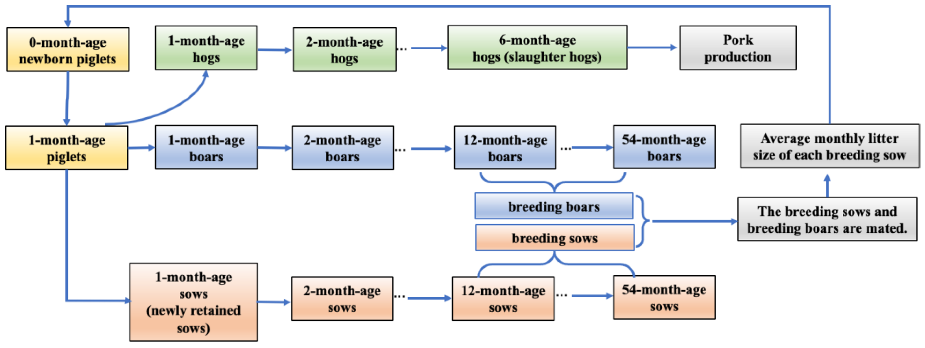
2.1.1. Recursive Model of Pig-Herd System

In production practices, pigs undergo various growth phases throughout their life cycle. These stages are typically divided into months based on the pig’s age. Consequently, the month-age transfer of pigs is the procedure by which pigs transition from one growth stage to another. This paper uses the month age as the smallest time unit to accurately estimate the quantity of each category in the pig system.

According to the different roles and production functions, the pig herd is categorized into four groups, namely newborn piglets, sows, boars, and hogs. For the convenience of understanding and expression, we first provide the definitions of various categories of pigs in the pig-herd system as follows.

• Definitions:

Newborn piglets (NP)—Live piglets produced by breeding sows.

Sows—The retained female pigs for farrowing. Its maximum utilization age is 54 months of age.

Newly retained sows (NRS)—When newborn piglets reach one month of age, they are artificially kept as breeding sows based on market conditions.

Breeding sows (BS)—Sows grow to 12 months of age, acquire reproductive ability, and become breeding sows.

Boars—The male pigs that have not been castrated are used for mating with multiple sows in the pig herd. Its maximum utilization age is 54 months of age.

Breeding boars (BB)—The boars that can continue to breed normally after their first mating at 12 months of age.

Hogs—The pigs are kept from the pig herd to provide pork after slaughter.

Slaughtered hogs (SH)—6-month-age hogs that can be slaughtered to provide pork.

Based on the research [16], the concept of month-age transfer for pigs can be understood in the following ways: 0-month-age piglets mature into 1-month-age piglets after one month, further classified into 1-month-age NRSs, hogs, and boars. Six-month-age hogs are slaughtered in order to supply pork for the market. Twelve-month-age sows mature into BSs after a period of twelve months, whereas boars of the same age mature into BBs. Boars and sows that have reached the age of 54 months are removed from the system after 54 months. The process of month-age transfer for the pig herd is depicted in Figure 1.

Figure 1. The month-age transfer of pigs.

Subsequently, the relationship between different categories of pigs and the recursive model for month-age transfer can be obtained. The mathematical description is as follows.

When the monthly pig count is based on the month, specifically the quantity of sows that are full r month age but younger than (r + 1) month age at time t is denoted as $z_r^W$(t), and the reproductive interval for BSs is defined as [r₁, r₂]. Then, the minimum age r₁ and maximum age r₂ of BSs are typically 12 and 54 months, respectively.

First, the quantity of piglets at 1 month age and less than 2 month age z₁(t) can be calculated using Equations (1)–(3).

$$z_{00}(t)=A\lambda (t){\displaystyle \sum _{r=r_1}^{r_2}{h}_r}(t)z_r^W(t)$$

(1)

$$z_0(t)=z_{00}(t-1)\left(1-D_{00}\right)$$

(2)

$$z_1(t)=z_0(t-1)\left(1-D_0\right)$$

(3)

where A represents the average number of piglets per litter produced by breeding sows; λ(t) represents the average number of litters per sow in the monthly breeding interval of t month; and h_r(t) denotes the reproductive mode of BS at the r-month-age at the t-th month. z₀(t) is the quantity of piglets aged below one month at the t-th month NP. D₀₀ represents the sum of mortality and elimination rate (SMER) of NPs, and D₀ represents the SMER for piglets younger than one month. The specific derivation process of Equations (1)–(3) can be found in Appendix A.

Second, the quantitative relationship between sows, boars, and hogs is as follows:

$$z_1^W(t)=k{z}_1^M(t)$$

(4)

$$z_1^M(t)=z_1^W(t)/k$$

(5)

$$z_1^R(t)=z_1(t)-z_1^W(t)-z_1^M(t)$$

(6)

where $z_1^W$(t) denotes the quantity of 1-month-age sows retained in NP; $z_1^M$(t) denotes the quantity of 1-month-age boars retained in NP; $z_1^R$(t) denotes the quantity of 1-month-age hogs retained in NP; and k represents the ratio coefficient of sows and boars retained in NP at the 1-month-age.

Finally, according to the age-recursive population model of the discrete population prediction model [14], the age-recursive pig-herd model is constructed as follows:

$$z_{r+1}^W(t+1)=z_r^W(t)(1-D_r^W)\hspace{1em}r=0,1,2,\cdots ,r_2-1$$

(7)

$$z_{r+1}^M(t+1)=z_r^M(t)(1-D_r^M)\hspace{1em}r=0,1,2,\cdots ,r_3-1$$

(8)

$$z_{r+1}^R(t+1)=z_r^R(t)(1-D_r^R)\hspace{1em}r=0,1,2,\cdots ,r_4-1$$

(9)

where $z_{r+1}^W$(t + 1), $z_{r+1}^M$(t + 1), and $z_{r+1}^R$(t + 1), respectively, represent the quantity of sows, boars, and hogs at (r + 1) month age in the (t + 1)-th month. $z_r^W$(t), $z_r^M$(t), and $z_r^R$(t), respectively, represent the quantity of sows, boars, and hogs at r month age in the t-th month. $D_r^W$, $D_r^M$, and $D_r^R$, respectively, represent the SMER of r-month-age sows, boars, and hogs. r₂, r_3, and r₄, respectively, represent the maximum age of sows, boars, and hogs. These formulas represent the quantity status of sows, boars, and hogs at r + 1 months of age after death and elimination from r months of age, namely, the process of month-age transfer.

Based on the age-recursive pig-herd model, accurately calculating the quantity of NRS emerges as the core challenge for pork-production prediction. After determining the quantity of NRS, the quantity of monthly BS is determined by applying the principle of month-age transfer. Finally, the monthly and annual pork productions are predicted using the formula for pig status. We will provide a method for determining the quantity of NRS in Section 2.1.2.

2.1.2. Method for Determining the Quantity of NRS

Given the limited availability of statistical data on the quantity of NRS, it is crucial to design a scientific and effective method for accurately determining this quantity to ensure precise pork-production prediction.

• Model Assumptions

According to the fundamental principles of market economics, the correlation between the quantity of NRSs and pork prices exhibits nonlinear characteristics. Therefore, the following hypothesis is posited:

Hypothesis: 

Pork prices and the quantity of NRSs have a nonlinear relationship.

Subsequently, the relationship model between them can be expressed in Equation (10).

$$Z_1^W(t,T)=a\times P{(t,T)}^3+b\times P{(t,T)}^2+c\times P(t,T)+d\hspace{1em}t=1,2,\cdots ,12;T=1,2,\cdots ,n$$

(10)

In Equation (10), for the t-th month of the T-th year, $Z_1^W$(t,T) is the quantity of NRSs, and P(t,T) is the pork price. a, b, c, and d are the model parameters, and the data on pork prices are available.

The nonlinear relationship between the quantity of NRSs and pork prices is consistent with the actual production situation, and its rationality and reasons are as follows.

(1) Nonlinear characteristics of market supply and demand.

Rapid response during the initial price increase: High pork prices allow farmers to reduce the payback period, and therefore, the replacement rate is higher. The growth in this stage may be relatively rapid, showing a quadratic acceleration characteristic.

Slow growth caused by market saturation: As the quantity of NRS increases, the market gradually approaches saturation. Even if pork prices continue to rise, the growth rate of NRS will slow down, as further increases in production may lead to oversupply.

Reverse adjustment under supersaturation: Pork prices do not continuously rise, and they actually decline after reaching a certain threshold. Low pork prices dampen people’s motivation to engage in pig farming, resulting in a reduction in the quantity of NRSs. This reverse adjustment is unique to the cubic term and reflects the nonlinear response of the market in an oversaturated state.

(2) Nonlinear changes in consumer behavior.

The rise in pork prices may lead to nonlinear changes in consumer behavior, such as when the price exceeds a certain threshold. Consumers may significantly reduce their pork consumption and instead seek alternatives, which will also affect the number of NRSs.

Consequently, using a cubic polynomial to describe the relationship between the quantity of NRS and pork prices can better capture the complexity of the real market, consider nonlinear characteristics such as consumer behavior, and provide more effective decision support for pig farmers and policymakers;

2.

Parameter estimation method

Given that the statistical data include fundamental information on pork prices and BSs at the end of each year, a mathematical model for parameter estimation is formulated, with the objective function being the minimum sum of squared errors between the actual and predicted values of BSs over the years. By optimizing this objective function, the unknown parameters in Equation (10) are determined.

According to the principle of month-age transfer of pigs, the BSs at the end of the (T + 1)-th year are divided into three components. The first component consists of the BSs remaining from the previous year after accounting for one year of mortality and elimination. The second component corresponds to the NRSs from February to December of the T-th year that transition into breeding sows. The third component represents the NRSs from the first month of the (T + 1)-th year that develop into breeding sows. Therefore, the formula for the quantity of BSs at the end of the (T + 1)-th year is derived as

$$\begin{array}{c}{\widehat{Z}}_N(T+1)=Z_N(T)(1-D_N^W)+{\displaystyle \sum _{t=2}^{12}\left[Z_1^W(t,T){\displaystyle \prod _{r=1}^{24-t}(1-D_r^W)}\right]}+\\ Z_1^W(1,T+1){\displaystyle \prod _{r=1}^{11}(1-D_r^W)},T=1,2,\cdots ,n\end{array}$$

(11)

where ${\widehat{Z}}_N(T+1)$ is predicted values of BSs at the end of the (T + 1)-th year, Z_N(T + 1) is the actual value of BSs at the end of the (T + 1)-th year, Z_N(T) represents the quantity of BSs at the end of the T-th year, $D_N^W$ is the total yearly SMER of breeding sows, and $D_r^W$ represents the SMER of r-month-age sows.

Let Q(T + 1) be the error between the actual value and the predicted value and substitute Equation (10) into Equation (11). We can obtain a new model to solve the unknown parameters. The model aims to minimize the sum of squared errors between the actual and predicted values of the breeding sows, as illustrated in Equation (12).

$$\begin{array}{c}{Q(T+1)= \{Z_N(T+1)-{\widehat{Z}}_N(T+1)\}}^2\\ =\{Z_N(T+1)-Z_N(T)(1-D_N^W)+{\displaystyle \sum _{t=2}^{12}\left\{\left[a\times P{(t,T)}^3+b\times P{(t,T)}^2+c\times P(t,T)+d\right]{\displaystyle \prod _{r=1}^{24-t}(1-D_r^W)}\right\}}\\ +\left[a\times P{(t,T+1)}^3+b\times P{(t,T+1)}^2+c\times P(t,T+1)+d\right]{\displaystyle \prod _{r=1}^{11}(1-D_r^W)}{\}}^2\end{array}$$

(12)

Equation (12) is an unconstrained nonlinear optimization problem with many parameters and a complex solution. This paper presents a modified self-organizing migrating algorithm (MSOMA) for solving the parameters in Equation (12);

3.

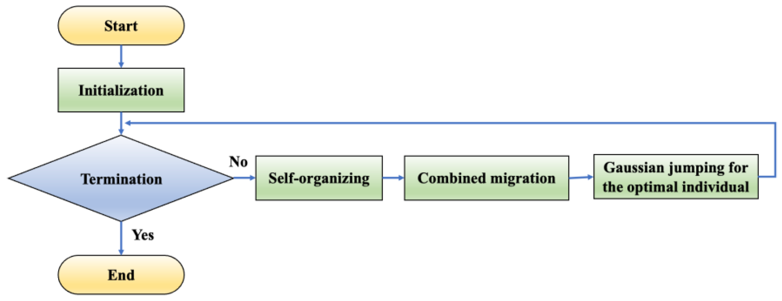
The solving method of parameter estimation model

In 2020, Diep et al. [28] introduced SOMA T3A, which achieves excellent performance in solving 100-dimensional problems. However, SOMA T3A still faces challenges, such as unreasonable parameter settings and slow convergence speed. To address these shortcomings of SOMA T3A, we propose a modified self-organized migrating algorithm (MSOMA), based on SOMA T3A. MSOMA mainly consists of four steps, namely initialization, self-organizing, combined migrating, and Gaussian jumping for the optimal individual, as shown in Figure 2. The flowchart of MSOMA is as follows:

Figure 2. The flowchart of MSOMA.

MSOMA adopts a random initialization method [16], and its main operations are as follows.

(1)

Self-organizing

The way of organization determines which individuals are migrants and which individuals become possible leaders in the population. MSOMA follows the organization approach of SOMA T3A, namely, randomly choosing a subset of m individuals from the population, and then selecting the top n individuals from that subset to be migrants. The method employs a random selection process to choose a leader for each migrant. It begins by randomly selecting a small group of k individuals from the population, and subsequently designates the individual with the highest performance as the leader. The self-organizing process is depicted in Figure 3.

Figure 3. The process of self-organizing.

The self-organizing process efficiently maintains a balance between the algorithm’s exploration and exploitation capabilities. For large values of m, n, and k, the algorithm focuses on searching in the vicinity of the current best solution, leading to local exploitation. Conversely, when their values are small, the algorithm emphasizes exploration;

(2)

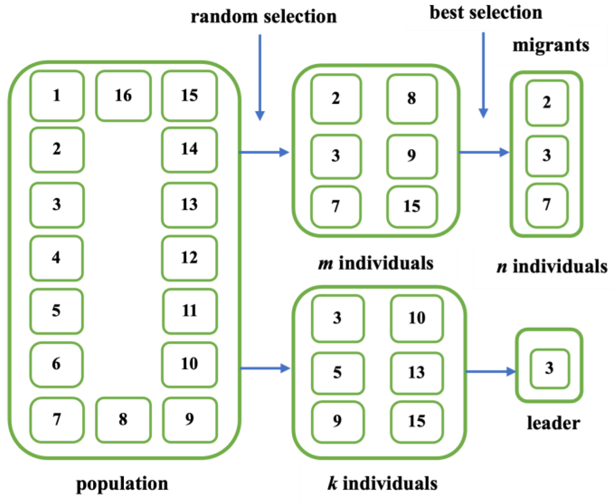
Combined migration strategy.

In SOMA T3A, a single migration strategy is utilized, which reduces the likelihood of being stuck in the local optima. However, it results in slow convergence. Additionally, the migration step (Step) and the perturbation parameter (PRT) in SOMA T3A are dynamically adaptive, which improves the algorithm’s performance compared to fixed parameters. To maintain a proper balance between global and local search capabilities, a combined migration strategy is proposed, and adaptive adjustment methods for Step and PRT are given. The combined migration strategy consists of two migration strategies, and the two mutation strategies each have a 50% probability of being executed.

The first migration strategy is an improved form of the SOMA T3A migration strategy, and its migrating method is shown in Equation (13).

$$x_i^{migrating+1}=x_i^{migrating}+\left(x_{leader}-x_i^{migrating}\right)\times Step\times PRTVevtor$$

(13)

where $x_i^{migrating+1}$ is the individual after migration and $x_i^{migrating}$ is the individual to be migrated. x_leader is the optimal individual selected from k individuals.

The value of Step determines the distance traveled by each migrating individual. To account for both exploration and exploitation throughout the iteration process, a calculation formula for adaptive dynamic adjustment of the Step value is proposed below:

$$Step=2\times (0.02+0.005\times 2\times (1.5-{\displaystyle \frac{runtime}{Maxruntime}}))$$

(14)

where rand is a random number evenly distributed between [0, 1], runtime refers to the current runtime of a program’s execution, and Maxruntime is the maximum allowable duration for the program to run. The Step value decreases as the running time increases. In the initial phases of the iterative process, the algorithm exhibits a robust capacity for exploration, as evidenced by the substantial Step value. On the contrary, as the iteration progresses, the Step value diminishes, signifying a heightened capacity for exploitation.

PRTVector is a perturbation vector that determines the moving direction of the migrating individual with each movement. The value method for each dimension in PRTVector is as follows:

$$PRTVector=\left\{\begin{array}{l}1,\hspace{1em}rand<PRT\\ 0,\hspace{1em}otherwise\end{array}\right. , PRT=0.01+0.9\times {\displaystyle \frac{runtime}{Maxruntime}}$$

(15)

where the PRT value determines the value of each component in the disturbance vector PRTVector. In the initial iteration, the PRT value is relatively small, resulting in a high probability for each component of PRTVector to take the value zero, thereby enhancing the algorithm’s capability to search globally. As the iteration progresses, the PRT value becomes large, increasing the likelihood for each component in the PRTVector to take the value of one, thereby strengthening the algorithm’s local search ability. Hence, the improved method for calculating the PRT value attains a more optimal equilibrium between the algorithm’s exploration and exploitation capabilities.

The second migration strategy cancels the limitation of perturbation vector PRTVector on the migration direction and exhibits a relatively balanced capability for both global and local searches. The migration strategy is presented in Equation (16).

$$x_i^{migrating+1}=x_i^{migrating}+\left(x_{Gbest}-x_i^{migrating}\right)\times Step\times \left(0.5\times rand\left(1,D\right)\right)+rand\left(1,D\right)\otimes \left(x_j-x_k\right)$$

(16)

where $x_{1i}^{migrating+}$ is the individual after migration and $x_i^{migrating}$ is the individual to be migrated. x_Gbest is the global optimal individual in the population, and x_j and x_k are individuals selected from the population that are different from $x_i^{migrating}$. D is the dimension of variables.

The calculation method of Step is shown in Equation (14). The second component of the migration strategy outlined in Equation (16) relies on the guidance of the optimal individual in the population, which accelerates the convergence speed of the algorithm. The third component demonstrates robust global exploration capabilities and mitigates the probability of the algorithm becoming stuck in local optimal solutions. As a result, the migration strategy maintains a relatively balanced capability for both global and local searches;

(3)

Gaussian jumping for the optimal individual

In SOMA T3A, the optimal individual x_Gbest remains unchanged during the t-th iteration, which easily leads to the algorithm being confined to a local extremum in the early stage of optimization and affects the algorithm’s performance. Therefore, to address this issue, we propose Gaussian jumping for the optimal individual x_Gbest, which generates 50 new individuals that obey the standard normal distribution near the optimal individual x_Gbest, as depicted in Equation (17).

$$x_{new\_Gbest}=N(x_{Gbest},50,1)$$

(17)

where x_Gbest is the optimal individual in the population, and x_new__Gbest is the individual generated after Gaussian jumping.

The newly generated 50 individuals are compared with the x_Gbest, and the individual with the smallest fitness value is selected as the optimal individual and participates in the (t + 1)-th iteration. The Gaussian jumping of the optimal individual helps the algorithm escape from local optima and improves the solution quality of the algorithm when performing more detailed fine-tuning.

As an example of minimizing a problem, the pseudo-code of MSOMA is provided in Algorithm 1.

Algorithm 1: The pseudo-code of MSOMA

1: Start

2: Randomly initialize the population and parameters, and evaluate the fitness function value of the individual;

3:     While runtime < Maxruntime do

4:         Update the values of Step and PRT with Equations (14) and (15), and generate a random number R between [0, 1].

5:         Select m individuals randomly from the population;

6:         Select the best n Migrants out of m individuals;

7:         For i = 1to n Migrants

8:                 Select k individuals randomly from the population;

9:                 Select the leader from k individuals;

10:                 If R < 0.5

11:                         Perform migrating strategy with Equation (13);

12:                 else

13:                         Perform migrating strategy with Equation (16);

14:             End

15:             Evaluate the fitness value and update the better position of the migrant;

16:         End For

17:         Perform Gaussian jumping of the optimal individual with Equation (17);

18:     End While

19:     Output the optimal result;

20:     End

2.1.3. Prediction of RDTs Based on MSOMA-BPNN

To reduce the effects of epidemic-related factors on pork production, the prediction model incorporates RDTs and adjusts the SMER using RDTs to enhance the prediction accuracy.

• Adjustment method based on RDTs

Taking the adjustment of BS at the end of each year as an example, the adjustment method based on RDTs is described as follows.

The relative error between the actual value and the predicted value of BS at the end of each year is used as an RDT, as shown in Equation (18).

$$\Delta (T)={\displaystyle \frac{Z(T)-\widehat{Z}(T)}{Z(T)}}\hspace{1em}T=1,2,\cdots ,n$$

(18)

where Z(T) is the actual value of BS in the T-th year, $\widehat{Z}(T)$ is the predicted value of BS in the T-th year, and $\Delta (T)$ is the RDT of the T-th year.

The RDT is employed to adjust the SMER of monthly breeding sows. Since the SMER of BSs in each month is the average value, the mortality rate of BSs in the epidemic year is higher compared to the normal year, which easily leads to the high predicted breeding sows. Therefore, the prediction accuracy of the quantity of BSs can be improved by adjusting the sows through the RDT. The specific adjustment methods are outlined as follows.

During an epidemic outbreak, the mortality rate of BSs is high. So the SMER is increased, and the adjustment method is given in Equation (19).

$$D_r^W(t)=D_r^W(t)\times (1+\Delta (T))\hspace{1em}T=1,2,\cdots ,n$$

(19)

Normal years have a low breeding-sow mortality rate, so we should reduce the SMER. The adjustment method is given in Equation (20).

$$D_r^W(t)=D_r^W(t)\times (1-\Delta (T))\hspace{1em}T=1,2,\cdots ,n$$

(20)

where $\Delta (T)$ is the RDT in the T-th year.

Similarly, in the proposed prediction model, the SMER of hogs and the monthly average litter size of each breeding sow are also adjusted by the method of RDT;

2.

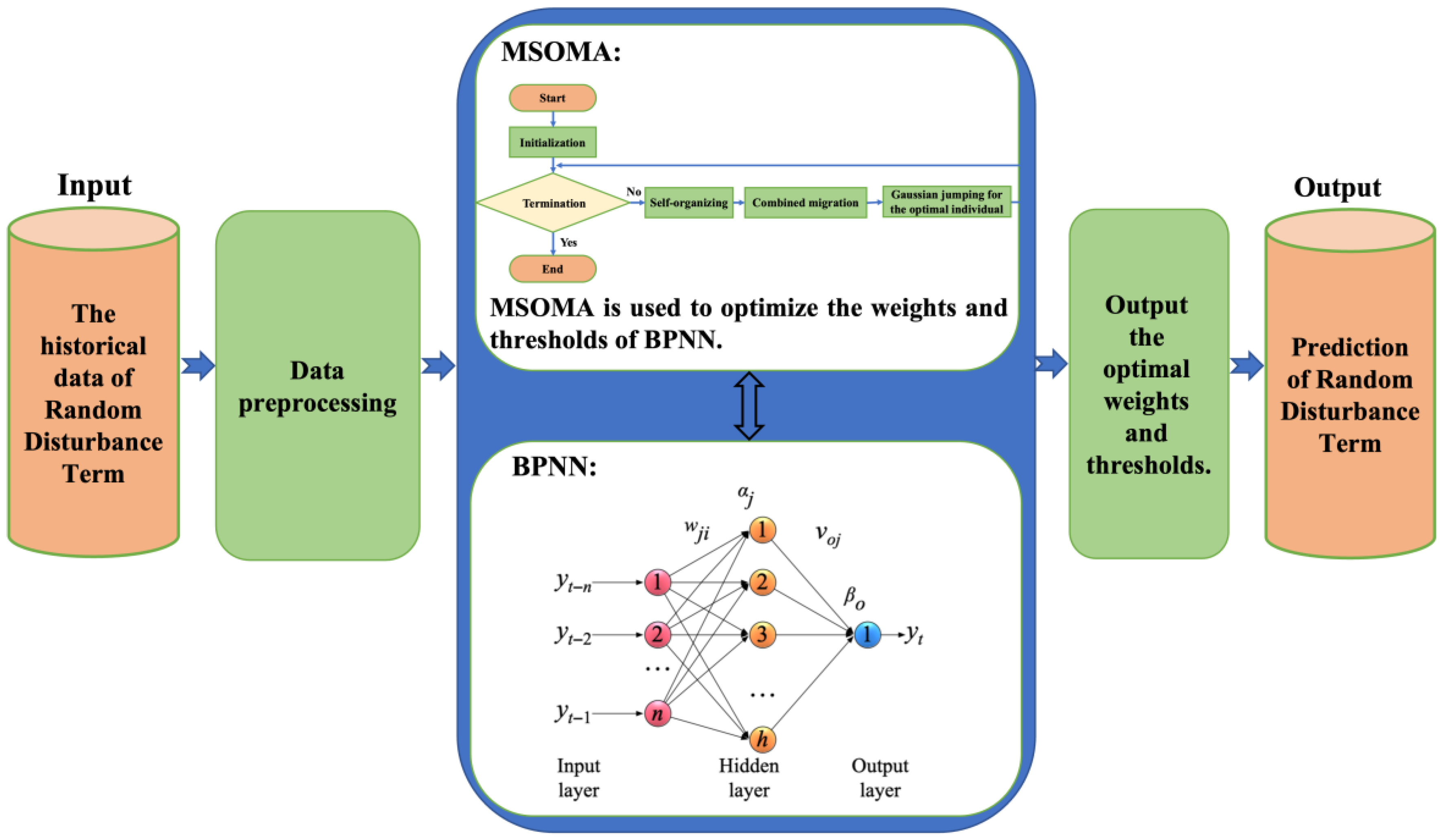
RDTs prediction method using MSOMA-BPNN

Since the influence of the annual RDT on the quantity of pigs is unknown, a quantitative recursive formula cannot be derived. Therefore, the back-propagation neural network (BPNN) can be employed for predicting the RDT, and intelligent optimization algorithms, such as genetic algorithm [29], sparrow search algorithm [30], and improved cuckoo optimization algorithm [31], were used to optimize the weights and thresholds of BPNN to improve prediction accuracy. In this paper, MSOMA is employed to optimize the weights and thresholds of BPNN. For convenience of description, the algorithm for optimizing the weights and thresholds in BPNN with MSOMA is recorded as MSOMA-BPNN, and the MSOMA-BPNN model is used to predict the RDT. The theoretical derivation of BPNN can be referenced in the literature [15,32].

Referring to Equation (18), the value of RDT from the preceding T-year is obtained and subsequently utilized as the sample data for MSOMA-BPNN. The formula utilized to perform normalization on the sample data is:

$$\Delta \prime (T)={\mathrm{l}}_1+(l_2-l_1)\left({\displaystyle \frac{\Delta (T)-{\Delta }^{\min }}{{\Delta }^{\max }-{\Delta }^{\min }}}\right)\hspace{1em}T=1,2,\cdots ,n$$

(21)

where $\Delta (T)$ is the sample data for the T-th year, $\Delta \prime (T)$ denotes the normalized sample data, ${\Delta }^{\max }$ and ${\Delta }^{\min }$ are the maximum and minimum values in the sample data, and l₁ and l₂ are the lower and upper bounds of the data processing interval, usually l₁ = −0.8, l₂ = 0.8. The normalized sample data, represented as a time series (T = 1, 2, …, n), can be forecasted using BPNN.

The process of using MSOMA-BPNN to predict RDTs is presented in Figure 4.

Figure 4. The structure of MSOMA-BPNN for the prediction of RDTs.

As can be seen from Figure 4, the process of MSOMA-BPNN predicting RDT is as follows. First, the RDTs of the previous year $\Delta (T)(T=1,2,\dots ,n)$ are calculated according to Equation (18) and used as sample data. Next, the sample data are normalized using Equation (21). Third, the normalized sample data are fitted using MSOMA-BPNN, and the optimal BPNN weights and thresholds can be determined. Finally, the RDTs are predicted using the trained BPNN.

2.1.4. Pork-Production Prediction Model

According to the age-recursive pig-herd model described in Section 2.1.1, the quantity of monthly NRSs can be calculated according to pork prices, and then the quantity of monthly BSs can be determined. Consequently, the initial condition of other categories within the pig herd can be estimated, and finally, the pork production in each month of each year can be obtained. Considering the t-th month as the reference month, the initial states for different categories of pigs at each month-age in the t-th month are outlined in Table 1.

Table 1. The initial states for different categories of pigs at each month-age in the t-th month.

NP	Sows herd
$z_{00}(t)=A\lambda (t){\displaystyle \sum _{r=r_1}^{r_2}{h}_r}(t)z_r^W(t)$ $z_0(t)=z_{00}(t)(1-D_{00})$ $z_1(t)=z_0(t-1)\left(1-D_0\right)$	$\begin{array}{l}{Z}^W(t)=\left[\begin{array}{l}{z}_1^W(t)\\ z_2^W(t)\\ z_3^W(t)\\ \cdots \\ z_{12}^W(t)\\ z_{13}^W(t)\\ \cdots \\ z_{54}^W(t)\end{array}\right]=\left[\begin{array}{l}a\times P{(t)}^3+b\times P{(t)}^2+c\times P(t)+d\\ z_1^W(t-1){\displaystyle \prod _{r=1}^1(1-D_r^W)}\\ z_1^W(t-2){\displaystyle \prod _{r=1}^2(1-D_r^W)}\\ \cdots \\ z_1^W(t-11){\displaystyle \prod _{r=1}^{11}(1-D_r^W)}\\ z_1^W(t-12){\displaystyle \prod _{r=1}^{12}(1-D_r^W)}\\ \cdots \\ z_1^W(t-53){\displaystyle \prod _{r=1}^{53}(1-D_r^W)}\end{array}\right]\\ \end{array}$
(22)	(23)
Boars herd	Hogs herd
$\begin{array}{l}{Z}^M(t)=\left[\begin{array}{l}{z}_1^M(t)\\ z_2^M(t)\\ z_3^M(t)\\ \cdots \\ z_{12}^M(t)\\ z_{13}^M(t)\\ \cdots \\ z_{54}^M(t)\end{array}\right]=\left[\begin{array}{l}{z}_1^W(t)/k\\ z_1^M(t-1){\displaystyle \prod _{r=1}^1(1-D_r^M)}\\ z_1^M(t-2){\displaystyle \prod _{r=1}^2(1-D_r^M)}\\ \cdots \\ z_1^M(t-11){\displaystyle \prod _{r=1}^{11}(1-D_r^M)}\\ z_1^M(t-12){\displaystyle \prod _{r=1}^{12}(1-D_r^M)}\\ \cdots \\ z_1^M(t-53){\displaystyle \prod _{r=1}^{53}(1-D_r^M)}\end{array}\right]\\ \end{array}$	$Z^R(t)=\left[\begin{array}{l}{z}_1^R(t)\\ z_2^R(t)\\ z_3^R(t)\\ z_4^R(t)\\ z_5^R(t)\\ z_6^R(t)\end{array}\right]=\left[\begin{array}{l}{z}_1(t)-z_1^W(t)-z_1^M(t)\\ z_1^R(t-1){\displaystyle \prod _{r=1}^1(1-D_r^R)}\\ z_1^R(t-2){\displaystyle \prod _{r=1}^2(1-D_r^R)}\\ z_1^R(t-3){\displaystyle \prod _{r=1}^3(1-D_r^R)}\\ z_1^R(t-4){\displaystyle \prod _{r=1}^4(1-D_r^R)}\\ z_1^R(t-5){\displaystyle \prod _{r=1}^5(1-D_r^R)}\end{array}\right]$
(24)	(25)

Table 1. The initial states for different categories of pigs at each month-age in the t-th month.

NP	Sows herd
$z_{00}(t)=A\lambda (t){\displaystyle \sum _{r=r_1}^{r_2}{h}_r}(t)z_r^W(t)$ $z_0(t)=z_{00}(t)(1-D_{00})$ $z_1(t)=z_0(t-1)\left(1-D_0\right)$	$\begin{array}{l}{Z}^W(t)=\left[\begin{array}{l}{z}_1^W(t)\\ z_2^W(t)\\ z_3^W(t)\\ \cdots \\ z_{12}^W(t)\\ z_{13}^W(t)\\ \cdots \\ z_{54}^W(t)\end{array}\right]=\left[\begin{array}{l}a\times P{(t)}^3+b\times P{(t)}^2+c\times P(t)+d\\ z_1^W(t-1){\displaystyle \prod _{r=1}^1(1-D_r^W)}\\ z_1^W(t-2){\displaystyle \prod _{r=1}^2(1-D_r^W)}\\ \cdots \\ z_1^W(t-11){\displaystyle \prod _{r=1}^{11}(1-D_r^W)}\\ z_1^W(t-12){\displaystyle \prod _{r=1}^{12}(1-D_r^W)}\\ \cdots \\ z_1^W(t-53){\displaystyle \prod _{r=1}^{53}(1-D_r^W)}\end{array}\right]\\ \end{array}$
(22)	(23)
Boars herd	Hogs herd
$\begin{array}{l}{Z}^M(t)=\left[\begin{array}{l}{z}_1^M(t)\\ z_2^M(t)\\ z_3^M(t)\\ \cdots \\ z_{12}^M(t)\\ z_{13}^M(t)\\ \cdots \\ z_{54}^M(t)\end{array}\right]=\left[\begin{array}{l}{z}_1^W(t)/k\\ z_1^M(t-1){\displaystyle \prod _{r=1}^1(1-D_r^M)}\\ z_1^M(t-2){\displaystyle \prod _{r=1}^2(1-D_r^M)}\\ \cdots \\ z_1^M(t-11){\displaystyle \prod _{r=1}^{11}(1-D_r^M)}\\ z_1^M(t-12){\displaystyle \prod _{r=1}^{12}(1-D_r^M)}\\ \cdots \\ z_1^M(t-53){\displaystyle \prod _{r=1}^{53}(1-D_r^M)}\end{array}\right]\\ \end{array}$	$Z^R(t)=\left[\begin{array}{l}{z}_1^R(t)\\ z_2^R(t)\\ z_3^R(t)\\ z_4^R(t)\\ z_5^R(t)\\ z_6^R(t)\end{array}\right]=\left[\begin{array}{l}{z}_1(t)-z_1^W(t)-z_1^M(t)\\ z_1^R(t-1){\displaystyle \prod _{r=1}^1(1-D_r^R)}\\ z_1^R(t-2){\displaystyle \prod _{r=1}^2(1-D_r^R)}\\ z_1^R(t-3){\displaystyle \prod _{r=1}^3(1-D_r^R)}\\ z_1^R(t-4){\displaystyle \prod _{r=1}^4(1-D_r^R)}\\ z_1^R(t-5){\displaystyle \prod _{r=1}^5(1-D_r^R)}\end{array}\right]$
(24)	(25)

The hogs are all slaughtered at 6 months of age. Assuming that each hog produces c kilograms of meat, the pork production Z(t) in the t-th month is:

$$Z(t)=c\cdot z_6^R(t)$$

(26)

Assuming a prediction period of 12 months, since the newly retained sow is a 1-month-age sow, the breeding sow is a sow from 12 months to 54 months old, and the breeding boar is a boar from 12 months to 54 months old. In order to avoid duplicate calculations, the categories of the pig-herd system are classified as newborn piglets, sows, boars, and hogs. The newborn piglet is 1 month age, the sow and boar are within the age range of [1, 54], and the hog is within the age range of [1, 6]. According to the calculation method in references [33,34], using a three-dimensional matrix to represent the dimensions of each category (animal category, month age, time horizon), the dimension of the pig-herd model is (newborn piglets, 1, 12) + (sows, 54, 12) + (boars, 54, 12) + (hogs, 54, 12) = 1 × 12 + 54 × 12 + 54 × 12 + 6 × 12 = 1380.

So far, the formulas for the initial state of pigs have been derived based on the principle of the discrete population model and the perspective of system engineering.

2.2. Prediction Model of Pork Import and Export Volumes

China is a major global pork importer, and the import and export volumes of pork significantly influence the pork supply. Hence, predicting the pork supply necessitates considering pork imports and exports. The calculation method for annual pork production is shown in Equation (27).

Pork supply = Pork production + Pork import − Pork export

(27)

Taking the pork import and export volume over the years as a time series, the proposed MSOMA-BPNN can predict future pork import and export volumes. The annual pork supply can be determined by calculating the predicted pork production and pork import and pork export volumes according to Equation (27). Thus far, we have completed the prediction of pork supply.

2.3. Determination of Related Parameters

To predict the pork supply, we require specific parameters and fundamental data. Some parameters are indirectly determined through expert research and the relevant literature, while others are directly obtained by consulting statistical data. The determination methods for the parameters obtained indirectly are as follows.

• The SMER of pigs

Based on empirical evidence and expert opinion, the annual SMER of boars and sows is 40%. The SMER of pigs at each month age in the herd system is presented in Appendix B Table A1, Table A2 and Table A3. Note that the SMER provided by statistical data is the average level of normal years, whereas the mortality rate of live pigs increases during epidemic years. Consequently, the prediction model for pork supply employs the RDTs to adjust the SMER of live pigs, thereby enhancing prediction accuracy;

2.

Average monthly litter size of each breeding sow

After reviewing the relevant literature and consulting experts [35,36,37], the range of monthly average litter size for sows is determined to be [1.6, 2.5]. In this paper, based on the monthly average litter size of each breeding sow (1.68), the quantity of SH is adjusted according to the RDTs so as to improve the quality of pork supply prediction;

3.

The retention ratio of sows and boars

Expert consultation and data generally recommend that the ideal retention ratio of sows to boars in pig farms is 20:1, denoted as k = 20;

4.

The average pork production of each slaughtered hog

In this paper, the pork production is based on the weight after slaughter. The calculation method for the average pork yield per slaughtered hog is shown in Equation (28).

Average pork production of each slaughtered hog = pork production/SH

(28)

where the annual pork production and the quantity of SHs can be obtained in the China Statistical Yearbook.

The parameters obtained directly are as follows. The statistical data on the BS stock at the end of each year, monthly pork prices, and average pork production of each SH in China are presented in Appendix B Table A4, Table A5 and Table A6 by consulting the China Statistical Yearbook [38] and the China Animal Husbandry and Veterinary Yearbook [39]. By referring to the General Administration of Customs of the People’s Republic of China [40], China’s pork import and export volumes from 2007 to 2022 are obtained, as shown in Appendix B Table A7.

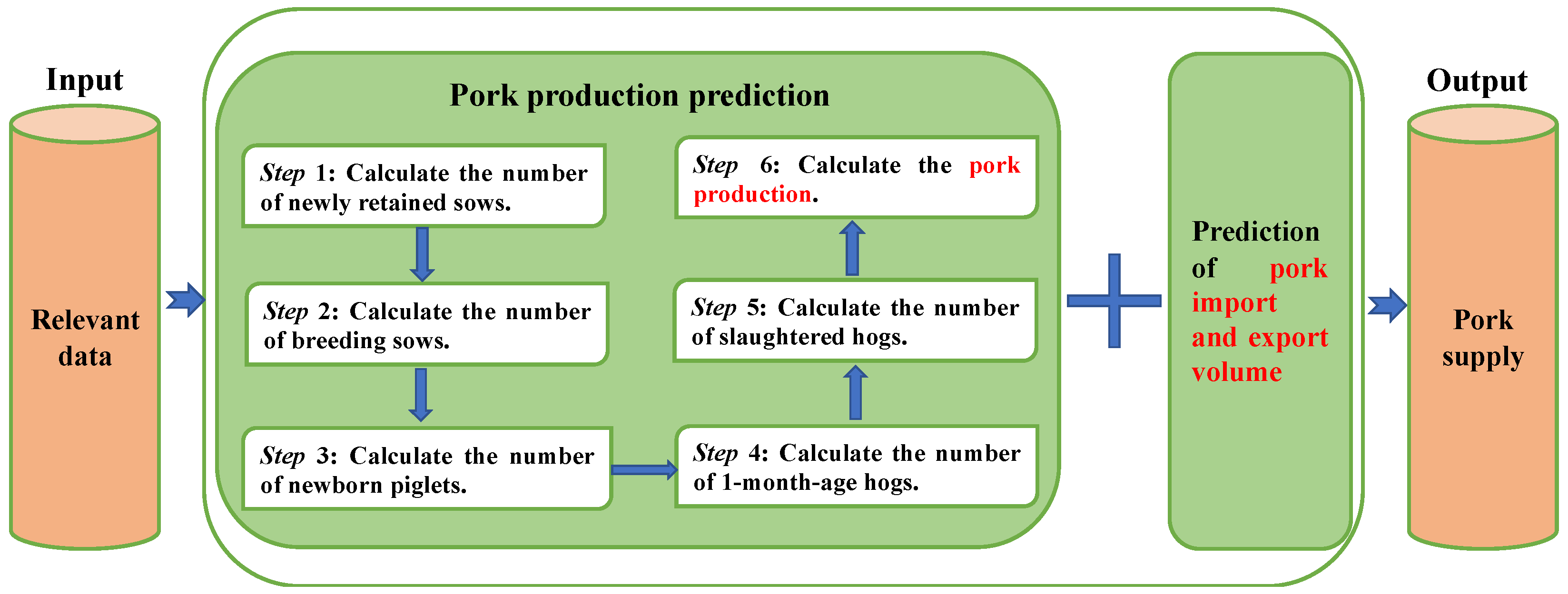
2.4. The Steps of Pork Supply Prediction

The aforementioned analysis identifies the specific steps for pork supply prediction, and Figure 5 illustrates the framework.

Figure 5. The framework of proposed pork supply prediction model.

• Input the relevant parameters into the model;
• The parameters a, b, c, and d in Equation (12) are solved by using the proposed MSOMA, and the calculation formula for the quantity of NRS can be obtained;
• Substitute the monthly pork prices into Equation (10) to obtain the quantity of NRSs in each year;
• According to the month-age transfer principle of sows in Equation (23), the quantity of monthly BSs for each year is calculated, and the RDT is predicted by the MSOMA-BPNN algorithm to adjust the quantity of monthly BS for each year;
• Determine the initial month and use it as a benchmark to estimate the quantity of monthly NP of each year using Equation (22);
• According to the quantity of monthly NRSs and the retention ratio of sows and boars, the quantity of monthly newly retained piglets can be obtained;
• Calculate the quantity of monthly SH for each year using the formula derived from Equation (25) and employ the MSOMA-BPNN algorithm to predict the RDT. Based on the RDT, adjust the SMER of hogs, as well as the monthly litter size of each breeding sow, to obtain the final number of SHs in each month;
• The historical data of the average pork production of each hog in each year is used as a time series, and MSOMA-BPNN is used to predict the average meat production of each hog. According to Equation (26), pork production can be obtained;
• In light of the import and export volumes of pork over the years, the future import and export volumes of pork are predicted using the proposed MSOMA-BPNN. On this basis, the future pork supply is predicted according to Equation (27).

3. Pork Supply Prediction for China

The effectiveness of the proposed pork supply prediction model is verified by predicting the pork supply in China, followed by a comprehensive and in-depth discussion and analysis of the results. Based on the prediction results, corresponding suggestions are provided.

3.1. Experiment Settings

The computational analyses were executed on a desktop computer equipped with a 2.40 GHz Core i5-1135G7 processor and 16 GB of RAM. MATLAB R2022a was employed for both execution and programming. In this paper, the relevant parameters of MSOMA are set to N = 1500, m = 50, n = 4, k = 100, and Njumps = 100. In MSOMA-BPNN, the mean square error (MSE) serves as the loss function, while the bipolar Sigmoid function is the activation function. In addition, we improve data quality and consistency by normalizing the data and reduce the possibility of overfitting in MSOMA-BPNN by adjusting the number of neurons and network layers in BPNN. The network is organized in a 3-5-1 configuration. When the algorithm reaches the maximum running duration, it ends the iteration. MSOMA-BPNN is executed 30 times, and the optimal result is output.

Relative error (RE) and mean relative error (MRE) were used as evaluation metrics to assess the performance of the prediction model [15]. The smaller the values of RE and MRE, the better the prediction performance.

3.2. Pork-Production Prediction for China

3.2.1. Estimation for the Quantity of NRS

The data for the quantity of BS and pork prices from 2005 to 2022 included in Appendix B Table A4 and Table A5 were substituted into Equation (12). The proposed MSOMA was utilized to solve the model parameters in Equation (12), so we can estimate the relationship between the quantity of NRS and pork prices.

The optimal parameters obtained by MSOMA are a = 0.0065934, b = −0.6354132, c = 17.9452315, and d = 57.4439554. Therefore, the relationship model between the quantity of NRS and pork prices is:

$$\begin{array}{l}{\widehat{Z}}_1^W(t,T)=0.0065934\times p{\left(t,T\right)}^3-0.6354132\times p{\left(t,T\right)}^2\\ \hspace{1em}\hspace{1em}\hspace{1em}\hspace{1em}+17.9452315\times p\left(t,T\right)+57.4439554\hspace{1em}t=1,2,\cdots ,12;T=1,2,\cdots ,n \end{array}$$

(29)

By substituting the data in Appendix B Table A4 and Table A5 into Equation (11), the predicted value of BS at the end of each year can be obtained. The values of RE and MRE between the actual value and predicted value were calculated, as presented in Table 2.

Table 2. Prediction results of the quantity of BS at the end of each year from 2006 to 2022 in China.

Year	Actual Value (Unit: 10,000 Heads)	Predicted Value (Unit: 10,000 Heads)	RE
2006	4700	4681.58	0.0039199
2007	4233.8	4535.90	−0.0713542
2008	4878.8	4409.09	0.0962763
2009	4957.7	4814.90	0.0288031
2010	4854.86	4854.86	0
2011	4911.58	4796.92	0.0233455
2012	5043.2	4784.86	0.0512248
2013	5132.3	4906.20	0.0440551
2014	4962.5	4960.81	0.0003407
2015	4693	4874.19	−0.0386096
2016	4456.2	4679.20	−0.0500429
2017	4471.5	4471.50	0
2018	4261	4550.66	−0.0679803
2019	3080.5	4451.14	−0.4449403
2020	4161.3	3657.56	0.1210545
2021	4328.7	4328.70	0
2022	4390	4392.47	−0.0005617
MRE			0.0613241

In Table 2, the value of MRE is relatively large, with a value of 0.0613241. Table 2 reveals that the ASF in 2018 and the COVID-19 epidemic in 2020 led to large fluctuations in pork production. Since the impact of the epidemic on the quantity of pigs was not considered, the predicted pork production exhibited a significant relative error. In light of the fluctuations in the SMER of pigs during the epidemic year, RDTs were implemented to mitigate the epidemic’s effect on the accuracy of predictions.

First, the RE of the previous year in Table 2 was utilized as RDTs, and the proposed MSOMA-BPNN was used to predict the time series. Because the network structure of MSOMA-BPNN is 3-5-1, the predicted RDT is from 2009 to 2022. Table 3 displays the predicted results of BS at the end of each year and RDTs.

Table 3. Prediction results for the quantity of BSs at the end of the year considering the principle of month-age transfer of pigs and the RDTs.

Year	The Quantity of Breeding Sows Based on the Pig’s Month-Age Transfer (Unit: 10,000 Heads)	RDT	The Predicted Value of Breeding Sows (Unit: 10,000 Heads)	The Actual Value of Breeding Sows (Unit: 10,000 Heads)	RE
2006	4681.58	-	-	4700	-
2007	4535.90	-	-	4233.8	-
2008	4409.09	-	-	4878.8	-
2009	4814.90	0.0288031	4953.59	4957.7	0.0008296
2010	4854.86	1.39 × 10−15	4854.86	4854.86	0
2011	4796.92	0.0233455	4908.90	4911.58	0.0005450
2012	4784.86	0.0512248	5029.97	5043.2	0.0026240
2013	4906.20	0.0440551	5122.34	5132.3	0.0019409
2014	4960.81	0.0003407	4962.50	4962.5	0.0000001
2015	4874.19	−0.0386096	4686.00	4693	0.0014907
2016	4679.20	−0.0500429	4445.04	4456.2	0.0025043
2017	4471.50	−4.82 × 10−14	4471.50	4471.5	0
2018	4550.66	−0.0679803	4241.31	4261	0.0046213
2019	4451.14	−0.4449403	2470.65	3080.5	0.1979719
2020	3657.56	0.1210545	4100.32	4161.3	0.0146542
2021	4328.70	4.44 × 10−16	4328.70	4328.7	0
2022	4392.47	−0.0005617	4390.00	4390	0.0000003
MRE					0.0162273

Table 3 reveals a close alignment between the predicted and statistical values of breeding sows, with a minimal MRE of 0.0162273 and a small deviation. This approach takes into account both the month-age transfer principle and the effect of epidemic variables on the quantity of breeding sows. As a result, the proposed approach has a high degree of accuracy. This strategy yields an effective model of the relationship between the quantity of NRS and pork prices. It is both feasible and reliable to predict the quantity of BS and pork production at the end of each year, guaranteeing the high reliability of the obtained results.

3.2.2. Prediction for the Monthly BSs

Following the prediction steps for pork supply, the quantity of monthly BSs and SHs for each year was calculated. Subsequently, the pork production was determined.

Substituting the pork prices in Appendix B Table A5 into Equation (29), we can obtain the quantity of NRS, as provided in Table 4.

Table 4. The quantity of NRSs in China from January 2005 to December 2022 (Unit: 10,000 heads).

Year	Jan	Feb	Mar	Apr	May	Jun	Jul	Aug	Sept	Oct	Nov	Dec
2005	202.79	203.52	202.03	200.47	199.09	198.54	198.16	197.55	197.83	194.52	191.95	192.40
2006	194.99	193.67	190.75	187.55	184.85	183.99	187.11	192.74	196.96	197.79	199.46	203.78
2007	205.60	205.81	204.16	203.75	208.53	212.63	215.13	214.31	214.90	215.13	214.73	213.22
2008	211.15	210.25	210.91	210.91	212.39	213.17	213.75	214.12	214.59	215.14	214.61	215.05
2009	215.12	215.11	214.50	212.40	208.02	207.37	209.61	212.95	214.22	213.95	213.67	214.34
2010	214.51	213.90	211.90	209.46	209.15	209.02	212.30	214.50	214.98	215.07	215.11	214.93
2011	214.83	214.30	214.20	213.93	213.31	209.08	203.57	202.38	201.12	202.47	206.61	208.19
2012	206.85	207.81	210.72	212.84	214.00	214.44	214.57	214.32	213.51	213.37	213.55	212.22
2013	209.60	209.80	213.30	214.89	215.08	214.42	213.89	212.36	211.37	211.60	211.86	211.64
2014	212.83	214.29	215.08	214.78	215.14	215.02	214.94	214.08	213.39	213.72	214.13	214.37
2015	214.72	214.90	215.09	215.07	214.74	214.16	211.29	206.57	205.84	207.45	209.10	209.05
2016	207.20	204.60	204.35	201.47	199.61	198.83	201.38	202.66	202.90	205.58	206.63	206.03
2017	204.39	205.25	207.71	209.31	211.62	213.15	213.28	212.82	212.08	212.29	212.59	211.80
2018	211.26	211.99	214.55	215.13	214.66	214.85	215.07	214.92	214.07	213.77	213.80	213.62
2019	214.14	214.60	213.71	212.55	212.38	211.00	206.40	192.31	178.77	192.33	218.58	194.98
2020	210.47	257.20	239.20	205.03	183.12	183.71	211.43	227.90	217.65	190.01	180.60	188.97
2021	209.32	194.07	179.88	181.17	193.76	208.51	210.03	211.31	214.07	214.70	207.63	205.60
2022	209.04	211.56	214.31	214.34	212.02	209.39	193.36	192.49	187.98	180.97	180.79	187.77

Subsequently, the quantity of monthly NRS from January 2005 to January 2021 in Table 4 was substituted into Equation (23), and the quantity of BSs of different months in the same month was summed up to obtain the quantity of BSs in each month from June 2009 to December 2022. Note that the NRSs in January 2005 will reach a 54-month age in June 2009, while those from January 2021 will reach a 12-month age in December 2021 and become breeding sows. This indicates that June 2009 is the earliest time point for calculating the quantity of breeding sows. Among them, the 54-month-age BSs are directly excluded due to their excessive age and weakened breeding function. The quantity of BSs at the end of the year was determined by the quantity of BSs in December of that year. The prediction results for the quantity of BSs in China from June 2009 to December 2022 are displayed in Table 5.

Table 5. Prediction results for BS in China from June 2009 to December 2022 (Unit: 10,000 heads).

Year	Jan	Feb	Mar	Apr	May	Jun	Jul	Aug	Sept	Oct	Nov	Dec	Predicted Values	Actual Values	RE
2009						4919.22	4927.61	4936.81	4946.89	4956.91	4967.32	4977.75	4977.75	4957.7	−0.0040439
2010	4988.23	4997.93	5007.04	5013.46	5019.08	5025.40	5034.81	5046.20	5058.41	5071.22	5084.69	5096.86	5096.86	4854.86	−0.0498463
2011	5106.15	5112.05	5115.55	5118.11	5118.84	5121.50	5125.81	5131.06	5136.46	5139.95	5141.65	5142.27	5142.27	4911.58	−0.0469693
2012	5142.78	5142.96	5142.84	5142.38	5139.11	5132.26	5124.92	5116.43	5109.19	5104.83	5101.51	5096.94	5096.94	5043.2	−0.0106566
2013	5093.09	5091.47	5091.37	5092.40	5093.60	5094.85	5095.89	5096.49	5097.78	5100.88	5103.11	5102.33	5102.33	5132.3	0.00583996
2014	5100.44	5100.90	5102.74	5104.81	5106.05	5106.78	5106.50	5106.20	5107.03	5108.18	5109.18	5109.85	5109.85	4962.5	−0.0296928
2015	5110.84	5112.26	5113.37	5114.75	5116.07	5117.35	5118.11	5118.35	5118.96	5120.11	5123.07	5128.39	5128.39	4693	−0.0927746
2016	5134.22	5140.59	5146.31	5150.06	5152.68	5153.47	5150.07	5145.02	5140.53	5137.01	5133.33	5128.18	5128.18	4456.2	−0.1507968
2017	5121.12	5114.30	5105.34	5094.97	5084.66	5077.58	5071.59	5064.54	5059.15	5054.64	5049.97	5044.28	5044.28	4471.5	−0.1280946
2018	5039.95	5038.07	5037.41	5038.52	5040.94	5042.95	5044.00	5044.13	5044.54	5045.05	5044.96	5044.47	5044.47	4261	−0.183869
2019	5044.90	5047.66	5050.70	5053.16	5055.63	5058.10	5060.34	5061.78	5062.97	5064.28	5065.65	5068.52	5068.52	3080.5	−0.6453569
2020	5073.54	5078.03	5080.89	5082.92	5083.84	5081.75	5069.36	5046.40	5035.84	5047.31	5039.90	5044.08	5044.08	4161.3	−0.2121413
2021	5085.29	5111.22	5108.18	5087.15	5067.20	5070.52	5086.71	5093.42	5077.17	5052.73	5034.87	5033.63	5033.63	4328.7	−0.1628503
2022	5020.32	4996.12	4973.29	4960.87	4960.84	4962.24	4964.35	4967.67	4971.21	4969.18	4965.48	4964.53	4964.53	4390	−0.1308725
MRE															0.13241464

Considering the impact of the epidemic on the SMER of pigs, the RE values in Table 5 served as RDTs. According to the adjustment method of the SMER in Equations (19) and (20), the quantity of BSs in China from June 2009 to December 2022 was adjusted. Table 6 lists the quantity of monthly BSs after adjustment.

Table 6. Prediction results for BS in China from June 2009 to December 2022 after adjustment (Unit: 10,000 heads).

Year	Jan	Feb	Mar	Apr	May	Jun	Jul	Aug	Sept	Oct	Nov	Dec	Predicted Values	Actual Values	RE
2009						4908.67	4917.06	4926.24	4936.30	4946.30	4956.69	4967.10	4967.10	4957.7	−0.0018961
2010	4858.46	4867.89	4876.69	4882.79	4888.10	4894.14	4903.21	4914.20	4925.96	4938.27	4951.21	4962.89	4962.89	4854.86	−0.0222524
2011	4979.46	4985.09	4988.37	4990.73	4991.35	4993.89	4998.07	5003.16	5008.39	5011.78	5013.46	5014.11	5014.11	4911.58	−0.0208743
2012	5113.38	5113.58	5113.46	5113.01	5109.74	5102.90	5095.57	5087.10	5079.87	5075.52	5072.22	5067.68	5067.68	5043.2	−0.0048534
2013	5109.20	5107.57	5107.45	5108.48	5109.68	5110.92	5111.95	5112.55	5113.84	5116.94	5119.18	5118.41	5118.41	5132.3	0.00270674
2014	5019.56	5020.05	5021.90	5023.97	5025.23	5025.98	5025.72	5025.42	5026.23	5027.35	5028.31	5028.99	5028.99	4962.5	−0.0133979
2015	4862.90	4864.37	4865.53	4866.95	4868.31	4869.62	4870.41	4870.68	4871.30	4872.44	4875.25	4880.22	4880.22	4693	−0.0398927
2016	4737.00	4742.68	4747.77	4751.12	4753.43	4753.92	4750.39	4745.40	4741.05	4737.69	4734.21	4729.32	4729.32	4456.2	−0.061289
2017	4780.32	4773.75	4765.11	4755.12	4745.17	4738.29	4732.49	4725.79	4720.78	4716.63	4712.31	4706.98	4706.98	4471.5	−0.0526624
2018	4564.07	4562.45	4562.03	4563.31	4565.82	4568.00	4569.30	4569.75	4570.45	4571.25	4571.47	4571.28	4571.28	4261	−0.0728197
2019	3588.19	3591.12	3594.30	3596.99	3599.67	3602.36	3604.84	3606.61	3608.12	3609.68	3611.20	3613.62	3613.62	3080.5	−0.1730616
2020	4533.05	4537.02	4539.51	4541.30	4542.01	4539.76	4527.56	4505.30	4494.82	4505.29	4497.68	4501.31	4501.31	4161.3	−0.0817074
2021	4660.90	4685.57	4682.35	4661.84	4642.40	4645.40	4660.84	4667.20	4651.46	4627.98	4610.97	4610.04	4610.04	4328.7	−0.0649932
2022	4677.27	4653.95	4632.03	4620.28	4620.54	4622.18	4624.54	4628.13	4631.95	4630.33	4627.09	4626.52	4626.52	4390	−0.0538777
MRE															0.0475918

It can be observed from Table 6 that the RE value of the quantity of BSs at the end of the year after adjustment is small, and the MRE value is 0.0475918, indicating the effectiveness of the prediction model for the quantity of monthly sows after considering the RDT. On this basis, improving the prediction accuracy of pork production in the next month is possible.

3.2.3. The Results of Pork Production Prediction

Following the steps for predicting pork production, the quantity of monthly NPs was calculated using Equation (22), and then the quantity of newly retained hogs and monthly SHs can be calculated using Equation (25). The results are presented in Table 7.

Table 7. Prediction results for SHs in China from 2010 to 2022 (Unit: 10,000 heads).

Year	Jan	Feb	Mar	Apr	May	Jun	Jul	Aug	Sept	Oct	Nov	Dec	Predicted Values	Actual Values	RE
2010	5434.74	5444.11	5455.87	5467.56	5478.84	5490.60	5366.84	5379.43	5391.69	5398.95	5405.14	5409.11	65122.86	66686.43	0.0234466
2011	5417.51	5429.66	5443.02	5457.07	5472.03	5485.50	5504.93	5511.46	5515.46	5518.71	5523.21	5531.06	65809.63	66326.10	0.0077869
2012	5536.91	5543.87	5548.63	5548.80	5549.31	5551.25	5663.97	5661.58	5659.55	5657.99	5653.86	5645.93	67221.66	69789.50	0.0367940
2013	5637.76	5628.80	5620.65	5615.51	5612.92	5610.07	5657.40	5652.39	5650.84	5651.85	5653.80	5655.71	67647.70	71557.30	0.0546359
2014	5658.26	5659.82	5661.09	5664.42	5667.18	5665.22	5550.82	5550.67	5553.06	5555.11	5556.65	5557.57	67299.87	73510.40	0.0844851
2015	5558.05	5558.32	5558.96	5559.87	5560.76	5561.22	5371.03	5372.54	5373.89	5375.81	5377.88	5381.95	65610.29	70825.00	0.0736280
2016	5387.09	5388.06	5387.32	5387.15	5390.41	5397.75	5236.23	5242.94	5251.34	5256.85	5260.20	5258.47	63843.81	70073.90	0.0889075
2017	5253.28	5247.36	5239.98	5235.19	5231.74	5227.62	5285.20	5275.47	5264.16	5250.66	5237.90	5229.92	62978.48	70202.10	0.1028975
2018	5223.69	5216.69	5210.76	5205.74	5201.52	5195.90	5031.74	5027.59	5026.58	5028.47	5031.18	5033.47	61433.33	69382.40	0.1145690
2019	5035.09	5036.37	5037.44	5038.33	5038.74	5038.07	3912.85	3917.01	3921.69	3924.92	3929.22	3936.43	53766.15	54419.20	0.0120003
2020	3951.90	3966.07	3955.65	3933.88	3956.78	3945.66	4955.69	4976.38	5009.88	5031.59	5031.87	5004.42	53719.76	52704.10	−0.0192711
2021	4975.69	4959.42	4972.23	4992.65	4976.42	4962.33	5158.61	5199.56	5194.70	5159.94	5124.48	5126.54	60802.57	67128.00	0.0942294
2022	5143.06	5147.87	5129.30	5108.77	5091.13	5086.98	5161.64	5132.49	5107.38	5096.02	5098.69	5114.94	61418.27	69995.00	0.1225335
MRE															0.0642450

Table 7 shows a small deviation, with an MRE value of 0.0642450 between the predicted and actual total annual SHs. However, due to the impact of epidemics, the predicted number of SHs is quite different from the actual value. As the epidemic’s impact weakens, pig production is expected to gradually return to normal in 2021. Consequently, the SMER of hogs will decrease, leading to an increase in the quantity of SHs. Therefore, the relative error in Table 7 was employed as an RDT to adjust the SMER of hogs. The adjusted number of monthly SHs is provided in Table 8.

Table 8. Prediction results for SHs from 2010 to 2022 in China after adjusting the SMER of pigs (Unit: 10,000 heads).

Year	Jan	Feb	Mar	Apr	May	Jun	Jul	Aug	Sept	Oct	Nov	Dec	Predicted Values	Actual Values	RE
2010	5455.21	5464.62	5476.41	5488.15	5499.47	5511.28	5387.05	5399.69	5412.00	5419.28	5425.50	5429.48	65368.12	66686.43	0.0197688
2011	5424.28	5436.44	5449.82	5463.89	5478.87	5492.36	5511.81	5518.35	5522.35	5525.60	5530.11	5537.97	65891.86	66326.10	0.0065470
2012	5569.66	5576.66	5581.45	5581.62	5582.13	5584.09	5697.47	5695.07	5693.03	5691.46	5687.30	5679.32	67619.28	69789.50	0.0310967
2013	5687.33	5678.29	5670.07	5664.89	5662.28	5659.40	5707.15	5702.09	5700.53	5701.54	5703.52	5705.44	68242.51	71557.30	0.0463236
2014	5735.33	5736.92	5738.20	5741.57	5744.38	5742.39	5626.43	5626.28	5628.70	5630.77	5632.34	5633.27	68216.58	73510.40	0.0720146
2015	5623.99	5624.26	5624.91	5625.83	5626.73	5627.19	5434.75	5436.27	5437.64	5439.58	5441.68	5445.80	66388.63	70825.00	0.0626385
2016	5464.33	5465.31	5464.57	5464.39	5467.70	5475.14	5311.31	5318.12	5326.64	5332.23	5335.62	5333.86	64759.21	70073.90	0.0758441
2017	5340.53	5334.51	5327.01	5322.14	5318.63	5314.44	5372.98	5363.09	5351.59	5337.86	5324.89	5316.78	64024.46	70202.10	0.0879980
2018	5320.36	5313.23	5307.19	5302.08	5297.77	5292.05	5124.85	5120.63	5119.60	5121.53	5124.28	5126.62	62570.19	69382.40	0.0981836
2019	5044.78	5046.07	5047.15	5048.04	5048.44	5047.77	3920.39	3924.55	3929.24	3932.48	3936.79	3944.01	53869.72	54419.20	0.0100972
2020	3939.70	3953.83	3943.43	3921.73	3944.56	3933.47	4940.39	4961.02	4994.42	5016.05	5016.34	4988.97	53553.91	52704.10	−0.0161242
2021	5051.33	5034.81	5047.81	5068.55	5052.07	5037.76	5237.02	5278.60	5273.67	5238.38	5202.38	5204.47	61726.85	67128.00	0.0804604
2022	5244.90	5249.81	5230.87	5209.93	5191.94	5187.71	5263.84	5234.12	5208.52	5196.93	5199.65	5216.23	62634.45	69995.00	0.1051582
MRE															0.054788

From Table 8, it can be concluded that, after adjusting the SMER, the MRE value of the annual SHs is 0.054788. However, the prediction accuracy remains unsatisfactory. Therefore, the RE values in Table 8 were used as an RDT to adjust the average monthly litter size of each breeding sow in each year and then adjust the quantity of hog stocks in each month of each year, as shown in Table 9.

Table 9. Prediction results for SHs in China from 2010 to 2022 after adjusting the monthly average litter size of BS (Unit: 10,000 heads).

Year	Jan	Feb	Mar	Apr	May	Jun	Jul	Aug	Sept	Oct	Nov	Dec	Predicted Values	Actual Values	RE
2010	5566.84	5576.46	5588.48	5600.44	5612.01	5624.05	5497.35	5510.20	5522.71	5530.14	5536.47	5540.59	66705.75	66686.43	−0.0002897
2011	5461.05	5473.30	5486.76	5500.93	5516.01	5529.58	5549.16	5555.74	5559.77	5563.03	5567.54	5575.43	66338.30	66326.10	−0.0001839
2012	5748.54	5755.72	5760.70	5760.99	5761.56	5763.54	5880.48	5878.08	5876.03	5874.45	5870.18	5861.95	69792.22	69789.50	−0.0000390
2013	5959.77	5950.28	5941.67	5936.26	5933.47	5930.35	5980.32	5975.18	5973.60	5974.67	5976.71	5978.70	71510.98	71557.30	0.0006473
2014	6162.26	6163.90	6165.29	6168.92	6171.91	6169.86	6045.65	6045.54	6048.11	6050.36	6052.03	6053.02	73296.86	73510.40	0.0029049
2015	5988.44	5988.69	5989.40	5990.40	5991.37	5991.88	5787.39	5789.02	5790.48	5792.51	5794.71	5798.93	70693.22	70825.00	0.0018607
2016	5893.03	5894.03	5893.34	5893.26	5896.81	5904.70	5728.26	5735.57	5744.54	5750.42	5754.02	5752.30	69840.27	70073.90	0.0033340
2017	5826.75	5820.22	5812.28	5807.06	5803.19	5798.50	5862.26	5851.70	5839.31	5824.57	5810.58	5801.76	69858.19	70202.10	0.0048989
2018	5861.83	5853.92	5847.31	5841.73	5836.93	5830.60	5647.05	5642.64	5641.56	5643.63	5646.68	5649.26	68943.12	69382.40	0.0063312
2019	5097.67	5098.97	5100.05	5100.95	5101.36	5100.68	3961.92	3966.12	3970.85	3974.11	3978.46	3985.71	54436.84	54419.20	−0.0003241
2020	4006.00	4020.16	4009.79	3988.12	4010.98	3999.93	5023.76	5044.46	5077.90	5099.57	5099.87	5072.46	54453.00	52704.10	−0.0331833
2021	5474.46	5455.86	5467.88	5489.60	5472.41	5458.44	5672.62	5716.50	5711.27	5674.06	5636.24	5638.62	66867.96	67128.00	0.0038738
2022	5816.78	5822.46	5801.59	5777.77	5757.69	5753.35	5837.73	5805.15	5776.86	5763.82	5766.58	5783.36	69463.15	69995.00	0.0075984
MRE															0.0050361

According to Table 9, adjusting the monthly average litter size of each breeding sow significantly improved the prediction accuracy for the annual number of SHs, as evidenced by the MRE value between the predicted and actual values of 0.0050361, with minimal deviation. This improvement is attributed to the consideration of the impact of the epidemic on pig mortality and elimination rates, in addition to the average monthly litter size of each breeding sow. Thus, the proposed prediction model is highly reliable.

After predicting the quantity of SHs in Table 9, the monthly pork production and annual total pork production were calculated using Equation (26), as presented in Table 10. The MRE value between the predicted annual total pork production and the actual value of each year is 0.0050361, indicating a small deviation. This result affirms the scientific and effective nature of the proposed pork-production prediction model.

Table 10. China’s pork-production prediction from 2010 to 2022 (Unit: 10,000 tons).

Year	Jan	Feb	Mar	Apr	May	Jun	Jul	Aug	Sept	Oct	Nov	Dec	Predicted Values	Actual Values	RE
2010	423.34	424.07	424.98	425.89	426.77	427.69	418.05	419.03	419.98	420.55	421.03	421.34	5072.71	5071.24	−0.0002897
2011	416.06	416.99	418.02	419.09	420.24	421.28	422.77	423.27	423.58	423.83	424.17	424.77	5054.06	5053.13	−0.0001839
2012	440.08	440.63	441.01	441.03	441.07	441.22	450.18	449.99	449.84	449.72	449.39	448.76	5342.91	5342.7	−0.0000390
2013	457.49	456.77	456.10	455.69	455.47	455.24	459.07	458.68	458.56	458.64	458.79	458.95	5489.44	5493	0.0006473
2014	475.42	475.55	475.66	475.94	476.17	476.01	466.43	466.42	466.62	466.79	466.92	467.00	5654.93	5671.4	0.0029049
2015	463.90	463.92	463.97	464.05	464.12	464.16	448.32	448.45	448.56	448.72	448.89	449.22	5476.29	5486.5	0.0018607
2016	445.64	445.72	445.66	445.66	445.93	446.52	433.18	433.73	434.41	434.86	435.13	435.00	5281.43	5299.1	0.0033340
2017	452.50	451.99	451.37	450.97	450.67	450.30	455.26	454.44	453.47	452.33	451.24	450.56	5425.09	5451.8	0.0048989
2018	456.54	455.92	455.41	454.97	454.60	454.10	439.81	439.46	439.38	439.54	439.78	439.98	5369.49	5403.7	0.0063312
2019	398.61	398.71	398.80	398.87	398.90	398.85	309.80	310.13	310.50	310.76	311.09	311.66	4256.68	4255.3	−0.0003241
2020	312.65	313.75	312.94	311.25	313.04	312.18	392.08	393.70	396.31	398.00	398.02	395.88	4249.79	4113.3	−0.0331833
2021	431.89	430.43	431.38	433.09	431.73	430.63	447.53	450.99	450.58	447.64	444.66	444.85	5275.38	5295.9	0.0038738
2022	460.47	460.92	459.27	457.38	455.80	455.45	462.13	459.55	457.31	456.28	456.50	457.83	5498.90	5541	0.0075984
MRE															0.0050361

So far, the prediction of pork production in China from 2010 to 2022 has been successfully accomplished. The proposed prediction method, which considers the principle of pig month-age transfer and RDTs, provides better guidance for pig breeding and establishes a foundation for effectively regulating the balance of pork supply and demand.

3.2.4. Prediction of Pork Import and Export Volumes

The import and export volumes of pork in each year were predicted using MSOMA-BPNN according to the statistical data in Appendix B Table A7. With a network structure of 3-5-1 for the MSOMA-BPNN model, the predicted pork import and export volume spans from 2010 to 2022, and the corresponding results are presented in Table 11.

Table 11. Prediction results of China’s pork import and export volumes (Unit: 10,000 tons).

Year	Actual Value of Import Volume	Predicted Value of Import Volume	RE	Actual Value of Export Volume	Predicted Value of Export Volume	RE
2007	8.6	-	-	13.36	-	-
2008	37.33	-	-	8.22	-	-
2009	13.5	-	-	7.97	-	-
2010	19.95	19.95	1.44 × 10−4	11.01	11.01	0
2011	46.77	46.77	2.22 × 10−5	8.07	8.07	0
2012	52.23	52.24	−9.73 × 10−5	6.62	6.62	0
2013	58.33	58.33	7.75 × 10−5	7.34	7.34	0
2014	56.43	56.42	1.52 × 10−4	9.15	9.15	0
2015	77.75	77.77	−2.38 × 10−4	7.15	7.15	0
2016	162.02	162.01	3.58 × 10−5	4.85	4.85	0
2017	121.68	121.68	−1.49 × 10−6	5.13	5.13	0
2018	120.1	120.10	3.38 × 10−6	4.18	4.18	0
2019	210.83	210.83	2.91 × 10−6	2.69	2.69	0
2020	439	439.00	−5.93 × 10−6	1.1	1.1	−9.08 × 10−15
2021	371.06	371.06	7.29 × 10−7	1.81	1.81	1.10 × 10−14
2022	175.79	175.79	−4.29 × 10−6	2.74	2.74	−3.57 × 10−15
MRE			7.03 × 10−6			1.82 × 10−15

From Table 11, it is evident that the MSOMA-BPNN prediction model performs well in forecasting pork import and export volumes. The MRE values in Table 11 are 7.03 × 10⁻⁶ and 1.82 × 10⁻¹⁵, respectively, and the deviation is very small, indicating that MSOMA-BPNN achieves a satisfactory prediction effect. With the trained MSOMA-BPNN model, the import and export volumes of pork in China for 2023 were predicted with high reliability.

3.2.5. Pork Supply Prediction

According to Equation (27), the prediction results of China’s pork supply from 2010 to 2022 are presented in Table 12.

Table 12. Prediction of China’s pork supply from 2010 to 2022 (Unit: 10,000 tons).

	Actual Value				Predicted Value
Year	Pork Production	Import Volume	Export Volume	Pork Supply	Pork Production	Import Volume	Export Volume	Pork Supply	RE
2010	5071.24	19.95	11.01	5080.18	5072.71	19.95	11.01	5081.65	−0.0002892
2011	5053.13	46.77	8.07	5091.83	5054.06	46.77	8.07	5092.76	−0.0001825
2012	5342.7	52.23	6.62	5388.31	5342.91	52.23	6.62	5388.52	−0.0000387
2013	5493	58.33	7.34	5543.99	5489.44	58.33	7.34	5540.43	0.0006414
2014	5671.4	56.43	9.15	5718.68	5654.93	56.43	9.15	5702.21	0.0028808
2015	5486.5	77.75	7.15	5557.1	5476.29	77.75	7.15	5546.89	0.0018370
2016	5299.1	162.02	4.85	5456.27	5281.43	162.02	4.85	5438.60	0.0032380
2017	5451.8	121.68	5.13	5568.35	5425.09	121.68	5.13	5541.64	0.0047964
2018	5403.7	120.1	4.18	5519.62	5369.49	120.10	4.18	5485.41	0.0061983
2019	4255.3	210.83	2.69	4463.44	4256.68	210.83	2.69	4464.82	−0.0003090
2020	4113.3	439	1.1	4551.2	4249.79	439.00	1.1	4687.69	−0.0299905
2021	5295.9	371.06	1.81	5665.15	5275.38	371.06	1.81	5644.63	0.0036214
2022	5541	175.79	2.74	5714.05	5498.90	175.79	2.74	5671.95	0.0073683
MRE									0.0047224

Table 12 shows that the MRE value between the pork supply obtained by the proposed pork supply prediction model and the actual value is 0.0047224, indicating a small deviation and demonstrating the effectiveness of the pork supply prediction model. The proposed model is highly reliable for predicting China’s future pork supply. Expanding on this achievement, this model was implemented to predict the pork supply in China for the year 2023.

3.3. Pork-Production Prediction for China in 2023

The pork supply prediction model was employed to predict the pork supply in China in 2023.

As the 1-month-age hogs require six months to grow into SHs, those retained from July to December 2022 influence pork production from January to June 2023, while those retained from January to June 2023 influence pork production from July to December 2023. To predict pork production in 2023, it is necessary to calculate the quantity of NRSs, breeding sows, newly retained piglets, and SHs from July 2022 to June 2023. First, the pork prices from Appendix B Table A5 for January to June 2023 were substituted into Equation (29) to obtain the quantity of NRSs during that period. Second, the quantity of monthly BSs was calculated using Equation (23), with the results presented in Table 13. Given the impact of factors like disease outbreaks on breeding-sow numbers, an RDT was added to adjust the monthly breeding-sow quantities. The RE values in Table 5 were used as the time series of RDT. The RDT in 2023 was predicted by MSOMA-BPNN, and the predicted result is −0.1837956. Then, the SMER of the monthly BSs was adjusted, with the resulting adjusted breeding-sow numbers presented in Table 13.

Table 13. The quantity of NRSs and BSs in China (Unit: 10,000 heads).

Time	NRS	Breeding Sows	BS after Adjustment
July 2022	193.36	4964.35	4624.54
August 2022	192.49	4967.67	4628.13
September 2022	187.98	4971.21	4631.95
October 2022	180.97	4969.18	4630.33
November 2022	180.79	4965.48	4627.09
December 2022	187.77	4964.53	4626.52
January 2023	202.43	4965.68	4498.75
February 2023	208.31	4969.35	4502.70
March 2023	209.32	4973.10	4506.70
April 2023	212.23	4974.91	4508.80
May 2023	212.90	4974.63	4508.89
June 2023	213.45	4961.26	4496.43

According to Equation (25) and the data in Table 13, the quantity of monthly SHs from January 2023 to December 2023 is presented in the second column of Table 14. Similarly, the RE values in Table 7 were used as the time series of RDT, and the RDT of hogs in 2023 was predicted by MSOMA-BPNN. The predicted RDT for hogs is 0.0504490, which is used to adjust the mortality and elimination rate of hogs. The resulting adjusted number of hogs is presented in the third column of Table 14. Since the average monthly litter size of each breeding sow affects the quantity of SHs, the RE values in Table 8 were used as a time series to predict the RDT of the average monthly litter size of each breeding sow in 2023. The predicted result is 0.1125191. According to the RDT, the quantity of SHs was adjusted, with the results presented in the fourth column of Table 14. Finally, the monthly pork supply was calculated based on the quantity of SH. According to the average pork production of each slaughtered hog in Appendix B Table A6, the average pork production of each slaughtered hog in 2023 was predicted, and the predicted result was 0.0793997. Equation (26) was then employed to calculate the pork production for each month in 2023, with a total annual pork production of 5421.13 thousand tons. So far, the prediction of pork production in 2023 has been completed.

Table 14. Prediction results for the quantity of SHs and pork production.

Time	SH (Unit: 10,000 Heads)	SH After Adjusting the SMER (Unit: 10,000 Heads)	SH After Adjusting Monthly Litter size Per Breeding Sow (Unit: 10,000 Heads)	Pork Production (Unit: 10,000 Tons)
January 2023	5118.42	5159.96	5760.14	457.35
February 2023	5126.57	5168.18	5768.83	458.04
March 2023	5137.22	5178.92	5780.06	458.94
April 2023	5135.54	5177.22	5778.15	458.78
May 2023	5125.57	5167.17	5767.69	457.95
June 2023	5111.77	5153.26	5753.70	456.84
July 2023	4960.31	5000.57	5584.43	443.40
August 2023	4963.92	5004.21	5588.58	443.73
September 2023	4965.88	5006.19	5591.08	443.93
October 2023	4967.69	5008.01	5593.17	444.10
November 2023	4967.30	5007.62	5592.79	444.07
December 2023	5092.99	5134.33	5717.88	454.00
Total of 2023	60673.17	61165.64	68276.50	5421.13

Finally, according to China’s import and export pork volumes in Appendix B Table A7, MSOMA-BPNN was used to predict the import and export volume of pork in 2023. The predicted import volume of pork is 192.81 thousand tons, and the export volume is 2.13 thousand tons. Based on Equation (27), China’s pork supply in 2023 is 5611.81 thousand tons.

3.4. Managerial Implications

This work also provides valuable implications for decision makers.

• A novel prediction model for pork supply was proposed. The model not only considers the principle of month-age transfer of pigs but also takes into account epidemic factors and the import/export volumes of pork. The model demonstrates high prediction quality, reliability, and an ideal prediction effect for pork supply in China. The quantity status of various types of pigs in this model can offer a scientific foundation for farmers to develop appropriate breeding strategies, production plans, and related government policies to achieve a balance between pork supply and demand;
• The proposed pork supply prediction model incorporates the impact of epidemic factors on the quantity of live pigs and adjusts the SMER of live pigs using RDTs. The RDTs have no certain rules to follow. Therefore, integrating RDTs into the pork supply prediction model can greatly enhance the accuracy of the predictions, offering a novel approach to forecasting pork supply. Furthermore, the mortality and elimination rate of pigs at various growth stages significantly affect pork production. In order to enhance the survival rate of pigs, it is recommended that relevant authorities provide comprehensive training on scientific pig-breeding knowledge and skills for pig breeders. This will facilitate the adoption of advanced breeding techniques, thereby reducing pig mortality and elimination rates during growth, as well as minimizing losses resulting from sudden epidemics. Ultimately, this will contribute to the overall advancement of the pig industry. By analyzing the fluctuations in the predicted value of RDTs, the government can implement appropriate control measures and emergency-management protocols to mitigate the impact of epidemic factors on the pig sector;
• Seeking the “alternate to port” strategy is also a promising strategy to improve the pork supply system. Since the import and export volume of pork has a significant impact on the total pork supply, decision makers can encourage the diversification of pork import and export by finding “alternate to port”, for example, finding other diverse import sources to adjust the pork supply, optimizing the logistics network, flexibly adjusting the resource allocation of different ports or supply points to reduce costs, utilizing blockchain technology to improve the transparency and efficiency of the pork supply chain, tax reduction, subsidies, simplifying import and export procedures, etc.;
• A refined version of MSOMA was suggested to address the model parameters and enhance the optimization of the weights and thresholds of BPNN, hence enhancing the accuracy of the predictions. Managers can apply this algorithm to optimize and predict similar large-scale and complex problems. Additionally, managers can customize different meta-heuristic algorithms based on their specific requirements, enhancing the adaptability and quality of the algorithm for solving similar problems.

The managerial insights obtained in this work not only furnish policymakers and pig farms in China with practical guidelines but also offer suggestions for stakeholders in other epidemic-stricken nations.

4. Conclusions

This work presents a quantitative forecast model for pork supply based on MSOMA, which simultaneously incorporates the concept of month-age transfer, epidemic variables, and the impact of the pork import and export volume. First, the recursive model of the pig-herd system was constructed and derived. To tackle the fundamental concern of ascertaining the quantity of monthly NRSs, an innovative approach utilizing MSOMA was presented. Secondly, the epidemic factor was incorporated into the pork-production prediction model as RDTs. The RDTs adjustment method for pork-production prediction was provided, and MSOMA-BPNN was introduced to predict the RDTs. Third, considering the pork import and export volumes, the MSOMA-BPNN model was employed to predict the pork import and export volumes. The pork supply was then predicted according to the predicted pork production and pork import and export volumes. Finally, the proposed model was applied to forecast the pork supply in China. The results demonstrate the high accuracy and effectiveness of the proposed pork supply prediction model. Based on these findings, China’s pork supply in 2023 was predicted, and relevant management suggestions were given.

In future work, it is worthwhile to explore the establishment of a pork supply–demand balance regulation model. Additionally, the optimal combination of MSOMA parameters can be further explored. The proposed MSOMA can be applied to solve other similar problems and can also be tailored for specific problems to enhance the algorithm’s performance.

References

- Pang, J.; Yin, J.; Lu, G.C.; Li, S.M. Supply and Demand Changes, Pig Epidemic Shocks, and Pork Price Fluctuations: An Empirical Study Based on an SVAR Model. Sustainability 2023, 15, 13130. [Google Scholar] [CrossRef]
- Hamulczuk, M.; Stańko, S. Factors affecting changes in prices and farmers’ incomes on the Polish pig market. Probl. Agric. Econ./Zagadnienia Ekon. Rolnej 2014, 4, 135–157. [Google Scholar] [CrossRef]
- Alexakis, C.; Bagnarosa, G.; Dowling, M. Do cointegrated commodities bubble together? The case of hog, corn, and soybean. Financ. Res. Lett. 2017, 23, 96–102. [Google Scholar] [CrossRef]
- Ngarava, S.; Mushunje, A. Pricing Strategies in Pork-based Agribusinesses: Evidence from Zimbabwe. S. Afr. Bus. Rev. 2019, 23, 24. [Google Scholar] [CrossRef]
- Pourmoayed, R.; Nielsen, L.R. Optimizing pig marketing decisions under price fluctuations. Ann. Oper. Res. 2022, 314, 617–644. [Google Scholar] [CrossRef]
- Zhu, H.M.; Xu, R.; Deng, H.Y. A novel STL-based hybrid model for forecasting hog price in China. Comput. Electron. Agr. 2022, 198, 15. [Google Scholar] [CrossRef]
- Xiang, C.L.; Hu, M.L.; Du, Y.; Zheng, R.Z.; Gao, J.L.; Wang, C.; Gu, L.C. Pork price forecasting based on public opinion and policy impact. J. Nonlinear Convex A 2022, 23, 1967–1978. [Google Scholar]
- Sun, D.; Chen, L.; Bu, R. Study on the Volatility of Pork Price in China under the African Swine Fever Epidemic-Based on ARCH Family and BVAR Model. Chin. J. Eng. Math. 2022, 39, 545–558. [Google Scholar]
- Wang, Y.J. Agricultural products price prediction based on improved RBF neural network model. Appl. Artif. Intell. 2023, 37, 22. [Google Scholar] [CrossRef]
- Jensen, H.H.; Johnson, S.R.; Shin, S.H.; Skold, K.D. CARD Livestock Model Documentation: Poultry; Technical Report 88-TR3; Iowa State University: Ames, IA, USA, 1989. [Google Scholar]
- Liang, X.Z.; Liu, X.L.; Yang, F.M. Prediction model on Chinese annual live hog supply and its application. J. Syst. Sci. Complex. 2015, 28, 409–423. [Google Scholar] [CrossRef]
- Wang, F.; Wang, Y.; Sun, T. Research on pork supply quantity prediction model. Heilongjiang Anim. Sci. Vet. Med. 2017, 6, 47–49. [Google Scholar]
- Jeremic, M.; Lovre, K.; Matkovski, B. Serbian Pork Market Analysis. Ekon. Poljopr. 2018, 65, 1449–1460. [Google Scholar]
- Zhang, F.; Wang, F.L. Prediction of pork supply via the calculation of pig population based on population prediction model. Int. J. Agr. Biol. Eng. 2020, 13, 208–217. [Google Scholar] [CrossRef]
- Wang, J.; Zhang, H.; Song, H.; Zhang, P.; Bei, J. Prediction of Pork Supply Based on Improved Mayfly Optimization Algorithm and BP Neural Network. Sustainability 2022, 14, 16559. [Google Scholar] [CrossRef]
- Song, H.H.; Zhang, H.Y.; Yang, J.N.; Wang, J.Q. Forecasting Model for the Number of Breeding Sows Based on Pig’s Months of Age Transfer and Improved Flower Pollination Algorithm-Back Propagation Neural Network. Appl. Intell. 2024, 54, 5826–5858. [Google Scholar] [CrossRef]
- Jiang, R.Y.; Shankaran, R.; Wang, S.Y.; Chao, T. A proportional, integral and derivative differential evolution algorithm for global optimization. Expert. Syst. Appl. 2022, 206, 117669. [Google Scholar] [CrossRef]
- Li, X.L.; Zhu, Y.Y.; Zhao, W.M.; Shi, R.; Wang, Z.J.; Pan, H.F.; Wang, D.G. Machine learning algorithm to predict the in-hospital mortality in critically ill patients with chronic kidney disease. Ren. Fail. 2023, 45, 2212790. [Google Scholar] [CrossRef]
- Sun, K.X.; Zheng, D.B.; Song, H.H.; Cheng, Z.W.; Lang, X.D.; Yuan, W.D.; Wang, J.Q. Hybrid genetic algorithm with variable neighborhood search for flexible job shop scheduling problem in a machining system. Expert. Syst. Appl. 2023, 215, 18. [Google Scholar] [CrossRef]
- Zelinka, I.; Lampinen, J. SOMA–self-organizing migrating algorithm mendel. In Proceedings of the 6th International Conference on Soft Computing, Brno, Czech Republic, 7–9 June 2000; pp. 177–187. [Google Scholar]
- Davendra, D.; Senkerik, R.; Zelinka, I.; Pluhacek, M.; Bialic-Davendra, M. Utilising the chaos-induced discrete self organising migrating algorithm to solve the lot-streaming flowshop scheduling problem with setup time. Soft Comput. 2014, 18, 669–681. [Google Scholar] [CrossRef]
- Lin, Z.Y.; Wang, L.J. Hybrid self-organizing migrating algorithm based on estimation of distribution. In Proceedings of the International Conference on Mechatronics, Electronic, Industrial and Control Engineering; Atlantis Press: Amsterdam, The Netherlands, 2015; pp. 250–254. [Google Scholar] [CrossRef]
- Skanderova, L.; Fabian, T.; Zelinka, I. Self-adapting self-organizing migrating algorithm. Swarm Evol. Comput. 2019, 51, 13. [Google Scholar] [CrossRef]
- Rahman, M.S.; Duary, A.; Shaikh, A.A.; Bhunia, A.K. An application of real coded Self-organizing Migrating Genetic Algorithm on a two-warehouse inventory problem with Type-2 interval valued inventory costs via mean bounds optimization technique. Appl. Soft Comput. 2022, 124, 24. [Google Scholar] [CrossRef]
- Diep, Q.B.; Truong, T.C.; Das, S.; Zelinka, I. Self-Organizing Migrating Algorithm with narrowing search space strategy for robot path planning. Appl. Soft Comput. 2022, 116, 17. [Google Scholar] [CrossRef]
- Cickova, Z.; Brezina, I.; Pekar, J. Solving the Real-life Vehicle Routing Problem with Time Windows Using Self Organizing Migrating Algorithm. Ekon. Cas. 2013, 61, 497–513. [Google Scholar]
- Qi, H.; Niu, C.Y.; Jia, T.; Wang, D.L.; Ruan, L.M. Multiparameter estimation in nonhomogeneous participating slab by using self-organizing migrating algorithms. J. Quant. Spectrosc. Ra 2015, 157, 153–169. [Google Scholar] [CrossRef]
- Diep, Q.B.; Zelinka, I.; Das, S.; Senkerik, R. SOMA T3A for Solving the 100-Digit Challenge. In Swarm, Evolutionary, and Memetic Computing and Fuzzy and Neural Computing; Springer: Cham, Switzerland, 2020. [Google Scholar]
- Lu, M.; Fang, S.; Li, G.; Wang, W.; Tan, X.; Wu, W. Optimization of adsorption performance of cerium-loaded intercalated bentonite by CCD-RSM and GA-BPNN and its application in simultaneous removal of phosphorus and ammonia nitrogen. Chemosphere 2023, 336, 139241. [Google Scholar] [CrossRef]
- Li, M.H.; Gu, Y.L.; Ge, S.K.; Zhang, Y.F.; Mou, C.; Zhu, H.C.; Wei, G.F. Classification and identification of mixed gases based on the combination of semiconductor sensor array with SSA-BP neural network. Meas. Sci. Technol. 2023, 34, 8. [Google Scholar] [CrossRef]
- Chen, Y.X.; Huang, Y.K.; Liu, H.; Liu, Y.S.; Zhang, T. Ultimate bearing capacity prediction method and sensitivity analysis of PBL. Eng. Appl. Artif. Intel. 2023, 123, 19. [Google Scholar] [CrossRef]
- Wang, L.; Zeng, Y.; Chen, T. Back propagation neural network with adaptive differential evolution algorithm for time series forecasting. Expert. Syst. Appl. 2015, 42, 855–863. [Google Scholar] [CrossRef]
- Huirne, R.B.M.; Dijkhuizen, A.A.; Giesen, G.W.J. The economic optimisation of sow replacement decisions by stochastic dynamic programming. J. Agr. Econ. 2010, 39, 426–438. [Google Scholar] [CrossRef]
- Cabrera, V.E.; Vries, A.D.; Hildebrand, P.E. Prediction of Nitrogen Excretion in Dairy Farms Located in North Florida: A Comparison of Three Models. J. Dairy. Sci. 2006, 89, 1830–1841. [Google Scholar] [CrossRef]
- He, Y. The Investigation and Analysis on the Difference of Sow Farrowing Level in a Pig Farm. Master’s Thesis, Hunan Agricultural University, Changsha, China, 2013. [Google Scholar]
- Huang, Y.; Sun, H.; Shu, D. The Effect of Litter Number and Mating Season on Litter Size of Different Breed Pigs. Acta Agric. Univ. Jiangxiensis 2000, 22, 106–109. [Google Scholar]
- Ye, R.; Lv, M.; Li, A.; Yin, A.; Luo, W.; Gu, W. Reproductive performance and correlation regression analysis of different parity sows. Anim. Husb. Vet. Med. 2006, 38, 20–22. [Google Scholar]
- China Statistical Yearbook. Available online: http://www.stats.gov.cn/sj/ndsj/ (accessed on 28 April 2023).
- China Animal Husbandry and Veterinary Yearbook. Available online: https://www.shujuku.org/china-animal-husbandry-and-veterinary-yearbook.html (accessed on 20 May 2023).
- General Administration of Customs of the People’s Republic of China. Available online: http://www.customs.gov.cn (accessed on 1 June 2023).