Assessment of Soil Degradation and Hazards of Some Heavy Metals, Using Remote Sensing and GIS Techniques in the Northern Part of the Nile Delta, Egypt

Abstract

Soil degradation and pollution is one of the main problems threatening the sustainable development of agriculture. This study used remote sensing and geographic information system (GIS) techniques to assess the risks of soil degradation and the risks of heavy metals in some soils north of the Nile Delta. The study area suffers from salinity, alkalinity, and water logging, so a spatial degradation model was used. Relying on landsat ETM+ images and the digital elevation model (DEM), it was possible to produce a geomorphological map, and it showed that the studied area consists of two landscapes, i.e., flood plain and lacustrine plain. The results indicated that salinization, alkalization, compaction, and water logging were the main types of soil degradation in the studied area. The spatial land degradation model showed that 16.61% of soils were affected by low degrees of degradation, 74.03% were affected by moderate degrees, and 9.36% were affected by high degrees of degradation. The studied area was affected by chemical degradation risks between low and high at 90.62% and 9.37%, respectively, while the physical degradation risks varied between low, moderate, high, and very high with percentages of 9.37%, 41.53%, 40.14%, and 8.93%, respectively. The environmental risks of heavy metals were assessed in the studied area using pollution indices including, the enrichment factor (EF), the pollution load index (PLI), and the potential ecological risk index (PER).

1. Introduction

Soil is a non-renewable resource, as it is the main source of human food and provides essential support to ecosystems, so its preservation is vital to ensure food security and a sustainable future [1,2,3]. However, about 33% of the world’s soil is exposed to moderate to severe degradation [2]. The process of soil deterioration reduces the land’s ability to provide goods or services now or in the future [4,5,6].

The intricate combination of natural factors such as soil characteristics and climatic conditions as well as human variables leads to soil deterioration, e.g., over-grazing, over-cultivation, and deforestation) [7,8].

Soil degradation caused by human intervention is caused by the overexploitation of the soil, a condition resulting from poverty, ignorance, and inability to have a good system of sustainable agriculture [9], while the risks of natural degradation reduce productivity and result from the influence of natural factors such as climate, topography, and soil without human intervention [10].

The process of degradation is considered desertification, if it occurs in climates with severe humidity deficits, as in arid and semi-arid regions [11]. It indicates a long-term decline in soil productivity and its ability to moderate the environment [12,13], which impedes sustainable development [14]. It illustrates how technology poses a risk to global food security, because it requires sophisticated maintenance and is expensive, which could eventually force farmers to abandon their fields [15].

Salinization and/or alkalinization as a result of water logging are the main processes that cause soil degradation in irrigated agricultural fields in arid and semi-arid climates [16]. The old agricultural lands in Egypt are exposed to continuous threats of degradation, especially chemical degradation, as its impact on the irrigated lands in the Nile Delta has been observed in many studies such as [17,18,19,20].

Many nations in arid and semi-arid regions use poor quality water for irrigation, and clogged drains seriously endanger the ecosystem [21]. Due to the scarcity of fresh water in the study area, many soils were irrigated with water flowing from mixing stations, which mixes the fresh Nile water with agricultural drainage water and sometimes sewage water, leading to an increase in the concentration of heavy metals. The danger of irrigation with wastewater is the accumulation of heavy metals in the soil, which negatively affects soil fertility, as well as the quantity and quality of products [22]. Additionally, prolonged use of fertilizers results in the buildup of heavy metals in the soil, which lowers the fertility and plant development of the soil and lowers production [23].

Heavy metals in soil are important byproducts of both natural and human activities. Other pedogenic processes acting on rock fragments and weathering are two natural sources of heavy metals; these activities often occur at low quantities [24]. The main anthropogenic sources of heavy metals are agricultural chemicals, commercial fertilizers, and other materials used as soil conditioners, lime materials, irrigation water, and atmospheric decomposition [25]. Toxic contaminants of manmade origins, such as heavy metals, can go up the food chain and into human society [26].

The environmental quality of the soil is evaluated using a variety of pollution indices. These indices assess environmental risks, support a thorough geochemical assessment of the state of the soil environment, represent the degree of soil degradation and help identify whether heavy metals originate from natural processes or from various human activities. Additionally, monitoring soil quality and guaranteeing the sustainability of agricultural ecosystems both benefit greatly from the research of pollution indices [27,28,29]. Understanding the dynamic process of regional soil degradation and soil restoration through studies on monitoring and assessment is crucial for improving scientific protection and environmental monitoring [30]. Therefore, our study aimed to assess the risks of soil degradation and ecological risks by monitoring the distribution of eight heavy metals (Fe, Mn, Zn, Cu, Pb, Ni, Co, and Cd) in different geomorphological units. To achieve this, the enrichment factor (EF), the pollution load index (PLI), and the potential ecological risk index (PER) were calculated.

2. Materials and Methods

2.1. Study Area

The studied area was located in the northern part of the Nile Delta, Egypt between longitudes 30°40′ and 31°10′ E and latitudes 31°20′ and 31°30′ N, covering an area about of 1047.48 km². According to [31], the mean minimum and maximum temperatures are about 11.0 °C and 26.4 °C, respectively. The annual precipitation is usually very low, and most of it falls in the winter, reaching 6.5 mm/year. The evaporation rates range from 34.3 to 81.7 mm. Based on [32], the soil temperature regime is ‘‘thermic’’, and the soil moisture regime is ‘‘torric’’. The geology of the studied area is part of a large downward slope characterized by an unstable shelf region in North Egypt [33].

2.2. Landscape

The physiographic analysis of the aerial photographs resulted in defining two major landscape units in the study area, i.e., flood plain (66.93%) and lacustrine plain (33.07%), according to [18,34]. The data in Table 1 show the main physiographic units and associated soil sets.

The main soil subgroups in this study area were Typic Torrifluvents and Vertic Torrifluvents [32].

2.3. Physiography and Laboratory Analyses

Digital images of the enhanced satellite images (ETM+) covering the studied area were processed using ENVI 5.1 software [35] to determine the geomorphological units. Satellite images along path 177 and row 038 were collected in 2020. The images were processed using the ENVI 5.1 software package including data manipulation, data calibration, rectification of the satellite images, atmospheric correction, and enhancement of the ground resolution from 28.5 m to 14.25 m [36]. Arc GIS 10.2.2 software was used to overlay maps and related tables to show the classes of remote sensing occurring in each physiographic unit; spatial distribution and physiographic maps were the final maps. The maps were produced by matching the physiographic units with field studies and laboratory analyses of salinity, sodicity, bulk density, and the water table.

ENVI 5.1 software was used to define the various landforms of the study area utilizing the geomorphic approach provided by the Landsat ETM+ images and the digital elevation model (DEM) [37,38]. Twenty-four soil profiles were collected to symbolize various physiographic units. The morphologies of these profiles were described in accordance with the recommendations provided by [39].

Physical analyses (particle size distribution and bulk density (g/cm³)) and chemical analyses as (soil pH, EC (dS/m), CaCO₃ (%), organic matter (%), CEC (cmolc/kg), and ESP (%)) were carried out using the soil survey laboratory methods manual [40,41].

The total contents of Fe, Mn, Zn, Cu, Pb, Ni, Co, and Cd in the studied soil samples were determined after digestion in Aqua-regia, according to [42], in the Laboratory of Geochemistry and Toxic Elements, Faculty of Agriculture, Kafr El-Sheikh University (accredited according to ISO/IEC 17025-2017 by ICP-OES).

Table 1. Physiographic and soil map legends of the investigated area.

Landscape	Lithology/Origin	Relief	Landform	Map. Unit	Rep. Profile	Area (Km2)	Area (%)	Soil Sets	Type of Soil Sets
Flood plain	Alluvial deposits	Flat to gently undulating	High terraces	AT1	1	37.56	2.77	Typic torrifluvents	Cons.
			Moderate terraces	AT2	4, 3, and 2	112.85	8.32	Typic torrifluvents	Cons.
			Low terraces	AT3	9, 8, 7, 6, and 5	267.49	19.71	Typic torrifluvents	Assoc.
		Gentle slope	Over flow basins	AB2	12, 11, and 10	136.49	10.06	Typic torrifluvents	Comp.
			Decantation basins	AB1	16, 15, 14, and 13	146.88	10.83	Vertic torrifluvents	Assoc.
		Flat to almost flat	Fish ponds	AF	--	8.22	0.6	--	--
	Old deltaic deposits	Undulating	Isolated hills	ODH	--	5.77	0.43	--	--
Lacustrine plain	Lacustrine deposits	Flat to gently undulating	High terraces	LT1	17	56.07	4.14	Typic torrifluvents	Cons.
			Low terraces	LT3	18	40.18	2.96	Typic torrifluvents	Cons.
		Gentle slope	Over flow basins	LB2	21, 20, and 19	151.74	11.18	Vertic torrifluvents	Comp.
			Decantation basins	LB1	24, 23, and 22	98.22	7.25	Vertic torrifluvents	Comp.
		Flat to almost flat	Fish ponds	LF	--	211.34	15.57	--	--
	Lake bed	Flat to almost flat	Fish ponds	LbF	--	83.79	6.18	--	--
Total						1356.63	100

Rep., representative; Cons., consociation; Assoc., association; Comp., complex.

Table 1. Physiographic and soil map legends of the investigated area.

Landscape	Lithology/Origin	Relief	Landform	Map. Unit	Rep. Profile	Area (Km2)	Area (%)	Soil Sets	Type of Soil Sets
Flood plain	Alluvial deposits	Flat to gently undulating	High terraces	AT1	1	37.56	2.77	Typic torrifluvents	Cons.
			Moderate terraces	AT2	4, 3, and 2	112.85	8.32	Typic torrifluvents	Cons.
			Low terraces	AT3	9, 8, 7, 6, and 5	267.49	19.71	Typic torrifluvents	Assoc.
		Gentle slope	Over flow basins	AB2	12, 11, and 10	136.49	10.06	Typic torrifluvents	Comp.
			Decantation basins	AB1	16, 15, 14, and 13	146.88	10.83	Vertic torrifluvents	Assoc.
		Flat to almost flat	Fish ponds	AF	--	8.22	0.6	--	--
	Old deltaic deposits	Undulating	Isolated hills	ODH	--	5.77	0.43	--	--
Lacustrine plain	Lacustrine deposits	Flat to gently undulating	High terraces	LT1	17	56.07	4.14	Typic torrifluvents	Cons.
			Low terraces	LT3	18	40.18	2.96	Typic torrifluvents	Cons.
		Gentle slope	Over flow basins	LB2	21, 20, and 19	151.74	11.18	Vertic torrifluvents	Comp.
			Decantation basins	LB1	24, 23, and 22	98.22	7.25	Vertic torrifluvents	Comp.
		Flat to almost flat	Fish ponds	LF	--	211.34	15.57	--	--
	Lake bed	Flat to almost flat	Fish ponds	LbF	--	83.79	6.18	--	--
Total						1356.63	100

Rep., representative; Cons., consociation; Assoc., association; Comp., complex.

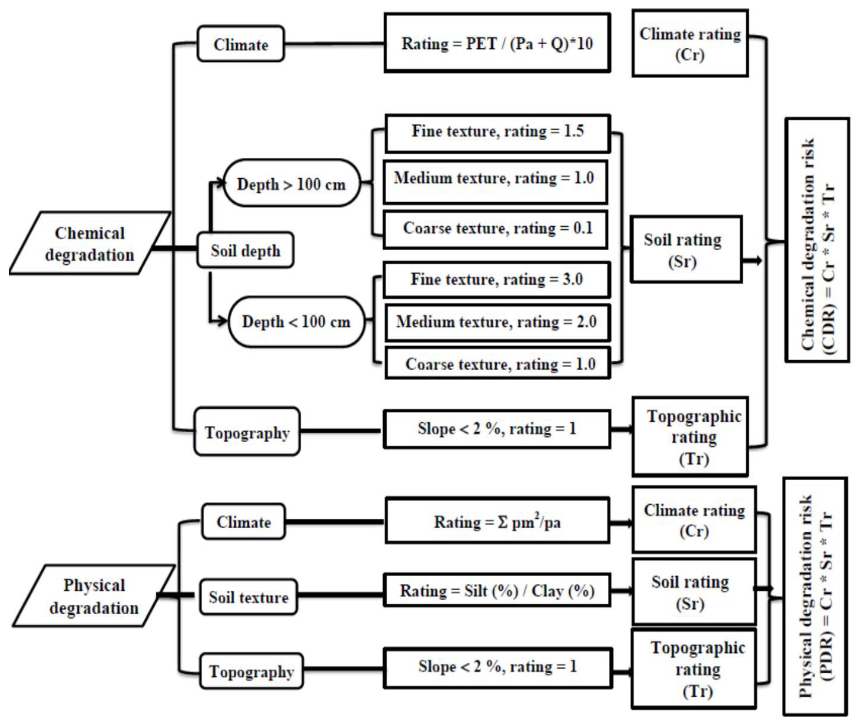
2.4. Soil Degradation Assessment

The type and the degree of soil degradation were defined and described using the methodology of [43].

The risk of degradation was evaluated according to the equations shown in Figure 1.

3. Results and Discussion

The data in Table 2 display the physical and chemical characteristics of the investigated soil profiles in relation to the soils of the flood plain and the lacustrine plain.

3.1. Soils of the Flood Plain

This landscape included five landforms, i.e., terraces (high (AT1), moderate (AT2) and low (AT3)), overflow basins (AB2), and decantation basins (AB1).

The analytical results showed that the soil depth was moderately deep to deep. Soil texture varied greatly within the different geomorphological units. It was found that clay texture was dominant for most of the soil profiles, while (AT2) had a clay loam texture. On the other hand, (AT1) was characterized by its loam texture. The soil pH values were relatively less than 8.50, ranging between 8.14 and 8.48. Soil salinity values showed that the EC varied from 0.84 to 5.97 dS/m. Bulk density values ranged from 1.06 to 1.48 g/cm³. The content of calcium carbonate showed that it increased slightly in the surface layers and ranged from 1.39% to 4.77%.

The content of organic matter was generally considered relatively low as a result of the effect of arid conditions effects, ranging from 0.29% to 1.79%, and gradually decreased with depth, while its highest values were recorded in the surface layers as a result of various agricultural practices and activities. The cation exchange capacity varied between the mapping units due to its high correlation with the texture and type of clay minerals. The results indicated that the medium texture had a low CEC between 14.90 and 23.18 cmolc/kg, while the fine texture was found to have a high CEC between 32.28 and 48.48 cmolc/kg. The exchangeable sodium percentage (ESP) ranged from 2.66% to 20.77%, and the same conclusion was reached by [45].

Table 2. The main physical and chemical properties of the studied soil profiles.

Map. Unit	Profile No.	Depth (cm)	PH 01:02.5	EC (dS/m)	CEC (cmolc/kg)	ESP (%)	OM (%)	CaCO3 (%)	Bulk Density (g/cm3)	Particle Size Distribution (%)
										Coarse	Fine	Silt (%)	Clay (%)	Texture
										Sand (%)	Sand (%)
AT1	1	150	8.33	0.84	14.90	2.66	0.29	2.95	1.35	4.55	31.77	41.97	21.7	Loam
AT2	2	150	8.43	0.84	20.68	3.12	0.30	3.30	1.31	7.6	39.45	27.9	25.05	Sandy clay loam
	3	120	8.22	3.13	26.21	13.04	0.29	2.36	1.44	5.32	27.67	33.22	33.77	Clay loam
	4	145	8.22	3.04	22.65	11.30	0.49	2.52	1.45	3.27	21.35	39.95	35.42	Clay loam
AT3	5	138	8.14	3.44	27.12	7.54	0.65	1.56	1.48	2.16	22.43	39.33	36.06	Clay loam
	6	95	8.37	5.81	32.72	18.97	0.76	3.12	1.24	2.65	16.35	38.35	42.6	Clay
	7	117	8.33	2.37	35.97	8.55	0.80	1.39	1.3	1.73	8.1	45.4	44.7	Silty clay
	8	91	8.43	5.42	34.97	14.66	0.77	1.94	1.28	5.2	15.13	36.8	42.8	Clay
	9	150	8.20	2.49	30.61	9.30	0.51	3.58	1.46	3.7	22.62	37.67	36.00	Clay loam
AB2	10	115	8.44	4.88	43.95	11.91	1.30	3.71	1.20	1.65	9.75	37.35	51.25	Clay
	11	110	8.17	3.55	41.45	10.63	0.83	4.77	1.06	4.36	13.03	38.5	44.26	Clay
	12	130	8.19	1.95	46.86	6.60	1.17	1.82	1.32	2.96	12.36	36.7	47.96	Clay
AB1	13	125	8.48	4.13	44.41	13.30	1.51	2.90	1.16	2.6	11.2	32.43	53.76	Clay
	14	120	8.42	3.56	52.03	8.42	0.90	2.52	1.16	3.06	12.03	29.16	55.73	Clay
	15	135	8.31	4.89	45.75	17.90	1.08	3.04	1.39	0.76	5.86	35.36	58.00	Clay
	16	110	8.29	5.97	51.71	20.77	1.79	2.47	1.22	2.6	8.1	30.3	59.00	Clay
LT1	17	150	8.19	3.07	19.93	9.27	0.56	1.91	1.54	5.7	23.82	43.8	26.67	Loam
LT3	18	140	8.26	2.22	23.58	9.05	0.65	3.29	1.50	3.03	27.8	37.56	31.6	Clay loam
LB2	19	120	8.42	4.37	47.51	13.81	2.11	4.17	1.20	7.85	17.00	22.35	52.8	Clay
	20	140	8.31	3.96	46.35	12.83	1.27	6.35	1.33	7.1	15.47	26.5	50.93	Clay
	21	115	8.38	4.81	41.89	12.89	1.50	1.38	1.23	4.85	12.05	25.35	57.75	Clay
LB1	22	85	8.41	8.36	48.96	18.71	1.60	8.02	1.36	4.47	10.3	21.27	63.95	Clay
	23	130	8.23	5.82	55.79	13.27	1.56	6.23	1.33	6.00	15.75	18.82	59.42	Clay
	24	80	8.37	9.20	43.11	22.87	1.36	5.36	1.02	2.32	8.9	21.95	66.82	Clay

Table 2. The main physical and chemical properties of the studied soil profiles.

Map. Unit	Profile No.	Depth (cm)	PH 01:02.5	EC (dS/m)	CEC (cmolc/kg)	ESP (%)	OM (%)	CaCO3 (%)	Bulk Density (g/cm3)	Particle Size Distribution (%)
										Coarse	Fine	Silt (%)	Clay (%)	Texture
										Sand (%)	Sand (%)
AT1	1	150	8.33	0.84	14.90	2.66	0.29	2.95	1.35	4.55	31.77	41.97	21.7	Loam
AT2	2	150	8.43	0.84	20.68	3.12	0.30	3.30	1.31	7.6	39.45	27.9	25.05	Sandy clay loam
	3	120	8.22	3.13	26.21	13.04	0.29	2.36	1.44	5.32	27.67	33.22	33.77	Clay loam
	4	145	8.22	3.04	22.65	11.30	0.49	2.52	1.45	3.27	21.35	39.95	35.42	Clay loam
AT3	5	138	8.14	3.44	27.12	7.54	0.65	1.56	1.48	2.16	22.43	39.33	36.06	Clay loam
	6	95	8.37	5.81	32.72	18.97	0.76	3.12	1.24	2.65	16.35	38.35	42.6	Clay
	7	117	8.33	2.37	35.97	8.55	0.80	1.39	1.3	1.73	8.1	45.4	44.7	Silty clay
	8	91	8.43	5.42	34.97	14.66	0.77	1.94	1.28	5.2	15.13	36.8	42.8	Clay
	9	150	8.20	2.49	30.61	9.30	0.51	3.58	1.46	3.7	22.62	37.67	36.00	Clay loam
AB2	10	115	8.44	4.88	43.95	11.91	1.30	3.71	1.20	1.65	9.75	37.35	51.25	Clay
	11	110	8.17	3.55	41.45	10.63	0.83	4.77	1.06	4.36	13.03	38.5	44.26	Clay
	12	130	8.19	1.95	46.86	6.60	1.17	1.82	1.32	2.96	12.36	36.7	47.96	Clay
AB1	13	125	8.48	4.13	44.41	13.30	1.51	2.90	1.16	2.6	11.2	32.43	53.76	Clay
	14	120	8.42	3.56	52.03	8.42	0.90	2.52	1.16	3.06	12.03	29.16	55.73	Clay
	15	135	8.31	4.89	45.75	17.90	1.08	3.04	1.39	0.76	5.86	35.36	58.00	Clay
	16	110	8.29	5.97	51.71	20.77	1.79	2.47	1.22	2.6	8.1	30.3	59.00	Clay
LT1	17	150	8.19	3.07	19.93	9.27	0.56	1.91	1.54	5.7	23.82	43.8	26.67	Loam
LT3	18	140	8.26	2.22	23.58	9.05	0.65	3.29	1.50	3.03	27.8	37.56	31.6	Clay loam
LB2	19	120	8.42	4.37	47.51	13.81	2.11	4.17	1.20	7.85	17.00	22.35	52.8	Clay
	20	140	8.31	3.96	46.35	12.83	1.27	6.35	1.33	7.1	15.47	26.5	50.93	Clay
	21	115	8.38	4.81	41.89	12.89	1.50	1.38	1.23	4.85	12.05	25.35	57.75	Clay
LB1	22	85	8.41	8.36	48.96	18.71	1.60	8.02	1.36	4.47	10.3	21.27	63.95	Clay
	23	130	8.23	5.82	55.79	13.27	1.56	6.23	1.33	6.00	15.75	18.82	59.42	Clay
	24	80	8.37	9.20	43.11	22.87	1.36	5.36	1.02	2.32	8.9	21.95	66.82	Clay

Soils of the Lacustrine Plain

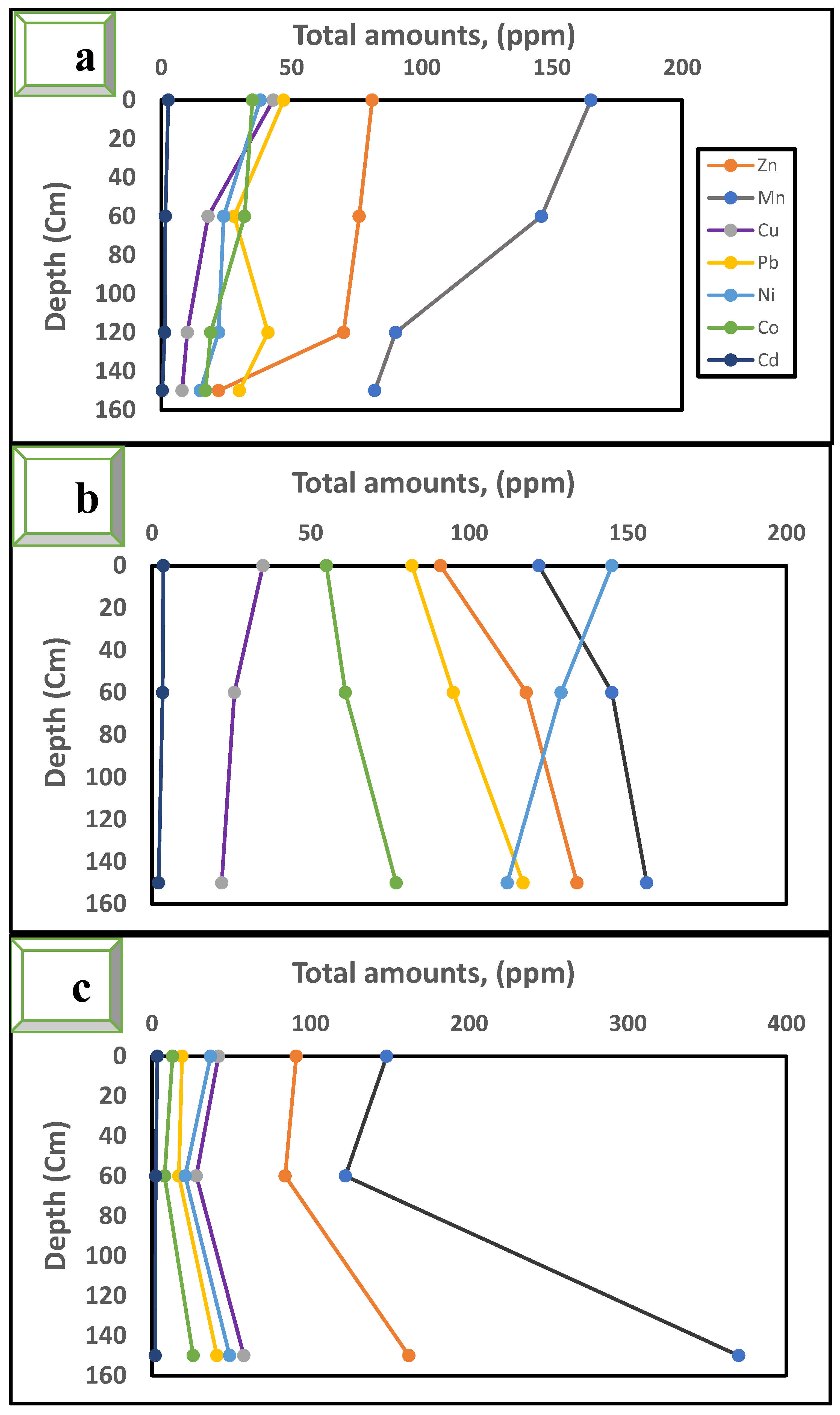
This landscape included four landforms, i.e., terraces (high (LT1) and low (LT3)), overflow basins (LB2), and decantation basins (LB1).

The analytical data indicated that the soil depth was moderately shallow to deep. On the other hand, it was observed in the field examination that gleying and mottling was present in the deep layers of some soil profiles as a result of the influence of the water table level fluctuation in this zone [46]. A great variety of soil texture in this landscape was identified, from loam to clay. The soil pH values ranged from 8.19 to 8.42. The EC values varied widely, ranging from 2.22 to 9.20 dS/m. The bulk density value varied from 1.02 to 1.54 g/cm³. The CaCO₃ varied between 1.38% and 8.02%, and its height was observed in the deeper layers due to its association with the presence of shell fragments, that is richness with a carbonate component derived from a terrestrial origin [47].

The content of organic matter in this landscape was relatively high, ranging from 0.56% to 2.11%, and its distribution appeared to show irregular behavior where the organic matter content decreased in the subsurface layers and then increased in the deeper layers. This can be explained by the high OM content in saline soils which may be due to its preservation by the salts. Furthermore, the high content of OM in the deepest layers may be due to dissolution of humus as sodium humate and its movement down in the profile. Moreover, the increase in clay fraction encourages the formation of clay humus complex which is more resistant to decomposition than organic matter alone [48]. The CEC values varied widely due to the types of heavy texture and their contents which varied between 19.93 and 49.29 cmolc/kg. The ESP values ranged from 9.05% to 22.87%.

3.2. Heavy Metals

The results (

Table 3. Maximum (max), minimum (min), and mean values of total heavy metals (ppm).

	Fe	Mn	Zn	Cu	Pb	Ni	Co	Cd
Max	67,359.3	1394.72	310.15	86.14	168.51	145.32	87.26	5.43
Min	2871.5	74.51	11.21	7.98	7.31	4.88	7.87	0.20
Mean	34,621.7	569.93	122.66	44.02	63.12	61.45	32.87	1.98

) indicated that the mean concentrations of heavy metals, i.e., Fe, Mn, Zn, Cu, Pb, Ni, Co, and Cd, in the different geomorphological units were 34,621.7, 569.93, 122.66, 44.02, 63.12, 61.45, 32.87, and 1.98 ppm, respectively. The total of the elements in the different studied profiles were distributed in descending order as follows: Fe > Mn > Zn > Pb > Ni > Cu > Co > Cd.

The results of the vertical distribution in some soil profiles in the different geomorphological units (AT1, AT2, AT3, LT1, and LT3) are shown in Figure 2a. They showed that the contents of all the heavy metals decreased with depth, except for Pb, and that their concentrations increased in the surface layers due to their association with clay and organic matter [49]. Furthermore, they decreased in deep layers due to the dominance of the sand fraction and low CEC [50]. Moreover, it was observed that the silt fraction dominated in these units, causing Pb to present an irregular trend. The presence of reactive elements, such as sesquioxides, in the silt fraction might account for the binding of Pb in this fraction [51].

Regarding the vertical distribution in the mapping units LB2 and LB1, as shown in Figure 2b, the total heavy metals in the studied area increased with the depth, which may be attributed to the increase of the fine fractions. On the other hand, copper (Cu) and nickel (Ni) decreased with the depth and their amounts increased in the surface layer as a result of their bonding with the accumulated organic matter [52].

The results in Figure 2c in the geomorphological units, AB2 and AB1 showed that the tested heavy metals were relatively remarkably low in the subsurface layers and their amounts were high in the surface and deep layers. This can be explained by the fact that high concentrations of heavy metals and their retention in the clay fraction in the deep layers is due to a lack of humus, which determines the migration of free ions to this depth. Moreover, higher concentrations in the surface layers could be due to the presence of high humus contents. The same interpretations were reported by [53,54].

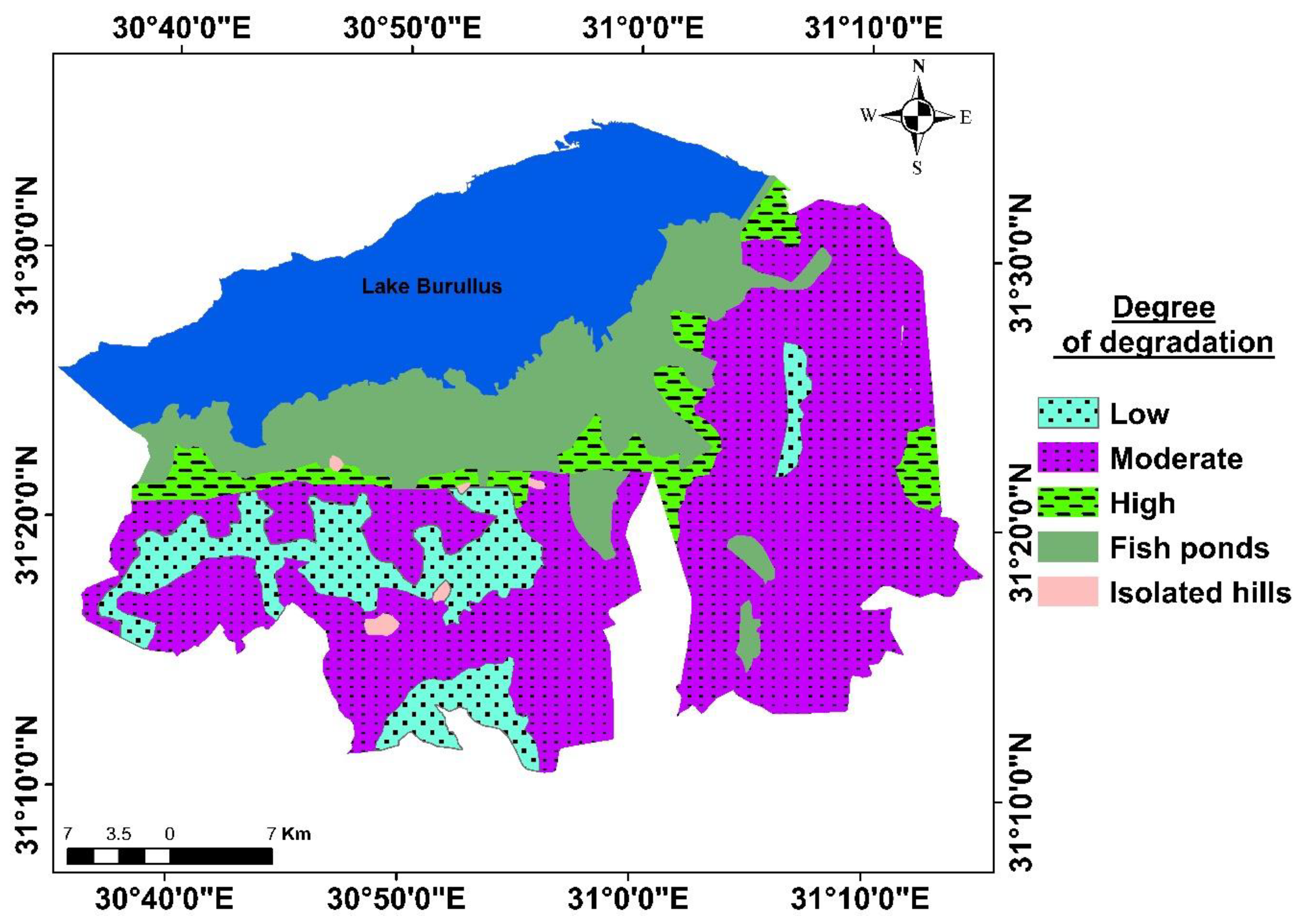
3.3. Soil Degradation

The data in

Table 4. Soil degradation degrees in the different mapping units.

Map. Unit	Chemical Degradation				Physical Degradation
	Salinization		Alkalization		Compaction		Water Logging
	EC dS/m	Class	ESP (%)	Class	BD (g/cm3)	Class	W.T cm	Class
AT1	0.89	1	2.55	1	1.36	2	150	1
AT2	2.38	1	9.14	1	1.4	3	138	1
AT3	4.5	2	13.11	2	1.36	2	118	2
AB2	3.69	1	9.97	1	1.19	1	118	1
AB1	4.72	2	15.24	3	1.22	2	122	3
LT1	3.54	1	10.27	2	1.55	3	150	2
LT3	2.62	1	10.39	2	1.51	3	140	2
LB2	4.79	2	12.54	2	1.27	2	125	2
LB1	7.87	2	18.64	3	1.23	2	98	3

1 = Low, 2 = Moderate, 3 = High. BD, bulk density.

indicated that the soils of the terraces, AT1, AT2, LT1, and LT3, had a low degree of salinization (EC reached to 0.89 dS/m), as they were characterized by good physical properties. The texture of their deep layers was sandy clay loam, and due to the improved drainage conditions, the ground water level reached 150 cm, which is reflected in the leaching of salts and reduction in their concentration at increasing depths [55]. On the other hand, it was noted that the soil of the over-flow basins (AB2) had low salinity despite its clay texture, and this was confirmed by the field examination of this soil that showed it had a tile drainage system that contributed to a reduction in salt concentrations [56].

In contrast, the salinity incrementally increased in the soils of the decantation basins, AB1 and LB1, especially the soils of lacustrine deposits origin, which had heavy clay content in the deep layers, poor drainage, high ground water, and gleying. All these conditions led to the movement of salts by capillary rise to the surface layers and thus accumulated in them, which is consistence with Reference [57]. The high degree of alkalinization (the ESP reached 18.64%) affected the soil of the decantation basins (AB1 and LB1).

The high degree of compaction affected the values of bulk density (which reached 1.55 g/cm³) in the soil of the terraces (AT2, LT1, and LT3). It was observed that the deeper layers of these soils increased in compaction due to a high sand fraction and low organic matter [58]. Moreover, high compaction was found in the surface layers in the decantation basins soils. This can be explained by the fact that wet-tillage (puddling) caused these layers to be compacted, which reduced the leaching of soluble ions and caused salts to accumulate in them. The migration of clay was also caused by the destruction of the surface structure and changes in its condition from oxidation and reduction, especially in the deposits of lacustrine in the study area. The same analysis was carried out by another researcher who came to the same conclusion [59].

The high degree of water logging (soil depth less than 100 cm) affected the soil of the decantation basins (LB1). This soil was affected by the lacustrine deposits system near Lake Burullus.

The field inspection revealed that excessive irrigation, the use of low-quality water for irrigation, improper use of heavy equipment, human intervention in natural drainage, and a lack of conservation measures were the primary causes of soil deterioration in the studied area.

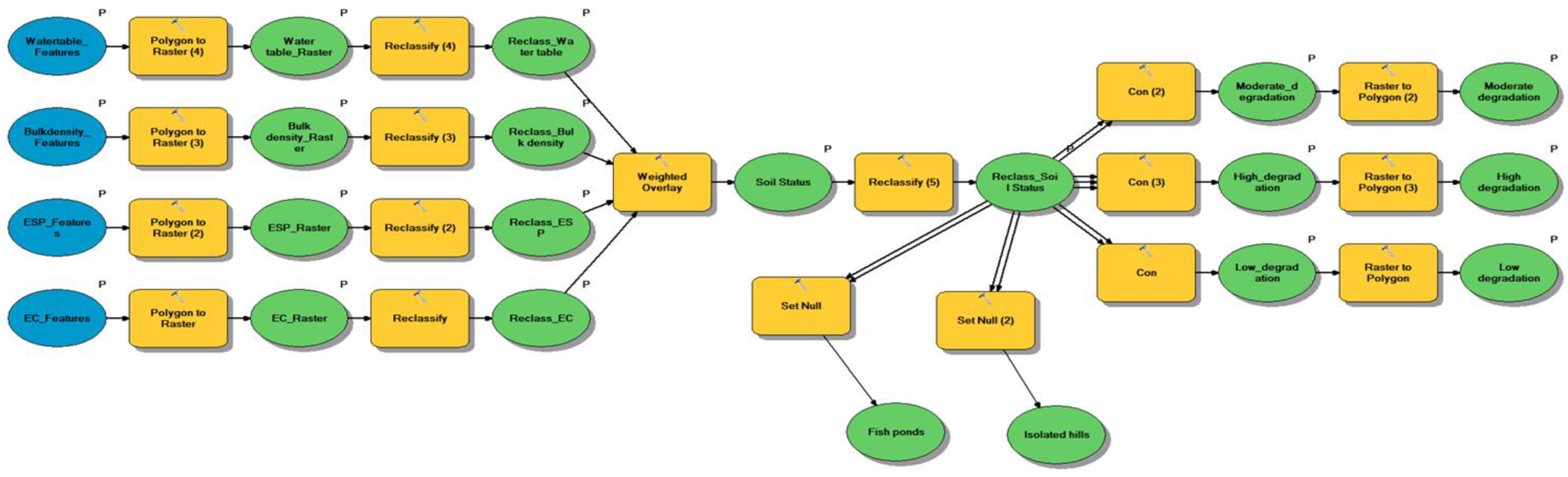
3.3.1. Spatial Soil Degradation Model

A soil degradation spatial model was designed using geoprocessing tools to assess the degree of degradation in the study area (Figure 3). This was carried out with input variables such as salinity, alkalinity, compaction, and water logging to produce a soil degradation map. The model can be thought of as a visual programming language for building workflow, and it comprises a series of sequential steps: (1) converting bulk density, electrical conductivity, exchangeable sodium percentage, and water table depth from vector characteristics into raster layers; (2) reclassifying the variables to the common scale; (3) applying a weighted overlay for the raster layers that were classed by assigning a new value based on an assessment scale to each value class in an input raster and weighting each input raster according to its significance or percent effect. The percent of weight is relative, and the total percent influence weights must be equal 100; (4) reclassifying weighted overlay raster layers; (5) using conditional tools such as setting null to exclude fish ponds and isolated hills from the analysis and also using the con tool to specify only layers that will be used in the study area; (6) converting the raster dataset to polygon features; and (7) producing a soil degradation map.

The results of the spatial model indicated three degrees of degradation in the study area (Figure 4). First, a low degree covering an area of 174.05 km², i.e., 16.61%, was presented in the soils, AT1 and AB2. Second, a moderate degree covering an area of 775.32 km², i.e., 74.03%, was presented in the soils, AT2, AT3, AB1, LT1, LT3, and LB2. Third, a high degree covering an area of 98.11 km², i.e., 9.36%, was presented in the soil LB1.

3.3.2. Soil Degradation Risk Assessment

The dangers associated with soil degradation imply a progressive loss in agricultural production brought on by the combined effects of soil, topography, and climate conditions without human intervention.

The calculated results from the risk equations in

Table 5. The computed chemical and physical degradation risks in the studied area.

Map. Unit	Chemical Degradation Risk					Physical Degradation Risk
	SR	TR	CR	Risk	Class	SR	TR	CR	Risk	Class
AT1	1	1	0.76	0.76	1	1.93	1	4.60	8.87	4
AT2	1	1	0.76	0.76	1	1.07	1	4.60	4.92	3
AT3	1.9	1	1.03	1.95	1	0.97	1	4.60	4.46	3
AB2	1.5	1	0.66	0.99	1	0.78	1	4.60	3.58	2
AB1	1.5	1	0.87	1.30	1	0.55	1	4.60	2.53	2
LT1	1	1	1.51	1.51	1	1.64	1	4.60	7.54	4
LT3	1	1	0.76	0.76	1	1.18	1	4.60	5.42	3
LB2	1.5	1	1.01	1.51	1	0.45	1	4.60	2.07	2
LB1	2.5	1	2.02	5.05	3	0.32	1	4.60	1.47	1

SR, soil rating; TR, topographic rating; CR, climatic rating; Risk = SR*TR*CR; risk < 2 (class 1 = low), risk = 2–4 (class 2 = moderate), risk = 4–6 (class 3 = high), risk > 6 (class 4 = very high).

revealed that the geomorphological units, LB1, LB2, AB1, and AB2, had physical degradation ranging from low to moderate risks, as they covered an area of 98.22 km², i.e., 9.37%, and 435.11 km², i.e., 41.53%, respectively. The reduced risk of physical degradation of these units was due to the fact that they were characterized by a decrease in silt fraction and an increase in the content of organic matter. However, the units, AT2, AT3, LT3, AT1, and LT1, had physical degradation ranging from high to very high risks, covering an area of 420.52 km², i.e., 40.14%, and 93.63 km², i.e., 8.93%, respectively. This rise was associated with an increase in the silt fraction and a decrease in the content of organic matter. These trends were similar to [60].

The results in Table 5 revealed that the mapping units, AT1, AT2, AT3, AB2, AB1, LT1, LT3, and LB2, were characterized by having a low risk of chemical degradation as a result of their soil depths exceeding 100 cm and the vast majority of their units covered an area of 949.26 km², i.e., 90.62%. Moreover, one unit (LB1) was found to have a high risk of chemical degradation. This may be explained by its depths being less than 100 cm, as well as the high salinity of the ground water, and it covering a small area, 98.22 km², i.e., 9.37%.

3.4. Pollution Indices

3.4.1. Enrichment Factor (EF)

The enrichment factor (EF) gives reliable information in geochemical studies, as it is used to distinguish sources of heavy metal enrichment originating from either natural geological processes or anthropogenic factors [61].

The EF was calculated from the equation provided by [62,63].

Enrichment Factor (EF) = (M/Fe) sample/(M/Fe) background

where (M/Fe) is the ratio of metal and Fe concentrations of the sample, M/Fe crust is the ratio of metal and Fe concentrations of the background, and M is the concentration of metal. In the current study, the background concentrations of the eight metals were taken from [64].

The classes of EF were as follows:

EF ≤ 1 (no enrichment), 1 < EF ≤ 3 (minor enrichment), 3 < EF ≤ 5 (moderate enrichment), 5 < EF ≤ 10 (moderately severe enrichment), 10 < EF ≤ 25 (severe enrichment), 25 < FE ≤ 50 (very severe enrichment), and EF > 50 (extremely severe enrichment) [65].

The calculated results for the enrichment factor (EF) of the heavy metals as shown in

Table 6. Enrichment factor (EF) values of the investigated heavy metals.

Map. Unit	Mn	Zn	Cu	Pb	Ni	Co	Cd
AT1	2.37	2.64	4.41	15.59	1.41	10.10	22.31
AT2	0.78	1.70	2.05	4.09	1.00	2.62	10.80
AT3	1.01	2.03	2.14	4.78	1.26	2.87	11.83
AB2	0.69	1.79	1.13	3.10	1.08	2.45	11.54
AB1	0.93	1.87	1.17	3.52	1.50	2.29	7.88
LT1	2.41	1.47	3.93	14.71	2.03	5.96	26.99
LT3	0.45	1.84	2.05	1.66	1.99	3.57	12.41
LB2	0.70	1.38	1.07	4.77	1.25	1.29	7.98
LB1	1.04	2.04	1.22	5.05	1.18	2.47	8.92

indicated that the degree of enrichment varied among the different geomorphological units, as there was no enrichment to minor enrichment with Mn and Ni, minor enrichment with Zn, minor enrichment to moderate enrichment with Cu, minor enrichment to severe enrichment with Pb and Co, and moderately severe enrichment to very severe enrichment with Cd. The EF sequences of heavy metals in the different geomorphological units were represented in the following order: Cd > Pb > Co > Cu > Zn > Mn > Ni. Thus, it was concluded that cadmium was more abundant in its enrichment than other metals and that its higher enrichment was due to human activities from excessive uses of superphosphate fertilizer applications by farmers; the same interpretation was reported by [66]. In contrast, the EF values for some metals were the lowest as a result of the higher total amounts of iron.

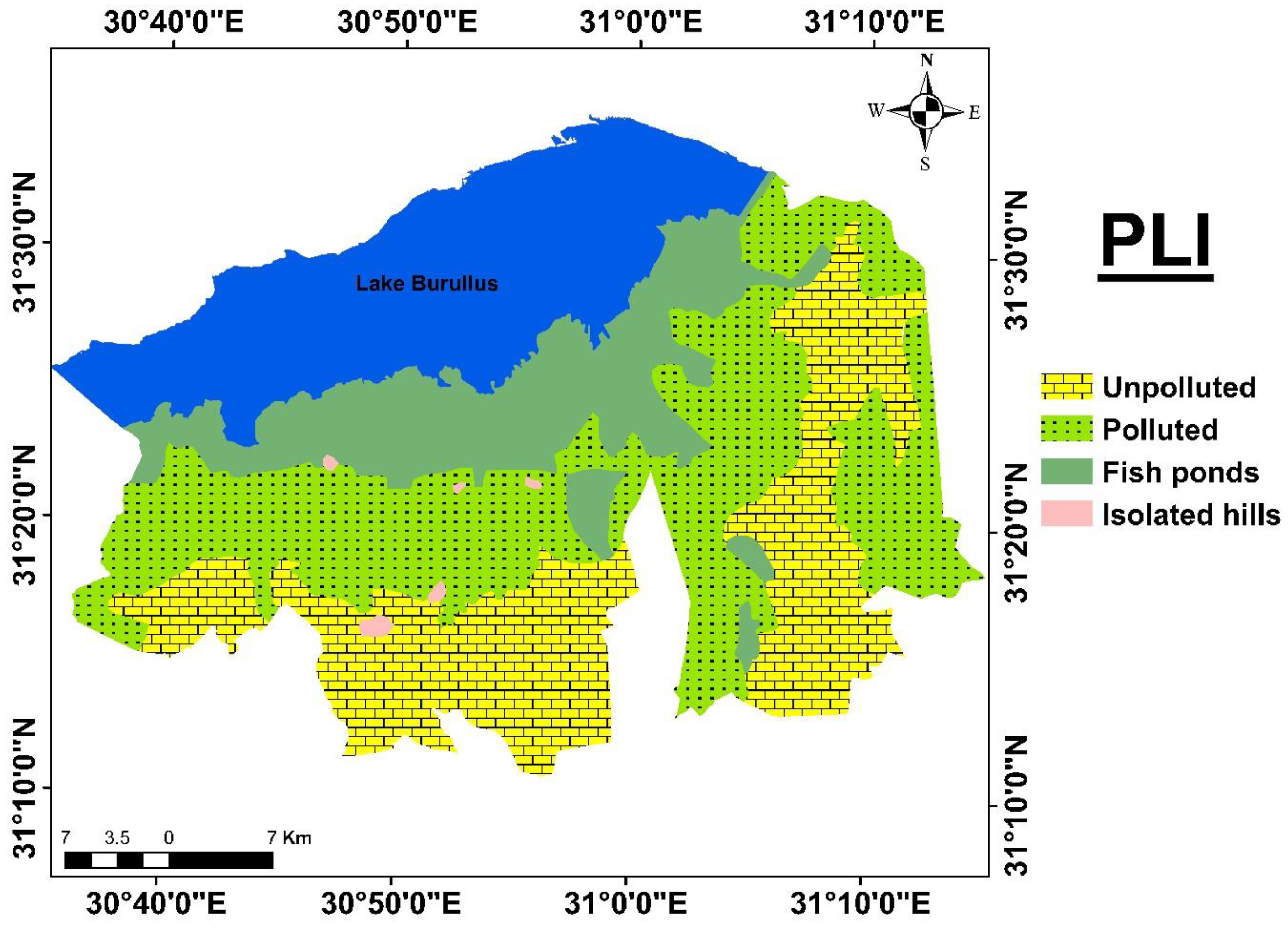
3.4.2. Pollution Load Index (PLI)

The pollution load index (PLI) expresses the number of times the concentration of heavy metals in the samples exceeds the background concentration and gives an overall assessment of heavy metal toxicity in the study area [67].

The pollution load index (PLI) of each site was evaluated as indicated by [67].

Pollution load index = (CF1 × CF2 × ………CFn)^1/n

where n is the number of metals and CF is the contamination factor. Contamination can be estimated as: PLI >1 means polluted; PLI value < 1 means unpolluted, according to [68,69].

The pollution load indices (PLI) calculated from the values of the contamination factor (CF) of the heavy metals presented in

Table 7. Values of pollution load indices (PLI) and potential ecological risk indices (PER) for the measured heavy metals in the studied area.

Map. Unit	PLI		PER
	Value	Level	Value	Level
AT1	0.48	Unpolluted	95.28	Low risk
AT2	0.77	Unpolluted	153.62	Moderate risk
AT3	0.88	Unpolluted	149.02	Low risk
AB2	1.22	Polluted	239.66	Moderate risk
AB1	1.59	Polluted	239.80	Moderate risk
LT1	1.11	Polluted	275.43	Moderate risk
LT3	0.83	Unpolluted	194.34	Moderate risk
LB2	1.69	Polluted	316.46	Considerable risk
LB1	2.63	Polluted	414.65	Considerable risk

showed that the majority of the studied profiles were polluted (PLI > 1) while some profiles were unpolluted (PLI < 1).

The spatial distribution of the PLI (Figure 5) showed that the sites with a high level of pollution, with an area of 589.4 km², i.e., 56.26%, comprised the mapping units AB2, AB1, LT1, LB2, and LB1, while the unpolluted sites with an area of 458.8 km², i.e., 43.73%, comprised the mapping units AT1, AT2, AT3, and LT3.

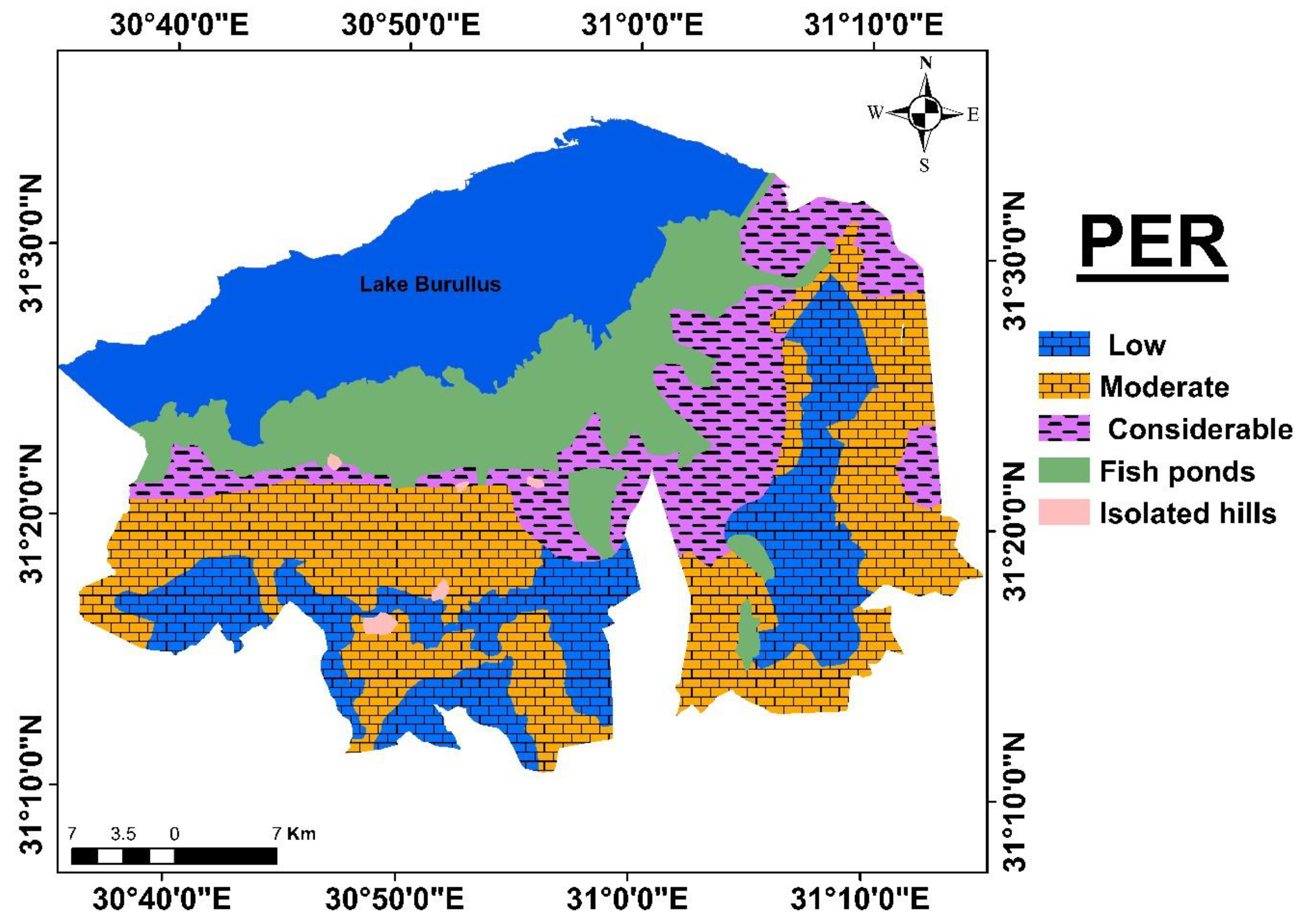
3.4.3. Potential Ecological Risk Index (PER)

The potential ecological risk index (PER) can be used to make a comprehensive assessment of the ecological risks caused by toxic metals.

The PER was calculated using the following equation:

PER = ∑ Er

where Er was the potential ecological risk factor of each heavy metal.

The following classes of the PER were in accordance with [70], where PER < 150 (low), 150 < PER < 300 (moderate), 300 < PER < 600 (considerable), and PER > 600 (very high).

The obtained results (Table 7) indicated that the PER values in most geomorphological units indicated the moderate risk, and the PER values indicated the high risk in other units due to the presence of a high ecological risk of cadmium, which had a high toxicity coefficient. The same interpretation was reported by [70].

As shown in Figure 6, the considerable risk with an area of 249.9 km², i.e., 23.86%, was presented in the geomorphological units LB2 and LB1, the moderate risk with an area of 492.4 km², i.e., 47.01%, was presented in units AT2, AB2, AB1, LT1, and LT3, and the low risk with an area of 305.5 km², i.e., 29.12%, was presented in units AT1 and AT3.

4. Conclusions

It can be concluded that the studied area was subjected a low to high risk of chemical degradation, as well as low to very high risk of physical degradation. Moreover, the processes of salinity, alkalinity, soil compaction, and water logging were from low to high. The GIS is an effective tool to store, manipulate and quantitatively evaluate soil degradation. As a result of the use of waste-water in irrigation, the concentrations of heavy metals were increased in the majority of the study area, and they increased significantly in the basin soils. The pollution load index (PLI) showed that 43.73% of the study area was unpolluted, and 56.26% was polluted. The current status of the study area indicated that it is at high risk of degradation and contamination with heavy metals and thus requires planning and soil management to achieve sustainable agriculture.

References

1. Aksoy, E.; Ozsoy, G.; Dirim, S.M. Soil mapping approach in GIS using Landsat satellite imagery and DEM data. Afr. J. Agric. Res. 2009, 4, 1295–1302. [Google Scholar]
2. FAO. Soil is a non-renewable resource. In 2015 International Year of Soils; Food and Agriculture Organization: Rome, Italy, 2015; Available online: http://www.fao.org/3/a-i4373e.pdf (accessed on 1 July 2021).
3. Shokr, M.S.; Abdellatif, M.A.; El Baroudy, A.A.; Elnashar, A.; Ali, E.F.; Belal, A.A.; Attia, W.; Ahmed, M.; Aldosari, A.A.; Szantoi, Z.; et al. Development of a spatial model for soil quality assessment under arid and semi-arid conditions. Sustainability 2021, 13, 2893. [Google Scholar] [CrossRef]
4. Warren, A.; Agnew, C. An Assessment of Desertification and Land Degradation in Arid and Semi Arid Areas; Paper No. 2; International Institute for Environment and Development: London, UK, 1988. [Google Scholar]
5. Lal, R.; Stewart, B.A. Advances in Soil Science, Soil Degradation; Springer: New York, NY, USA, 1990; p. 349. [Google Scholar]
6. Wim, G.; El-Hadji, M. Causes, General Extent and Physical Consequence of Land Degradation in Arid, Semi Arid and Dry Subhumid Areas; Forest Conservation and Natural Resources, Forest Department; FAO: Rome, Italy, 2002. [Google Scholar]
7. Liberti, M.; Simoniello, T.; Carone, M.T.; Coppola, R.; Emilio, M.D.; Macchiato, M. Mapping badland areas using LANDSAT TM/ETM satellite imagery and morphological data. Geomorphology 2009, 106, 333–343. [Google Scholar] [CrossRef]
8. Gomiero, T. Soil Degradation, Land Scarcity and Food Security:Reviewing a Complex Challenge. Sustainability 2016, 8, 281. [Google Scholar] [CrossRef] [Green Version]
9. Bridges, E.M.; Oldeman, L.R. Global assessment of human-induced soil degradation. Arid Soil Res. Rehabil. 1999, 13, 319–325. [Google Scholar] [CrossRef]
10. Ali, R.; Abdel-Kawy, W.A. Land degradation risk assessment of El Fayoum depression, Egypt. Arab. J. Geosci. 2013, 6, 2767–2776. [Google Scholar] [CrossRef]
11. UNCCD. United Nations Convention to Combat Desertification in Those Countries Experiencing Serious Drought and/or Desertification, Particularly in Africa; UNCCD: Paris, France, 1994. [Google Scholar]
12. Lal, R. Soil degradation by erosion. Land Degrad. Dev. 2001, 12, 519–539. [Google Scholar] [CrossRef]
13. Lal, R. Restoring Soil Quality to Mitigate Soil Degradation. Sustainability 2015, 7, 5875–5895. [Google Scholar] [CrossRef] [Green Version]
14. Lal, R. Soils and sustainable agriculture, a review. Agron. Sustain. Dev. 2008, 28, 57–64. [Google Scholar] [CrossRef]
15. Uchida, S. Applicability of satellite remote sensing for mapping hazardous state of land degradation by soil erosion on agricultural areas. Procedia Environ. Sci. 2015, 24, 29–34. [Google Scholar] [CrossRef] [Green Version]
16. Dwivedi, R.S.; Sreenivas, K.; Ramana, K.V. Inventory of salt affected soils and water-logged areas: A remote sensing approach. Int. J. Remote Sens. 1999, 20, 1589–1599. [Google Scholar] [CrossRef]
17. Darwish, K.H.; Abdel Kawy, W.A. Quantitive Assessment of Soil Degradation in some Areas North Nile Delta, Egypt. Int. J. Geol. 2008, 2, 17–22. [Google Scholar]
18. Wahab, M.A.; Rasheed, M.A.; Youssef, R.A. Degradation hazard assessment of some soils north Nile Delta, Egypt. J. Am. Sci. 2010, 6, 156–161. [Google Scholar]
19. Abdel Kawy, W.A.; Ali, R.R. Assessment of soil degradation and resilience at northeast Nile Delta, Egypt: The impact on soil productivity. Egypt. J. Remote Sens. Space Sci. 2012, 15, 19–30. [Google Scholar] [CrossRef] [Green Version]
20. Shalaby, A.; Ali, R.; Gad, A. Land Degradation Monitoring in the Nile Delta of Egypt, using Remote Sensing and GIS. Int. J. Basic Appl. Sci. 2012, 1, 292–303. [Google Scholar]
21. Hamed, Y.; Salem, S.h.; Ali, A.; Sheshtawi, A. Environmental Effect of Using Polluted Water in New/Old Fish Farms. Recent Advances in Fish Farms In Tech. 2011. Available online: http://cdn.intechopen.com/pdfs-wm/24077.pdf (accessed on 10 November 2014).
22. Liu, W.H.; Zhao, J.Z.; Ouyang, Z.Y.; Söderlund, L.; Liu, G.H. Impacts of sewage irrigation on heavy metal distribution and contamination in Beijing, China. Environ. Int. 2005, 31, 805–812. [Google Scholar] [CrossRef]
23. Ai, P.; Jin, K.; Alengebawy, A.; Elsayed, M.; Meng, L.; Chen, M.; Ran, Y. Effect of application of different biogas fertilizer on eggplant production: Analysis of fertilizer value and risk assessment. Environ. Technol. 2020, 19, 101019. [Google Scholar] [CrossRef]
24. Mbah, C.; Anikwe, M. Variation in heavy metal contents on roadside soils along a major expressway in south east Nigeria. N. Y. Sci. J. 2010, 3, 103–107. [Google Scholar]
25. Sofianska, E.; Michailidis, K.; Mladenova, V.; Filippidis, A. Multivariate Statistical and GIS-Based Approach to Identify Heavy Metal Sources in Soils of the Drama Plain, Northern Greece. National Conference with International Participation, Geosci. 2013, pp. 131–132. Available online: https://www.bgd.bg/CONFERENCES/Geonauki_2013/Sbornik/pdf/55_Sofianska_GeoSci_2013.pdf (accessed on 1 July 2021).
26. Farmer, J.G. The perturbation of historical pollution records in aquatic sediments. Environ. Geochem. Health 1991, 13, 76–83. [Google Scholar] [CrossRef]
27. He, H.; Shi, L.; Yang, G.; You, M.; Vasseur, L. Ecological Risk Assessment of Soil Heavy Metals and Pesticide Residues in Tea Plantations. Agriculture 2020, 10, 47. [Google Scholar] [CrossRef] [Green Version]
28. Abowaly, M.E.; Belal, A.-A.A.; Abd Elkhalek, E.E.; Elsayed, S.; Abou Samra, R.M.; Alshammari, A.S.; Moghanm, F.S.; Shaltout, K.H.; Alamri, S.A.M.; Eid, E.M. Assessment of Soil Pollution Levels in North Nile Delta, by Integrating Contamination Indices, GIS, and Multivariate Modeling. Sustainability 2021, 13, 8027. [Google Scholar] [CrossRef]
29. El-Amier, Y.A.; Bessa, A.Z.E.; Elsayed, A.; El-Esawi, M.A.; AL-Harbi, M.S.; Samra, B.N.; Kotb, W.K. Assessment of the Heavy Metals Pollution and Ecological Risk in Sediments of Mediterranean Sea Drain Estuaries in Egypt and Phytoremediation Potential of Two Emergent Plants. Sustainability 2021, 13, 12244. [Google Scholar] [CrossRef]
30. Sun, B.; Li, Z.; Gao, Z.; Guo, Z.; Wang, B.; Hu, X.; Bai, L. Grassland degradation and restoration monitoring and driving forces analysis based on long time-series remote sensing data in XilinGol league. Acta Ecol. Sin. 2017, 37, 219–228. [Google Scholar] [CrossRef]
31. Egyptian Meteorological Authority. Climatic Atlas of Egypt; Arab Republic of Egypt, Ministry of Transport: Cairo, Egypt, 2016. [Google Scholar]
32. Soil Survey Staff. Keys to Soil Taxonomy; Department of Agriculture, Natural Resources Conservation Service: Washington, WA, USA, 2014. [Google Scholar]
33. Shata, A.A.; Fayoumy, E.I. Remarks on the regional geological structure of the Nile Delta. In Proceedings of the Bucharest Symposium for Hydrology of the Delta, Bucharest, Romania, 6–9 May 1969. [Google Scholar]
34. Abou El Enain, A.S. Use G.I.S. Remote Sensing and Aerial Photo-Interpretation Techniques for Mapping and Evaluating Soil Improvement in Some Areas of North Nile Delta, Egypt. Ph.D. Thesis, Faculty of Agriculture, Cairo University, Cairo, Egypt, 1997. [Google Scholar]
35. ITT. ITT Corporation ENVI 5.1 Software, ITT: White Plains, NY, USA, 2009.
36. Lillesand, T.M.; Kiefer, R.W. Remote Sensing and Image Interpretation; John Wiley: New York, NY, USA, 2007. [Google Scholar]
37. Zinck, J.A.; Valenzuela, C.R. Soil geographic database structure and application examples. ITC J. 1990, 3, 270–294. [Google Scholar]
38. Dobos, E.; Norman, B.; Bruee, W.; Luca, M.; Chris, J.; Erika, M. The Use of DEM and Satellite Images for Regional Scale Soil Database. In Proceedings of the 17th World Congress of Soil Science (WCSS), Bangkok, Thailand, 14–21 August 2002. [Google Scholar]
39. FAO. Guidelines for Soil Description, 4th ed.; FAO: Rome, Italy, 2006. [Google Scholar]
40. Klute, A. (Ed.) Methods of Soil Analysis (Part 1) Physical and Mineralogical Methods; American Society of Agronomy and Soil Science Society of America: Madison, WI, USA, 1986. [Google Scholar]
41. Burt, R. Soil Survey Laboratory Methods Manual, Soil Survey Investigation; Report No. 42 Version 4.0; USDA: Washington, WA, USA, 2004. [Google Scholar]
42. Cottenie, A.; Verloo, M.; Velghe, G.; Kiekens, L. Biological and Analytical Aspects of Soil Pollution; Laboratory of Analytical Agrochemistry, State University: Gent, Belgium, 1982. [Google Scholar]
43. FAO/UNEP. A Provisional Methodology for Soil Degradation Assessment; FAO: Rome, Italy, 1979; p. 48. [Google Scholar]
44. Abuzaid, A.S. Assessing degradation of floodplain soils in north east Nile Delta, Egypt. Egypt. J. Soil Sci. 2018, 58, 135–146. [Google Scholar] [CrossRef] [Green Version]
45. Kome, G.K.; Enang, R.K.; Tabi, F.O.; Yerima, B.P.K. Influence of clay minerals on some soil fertility attributes: A review. Open J. Soil Sci. 2019, 9, 155–188. [Google Scholar] [CrossRef]
46. Bedard-Haughn, A. Gleysolic soils of Canada: Genesis, distribution, and classification. Can. J. Soil Sci. 2011, 91, 763–779. [Google Scholar] [CrossRef]
47. Draz, S.E.O.; Youssef, D.H.; El-Said, G.F. Sedimentological characteristics and distribution of fluoride in granulometric fractions of subsurface sediments in Suez and Aqaba Gulfs, Egypt. J. Egypt. Acad. Soc. Environ. Dev. D-Environ. Stud. 2009, 10, 73–91. [Google Scholar]
48. Chen, Y.; Stevenson, F.J. The Role of Organic Matter in Modern Agriculture; Chen, Y., Acenmelech, Y., Eds.; Martinus Nijhoff: Dorderecht, The Netherlands, 1986; pp. 73–112. [Google Scholar]
49. Chen, Y.M.; Gao, J.B.; Yuan, Y.Q.; Ma, J.; Yu, S. Relationship between heavy metal contents and clay mineral properties in surface sediments: Implications for metal pollution assessment. Cont. Shelf Res. 2016, 124, 125–133. [Google Scholar] [CrossRef]
50. Krzysztof, F.; Małgorzata, K.; Anna, G.; Agnieszka, P. The influence of selected soil parameters on the mobility of heavy metals in soils. Inżynieria i Ochrona Środowiska 2012, 15, 81–92. [Google Scholar]
51. Sutherland, R.A. Lead in grain size fractions of road deposited sediment. Environ. Pollut. 2003, 121, 229–237. [Google Scholar] [CrossRef]
52. Boiteau, R.M.; Till, C.P.; Ruacho, A.; Bundy, R.M.; Hawco, N.J.; McKenna, A.M.; Repeta, D.J. Structural characterization of natural nickel and copper binding ligands along the US GEOTRACES Eastern Pacific Zonal Transect. Front. Mar. Sci. 2016, 3, 243. [Google Scholar] [CrossRef] [Green Version]
53. Damian, F.; Damian, G.; Radu, L.R.; Macovei, G.; Iepure, G.; Napradean, I.; Chira, R.; Kollar, L.; Rata, L.; Zaharia, D.C. Soils from the Baia Mare Zone and the Heavy Metals Pollution. Carpthian J. Earth Environ. Sci. 2008, 3, 85–98. [Google Scholar]
54. Damian, G.; Iepure, Z.S.G.; Damian, F. Distribution of heavy metals in granulometric fractions and on soil profiles. Carpathian J. Earth Environ. Sci. 2019, 14, 343–351. [Google Scholar] [CrossRef]
55. Pazira, E.; Homaee, M. Salt leaching efficiency of subsurface drainage systems at presence of diffusing saline water table boundary: A case study in Khuzestan plains, Iran. In Proceedings of the 9th International Drainage Symposium Held Jointly with CIGR and CSBE/SCGAB Proceedings, Quebec City, QC, Canada, 13–16 June 2010; American Society of Agricultural and Biological Engineers: St. Joseph, MI, USA, 2010; p. 1. [Google Scholar]
56. Ghafoor, A.; Murtaza, G.; Rehman, M.Z.; Sabir, M. Reclamation and salt leaching efficiency for tile drained saline-sodic soil using marginal quality water for irrigating rice and wheat crops. Land Degrad. Dev. 2012, 23, 1–9. [Google Scholar] [CrossRef]
57. Van Hoorn, J.W. Salt transport in heavy clay soil. In Proceedings of the ISSS Symposium on Water and Solute Movement in Heavy Clay Soils, Wageningen, The Netherlands, 27–31 August 1984; pp. 229–240. [Google Scholar]
58. Xu, Y.; Jimenez, M.A.; Parent, S.É.; Leblanc, M.; Ziadi, N.; Parent, L.E. Compaction of coarse-textured soils: Balance models across mineral and organic compositions. Front. Ecol. Evol. 2017, 5, 83. [Google Scholar] [CrossRef] [Green Version]
59. Huang, B.; Li, Z.; Li, D.; Yuan, Z.; Chen, Z.; Huang, J. Distribution characteristics of heavy metal(loid)s in aggregates of different size fractions along contaminated paddy soil profile. Environ. Sci. Pollut. Res. 2017, 24, 23939–23952. [Google Scholar] [CrossRef]
60. Kawy, W.A.M.; Darwish, K.M. Assessment of land degradation and implications on agricultural land in Qalyubia Governorate, Egypt. Bull. Natl. Res. Cent. 2019, 43, 70. [Google Scholar] [CrossRef]
61. Praveena, S.M.; Aris, A.Z.; Radojevic, M. Heavy metals dynamics and source in intertidal mangrove sediment of Sabah Borneo Island. Environ. Asia 2010, 3, 79–83. [Google Scholar]
62. Rule, J.H. Assessment of trace element geochemistry of Hampton roads harbor and lower Chesapeake Bay sediments area. Geol. Water Sci. 1986, 8, 209–219. [Google Scholar] [CrossRef]
63. Rubio, B.; Nombela, M.A.; Vilas, F. Geochemistry of major and trace elements in sediments of the Ria de Vigo (NW Spain) an assessment of metal pollution. Mar. Pollut. Bull. 2000, 40, 968–980. [Google Scholar] [CrossRef]
64. Turekian, K.K.; Wedepohl, K.H. Distribution of the elements in some major units of the Earth’s crust. Geol. Soc. Am. 1961, 72, 175–192. [Google Scholar] [CrossRef]
65. Birch, G. A scheme for assessing human impacts on coastal aquatic environments using sediments. In Coastal GIS; Woodcoffe, C.D., Furness, R.A., Eds.; Wollongong University Papers in Center for Maritime Policy: Wollongong, Australia, 2003; Volume 14. [Google Scholar]
66. Kelliher, F.M.; Gray, C.W.; Noble, A.D. Superphosphate fertiliser application and cadmium accumulation in a pastoral soil. N. Z. J. Agric. Res. 2017, 60, 404–422. [Google Scholar] [CrossRef]
67. Tomilson, D.C.; Wilson, D.J.; Harris, C.R.; Jeffrey, D.W. Problem in assessment of heavy metals in estuaries and the formation of pollution index. Helgoländer Meeresunters. 1980, 33, 566–575. [Google Scholar]
68. Chakravarty, M.; Patgiri, A.D. Metal pollution assessment in sediments of the Dikrong River, NE India. J. Hum. Ecol. 2009, 27, 63–67. [Google Scholar] [CrossRef]
69. Seshan, B.R.R.; Natesan, U.; Deepthi, K. Geochemical and statistical approach for evaluation of heavy metal pollution in core sediments in southeast coast of India. Int. J. Environ. Sci. Technol. 2010, 7, 291–306. [Google Scholar] [CrossRef] [Green Version]
70. Hakanson, L. An ecological risk assessment index for aquatic contamination control, a sedimentogical approach. Water Res. 1980, 14, 975–1001. [Google Scholar] [CrossRef]
Figure 1. Flowchart showing the potential evapotranspiration (PET, mm per year), annual precipitation (PA, mm), monthly precipitation (PM, mm), and quantity of irrigation water (Q) for the risk of soil degradation (mm year−1), in accordance with [44].
Agriculture 13 00076 g001
Figure 2. Distributions of total heavy metals in the different geomorphological units tested: (a) AT1, AT2, AT3, LT1, and LT3; (b) LB2 and LB1; (c) AB2 and AB1. (ac) are symbols.
Agriculture 13 00076 g002
Figure 3. Flowchart of the designed soil degradation model.
Agriculture 13 00076 g003
Figure 4. Soil degradation degrees of the studied area.
Agriculture 13 00076 g004
Figure 5. Pollution load indices (PLI) in the studied area.
Agriculture 13 00076 g005
Figure 6. Potential ecological risk indices (PER) in the studied area.
Agriculture 13 00076 g006