Microscopic Imaging Spray Diagnostics under High Temperature Conditions: Application to Urea–Water Sprays

Abstract

The quantitative investigation of droplet laden turbulent flows at high temperature conditions is of great importance for numerous applications. In this study, an experiment was set up for investigation of evaporating urea–water sprays, which are relevant for the effective reduction of nitrogen oxide emissions of diesel engines using Selective Catalytic Reduction. A shadowgraphy setup is pushed to its limits in order to detect droplet diameters as small as 4 $\mathsf{\mu }\mathrm{m}$ and droplet velocities up to 250 $\mathrm{m}{\mathrm{s}}^{-1}$. In addition, the operating conditions of the gaseous flow of up to 873 $\mathrm{K}$ and $0.6$ $\mathrm{M}$$\mathrm{Pa}$ are an additional challenge. Due to the high temperature environment, image quality is prone to be compromised by Schlieren effects and astigmatism phenomena. A water-cooled window and an astigmatism correction device are installed in order to correct these problems. The results to be presented include characteristics of the turbulent gas flow as well as detailed spray characteristics at different positions downstream of the atomiser. It is demonstrated that the velocity of the gas can be approximated by the velocity of the smallest detectable droplets with sufficient accuracy. Furthermore, the statistical analysis of velocity fluctuations provides data for predicting the turbulent dispersion of the droplets.

1. Introduction

The characterization of sprays is of great importance for many technical applications. Prominent examples are fuel sprays in automotive and aircraft engines or spray drying in industrial processes. The knowledge of droplet size or evaporation rates are essential for the operation of such systems [1]. In this context, spray modelling and numerical predictions are important tools for the design process. The goal of numerous experimental investigations is the tuning of model parameters of semi-empirical submodels or validating submodels and overall simulations [2]. In conclusion, an effective comparison of spray measurements and numerical simulations is the key for a deeper understanding of sprays.

Essential processes like atomisation, spray structure, penetration and evaporation may be affected significantly by temperature, pressure and flow velocity of the ambient gas. Hence, to perform the experimental investigations under typical operating conditions is of major importance. Since in most applications not only the droplet size but also the droplet velocity is of interest, an adequate and established measurement technique is the Phase Doppler Anemometry (PDA). A drawback of this technique is that beam steering may compromise measurements at high temperature conditions [2], which may limit the achievable accuracy or impede the task to obtain quantitative data completely. Nevertheless, successful measurements at technical relevant conditions were published [3].

An alternative to interferometric techniques are imaging diagnostics. In this context, the light sheet configuration in combination with structured illumination has become a prominent technique for the analysis of spray systems in recent years [4,5]. A specific advantage of this configuration is the well-defined measurement volume due to a low contribution of out-of-focus light. However, the line-of-sight arrangement, with camera and illumination on the same optical axis, is known to be well-suited for recording the droplet size [6]. This configuration is often referred to as shadowgraphy and is proven to be a robust technique to obtain droplet size and velocity [7,8]. High quality raw images are as important as a precise post-processing routine and a calibration of the optical setup in order to obtain quantitative droplet data. In several studies, a strong agreement to PDA results is demonstrated, which emphasizes the capabilities of direct imaging techniques [9,10,11]. In addition, imaging techniques can be extended for detecting the size and shape of nonspherical droplets, which is of particular interest for the investigation of the primary breakup close to the atomiser.

The motivation for a high spatial resolution of the imaging system can be the investigation of microscopic spray structures or the detection of small droplets with a size in the range of 10 $\mathsf{\mu }$$\mathrm{m}$ with sufficient accuracy. A long working distance is favourable for the application of microscopic imaging to spray measurements in order to minimize contamination of optical components and enable the investigation inside pressurised flow channels. By an appropriate microscopic imaging setup, a resolution in the range of 1 $\mathsf{\mu }$$\mathrm{m}$ per pixel may be achieved, which has been reported in literature as a powerful tool for spray diagnostics [12,13,14]. At this point, it should be noted that such imaging systems may be applied close to their diffraction limit. Hence, a further increase of the resolution is only sensible by a reduction of the wavelength $\mathsf{\mu }$ or an increase of the numerical aperture NA [15]. The latter was successfully applied by Reddemann et al. [16] at the cost of a strong reduction of the working distance.

An imperfect alignment of the main optical components, camera and illumination, can be tolerated for direct imaging techniques. This is an advantage for conducting measurements under high temperature conditions in comparison to PDA, where beam steering can compromise the data rate considerably. The acquisition of raw images appropriate for post-processing can be still challenging under realistic operation conditions due to density and temperature gradients within the gaseous phase. The resulting refractive index fluctuations may lead to significantly degraded images [14,17,18]. Hence, the image quality may not be sufficient to extract droplet size distributions and velocity profiles. Nevertheless, macroscopic spray characteristics have been recorded at microscopic level, like, for instance, spray penetration rate and spreading angle in the work of Manin et al. [19] or the impressive observation of single fuel droplets transitioning to a supercritical fluid by Crua et al. [20].

The main goal of the work to be presented in this paper is the development of a methodology for analysing evaporation characteristics of urea–water sprays under realistic flow conditions. The evaporation behaviour of urea–water solution (UWS) is an important process of the selective catalytic reduction (SCR). SCR is an established technology for reducing nitrogen oxides ($N{O}_x$) emissions of diesel engines. It is capable of meeting recent and future emission regulations. In addition to a De$N{O}_x$ efficiency of 90% and more, the technology offers the advantage of a very low fuel consumption [21]. Challenges involved in the design of an SCR system are the avoidance of deposits, especially melamine complexes, while ensuring optimal conversion rates of $N{O}_x$ emissions in the catalyst [22]. Since both processes are highly dependent on spray and evaporation characteristics, experimental validation data are indispensable for the calibration of numerical simulations of urea–water sprays and finally the design process of the SCR system.

Various experimental methodologies have been presented in the literature, which focus on urea–water spray characterization. Most of these studies investigate a specific UWS injection setup, which is closely linked to the actual SCR application. For instance, commercial 3-hole injectors are frequently used [11,23,24,25,26], the spray–wall interaction of UWS droplets is investigated [27] or the optimal mixer location downstream of the atomiser is evaluated [23]. The overall process of preparation of ammonia from UWS, including deposit formation, is reviewed in detail by Lauer [28]. In contrast to most studies, the experimental methodology to be presented is based on a generic test case, since the long-term objective is more fundamental: It is to provide experimental validation data, which can be used to study evaporating urea–water sprays under realistic thermodynamic conditions. A generic test case is advantageous for validating a numerical methodology, since other processes, like droplet–wall interaction and deposit formation, are excluded in order to solely focus on the modelling of spray evaporation. Furthermore, a generic test case provides well-defined boundary conditions, which enables a straightforward setup of numerical simulations.

Obviously, the proper diagnostics of the droplet size and velocity distribution is a vital capability of the measurement technique to be presented. This enables an effective comparison to numerical predictions. A well proven shadowgraphy approach, which has been developed previously by Müller et al. and Gepperth et al. [8,29], is extended to the microscopic level in order to enable the detection of droplet diameters as small as 4 $\mathsf{\mu }$$\mathrm{m}$ with high accuracy. The analysis of the evaporation characteristics requires high temperature conditions of the hot gas, which may be a major obstacle to obtain raw images with sufficient quality. Hence, a water-cooled window and an astigmatism correction device are adapted to the optical path in order to suppress image degradation due to refractive index fluctuations and astigmatism. Consequently, sensible quantitative results of the target spray parameters can be retrieved.

The results to be presented will focus on the capabilities of the diagnostics for deriving vital validation data. First of all, realistic droplet starting conditions need to be selected in a numerical simulation, preferably close to the atomiser nozzle. Therefore, detailed spray characteristics are captured at the first measurement position downstream of the atomiser. Once the droplets are correctly initialised in the simulation, the interaction with the gas flow is the key aspect for predicting droplet trajectories and evaporation. In particular, the relative velocity of droplets to the gas flow is of importance. This velocity is also called slip velocity and has a strong influence on droplet kinematics, secondary atomisation and evaporation [2]. The direct measurement or estimation of the gas velocity is especially challenging in the near nozzle region, where the spray affects the velocity field of the gas phase considerably. Moreover, the simultaneous measurement of droplet size in addition to droplet and gas velocity is necessary in order to deliver detailed validation data for turbulent spray dispersion models [30].

The combination of Particle Image Velocimetry (PIV) and Laser Induced Fluorescence (LIF) is a well-known planar optical diagnostic technique for measuring droplet and gas velocity. However, successful phase discrimination and simultaneous measurement of droplet size are not straightforward, which may cause considerable measurement uncertainty [30]. An alternative way to realise the simultaneous measurement of droplet and gas velocity is the utilisation of the smallest detectable droplets as seeding particles of the gas flow. This methodology was successfully applied with the PDA for detecting evaporating [31] and burning droplets [32]. In these studies, droplets of a size smaller than 3–5 $\mathsf{\mu }$$\mathrm{m}$ were utilised to derive the gas velocity. The present diagnostics also offers the possibility to detect droplets of such small size, which is a distinctive advantage of microscopic imaging. An analytical and numerical study is presented, demonstrating that the average velocity of the gas can be approximated by the velocity of the smallest detectable droplets with sufficient accuracy.

Furthermore, the discussion is extended to the statistical analysis of velocity fluctuations. High-spatial-resolution PIV is presented in literature as a promising technique for investigation of turbulent fluctuations in dispersed multiphase flows [33]. To the authors’ knowledge, however, size-dependent information about the response of droplets to turbulent velocity fluctuations of the gas phase has not been retrieved using a shadowgraphy approach. In this study, it is demonstrated that information about the underlying turbulent fluctuations can be estimated with reasonable accuracy. Most importantly, the results can be utilised for validating the turbulent spray dispersion, since the droplet size is determined with high accuracy. Finally, it is shown that microscopic imaging may provide experimental validation data at different positions downstream of the atomiser, which can be used to study the evaporation characteristics of UWS under technically relevant flow conditions. To the authors’ knowledge, similar measurements at such flow conditions and at comparable temporal and spatial resolution are not available.

2. Materials and Methods

A test rig was set up at the Institute of Thermal Turbomachinery at the Karlsruhe Institute of Technology for the investigation of evaporating urea–water sprays at realistic exhaust gas conditions of a diesel engine. A twin-fluid atomiser was integrated into a generic pipe flow. The rig was designed for operation at elevated temperature and pressure conditions in order to enable the investigation of pre- and post-turbo injection of UWS. The methodology to obtain the desired spray parameters is based on a high–resolution imaging system, which has been developed to handle such challenging operating conditions. The detailed description of the test section and the diagnostics as well as the post-processing routine will be discussed in the following subsections.

2.1. Test Section

The test section consists of a pipe flow and an atomiser, which is mounted on the centre axis. This setup is illustrated in Figure 1. The simple geometrical configuration is chosen in order to minimize secondary flow phenomena and to impose well-defined boundary conditions for numerical predictions. The hot gas mass flow of up to $1.5$ $\mathrm{k}\mathrm{g} {\mathrm{s}}^{-1}$ is provided by multiple rotary–screw compressors. By means of a natural gas fired heat exchanger, non-vitiated, preheated air at a constant elevated pressure is delivered to the test section.

The operating condition of the hot gas flow is defined by temperature $T_{\mathrm{hg}}$, pressure $p_{\mathrm{hg}}$ and mass flow. The latter is measured by two orifice plates located upstream of the test section and is controlled to adjust a certain bulk flow velocity. Temperature and pressure are controlled at a definite distance upstream of the atomiser nozzle. It has to be mentioned that the mechanical design of the test section limits the operating range to a temperature of 873 $\mathrm{K}$ and an absolute pressure of $0.6 \mathrm{M}\mathrm{Pa}$. Still, it can be concluded that the exhaust gas conditions of diesel engines can be reflected over a wide range with this experimental setup. The operating conditions of the initial results presented in this paper will be elucidated in Section 3.

A twin-fluid atomiser with an internal mixing chamber (CALDYN Apparatebau GmbH, Ettlingen, Germany) was mounted at the centre, coaxial to the hot air flow. The most important advantage in comparison to a simple pressure atomiser is a sharp spray angle and at the same time a very high quality of atomisation. The resulting spray is defined by a very narrow drop size distribution and a Sauter Mean Diameter (SMD) of less than 20 $\mathsf{\mu }$$\mathrm{m}$. A snapshot of the spray in the near nozzle region is shown in Figure 2 in order to get a first impression. It should be noted that no flow around the atomiser was present. Hence, the illustrated spray represents the characteristics of the atomiser operated at quiescent ambient conditions. In particular, the narrow spray angle of approximately 15 ° is a very important feature, since the wall contact of droplets can be excluded over a long distance downstream of the atomiser. In addition, secondary atomisation can be assumed to be completed at a very short distance downstream of the atomiser nozzle. Hence, measurements close to the atomiser are feasible for deriving evaporation characteristics.

The piping of the test rig consists of tube elements and elements equipped with windows providing optical access. These modules are interchangeable in order to investigate the spray characteristics at different distances x downstream of the atomiser. Possible measurement positions are depicted in Figure 1. The operating condition of the atomiser is defined by the mass flow of cold atomising air and the volume flow of UWS, which are mixed directly upstream of the atomiser exit. The temperature of the cold air $T_{\mathrm{cg}}$ is measured directly upstream of the mixing chamber. The final temperature of the mixture is determined in order to estimate the initial temperature of droplets $T_{\mathrm{d}0}$ at the atomiser exit.

2.2. Diagnostics

The basis of the diagnostics is an efficient and reliable shadowgraphy setup, which has been successfully used in numerous other studies of the primary breakup of a prefilming airblast atomiser [8,29,34]. The optical schematic is given in Figure 3. A 14-bit double frame camera with a resolution of 1600 × 1200 pixel (LaVision GmbH, Göttingen, Germany) was equipped with a long distance microscope (Questar QM-100, New Hope, PA, USA) in order to enable the detection of very small droplets. For background illumination, a dual cavity Nd:YAG laser was positioned at the opposite site of the test section. A diffuser lens expanded the laser beam and a laser dye was utilised to absorb the coherent laser light and emit incoherent light at a slightly shifted wavelength.

Incoherent light is not only important to avoid unwanted effects like laser speckles, but it is also necessary to suppress an interference pattern generated by the droplets themselves. The latter argument becomes vital when using a long distance microscope, since only a very small part of the off-axis light is collected by the camera. An additional diffusing screen was mounted between the test section and the diffuser to further decrease the spatial coherence and to suppress unwanted diffraction effects, which can impede the detection of the droplet size. The most important advantages of the laser illumination are no chromatic aberrations and the prevention of motion blur of very rapid moving droplets due to an exposure time of approximately 10 $\mathrm{n}$$\mathrm{s}$.

The final setup of the optical components was tuned to achieve the highest spatial resolution at sufficient contrast. In this context, the limiting factor of the collected light intensity is not the capability of the laser, but the intensity level within the diffuser in order to maintain a tolerable decay time of the laser dye. Finally, a spatial resolution of $0.75$ $\mathsf{\mu }$$\mathrm{m}$/pixel could be achieved. An exemplary raw snapshot of the spray at an ambient temperature of 293 $\mathrm{K}$ is presented in Figure 4a. The shape of the droplets in the focal plane can be clearly recognised. However, blurry droplets or even rings are also captured, which represent droplets at different distances out of the focal plane. This implies that a measurement volume is present, which includes droplets located at different distances away from the focal plane. These characteristics have to be taken into account during image processing.

2.2.1. Design of the Optical Access

Further tuning of the optical setup is necessary, if the measurement technique is to be applied to high temperature and pressure conditions in order to obtain raw images of sufficient quality for post-processing. The first effect, which compromises the image quality when increasing the temperature level is a high percentage of completely blurred images like the one shown in Figure 4b. Obviously, the drastic image degradation will be a problem for the extraction of quantitative droplet data. Even though few acceptable images can be obtained at intermediate temperature, an appropriate counter measure is required, since it is crucial to evaluate a sufficient number of droplets to ensure statistical significance. This argument is supported by the fact that storage capacity limits the tolerable amount of recorded images.

The cause of the image degradation are density gradients between the measurement volume and the camera. In particular, the temperature difference between the hot gas in the test section and the ambient air in the laboratory was found to be a major source of this problem. As a remedy, an adjustment to the optical access module has been introduced to ensure well-defined temperature boundary conditions at this interface. The design of the optical access module is illustrated in Figure 5. It consists of two quartz windows, which are separated by a water cooling module. A constant water volume flow is applied to keep the modules’ temperature at the outlet lower than 300 $\mathrm{K}$ while the hot gas reaches a temperature of up to 873 $\mathrm{K}$. The safe operation of this system is ensured by directly connecting the water flow to the pressure of the hot gas. Hence, the pressure difference over the inner window was as low as $0.01 \mathrm{M}\mathrm{Pa}$, and the major stress due to the pressure difference to the ambience is imposed on the thick outer window.

Air cooling was discarded since water cooling offers several advantages. Besides the higher heat capacity of water, the similar refractive index of water and quartz glass is advantageous. Additionally, at high hot gas temperatures, the strong absorption of infrared light by water becomes vital. By this means, the heat transfer to the ambience will be reduced and the Schlieren effect will be minimised. As a result, the quality of the recorded raw images is considerably improved, which is exemplarily shown in Figure 6a.

2.2.2. Compensation of Astigmatism

The raw image shown in Figure 6a features another imaging problem to cope with. The shape of the droplets is frequently distorted in two characteristic directions, which are perpendicular to each other. Strongly distorted droplet images even seem like they occur in pairs of two. Furthermore, no droplet is imaged as sharp as for a hot gas temperature of 293 $\mathrm{K}$ and very small droplets in the range of 5 $\mathsf{\mu }$$\mathrm{m}$ in diameter are not visible. The described imaging error is caused by an astigmatism phenomenon. It implies that no distinctive focal point is present in the optical path. This phenomenon can be exploited to determine the position of droplets in the direction perpendicular to the image plane. This way, all three components of the velocity field can derived using a single camera [35]. However, one major goal of this study is the detection of the droplet diameter with high accuracy, which is severely compromised by the astigmatism phenomenon.

One reason for the astigmatism may be a misalignment of the optical access module with respect to the camera due to thermal expansion. However, exact alignment of camera and windows at elevated temperature did not improve the situation. Hence, it was studied whether an inhomogeneous thermal expansion of the inner window may be responsible. A plausible deformation of this window, which may result from the thermal load of the hot gas flow at elevated temperatures, is schematically illustrated in Figure 7. An assumed thermal expansion at the centre of the rectangular glass window will result in a curvature, which is dependent on the spatial direction.

Hence, the image of a droplet is distorted depending on the distance of the droplet from the theoretical focal plane of the imaging system. This implies that a droplet can be imaged sharp in one direction while being completely out of focus in another direction. In summary, the inner window acts at elevated temperatures like a lens with an aberration, which causes the visible astigmatism phenomenon. Furthermore, the optical axis of the camera is not positioned at the centre of the window, which may enhance this effect. It is important to emphasize that the astigmatism phenomenon only appears at elevated temperature levels and that it is present, no matter whether the water cooling module is used or not.

Since it is very difficult to eliminate the root cause of the problem, an astigmatism correction plate was placed between the camera and the test section. A rotation of the correction glass plate, as depicted in Figure 5, induced an additional astigmatism, which in turn compensated the unwanted astigmatism caused by the inner window. An adjustment in two angular directions was performed in order to properly implement the correction of the astigmatism. This was required to ensure that the rig had reached a stable temperature level prior to the fine adjustment of the correction device. An exemplary raw image after the application of the astigmatism correction is shown in Figure 6b. Obviously, no astigmatism is present and the image is generally much sharper, which facilitates the detection of very small droplets. Hence, it was possible to acquire raw images of sufficient quality for post-processing. The influence of a pressure difference across the outer window of up to $0.5 \mathrm{M}\mathrm{Pa}$ was investigated as well. It was found that it has no direct influence on the quality of recorded images, but leads to an amplification of the astigmatism effect due to an increased heat transfer from the hot gas flow to the window assembly.

2.3. Post-Processing and Calibration

The processing of images is performed by means of a MATLAB^® (R2017b, The MathWorks, Inc.) routine that has previously been developed at the institute [8,36]. This post-processing routine was successfully used for multiple experiments in the past [29,37]. The first step of the routine is the separation of droplets from the background by means of an intensity threshold. This threshold is dynamically set to 80% of the median value of the intensity distribution of each individual image. In the first place, the choice of the threshold level is empirical. However, it has been proven to be a robust criterion for various test images and different experimental setups. In general, the choice of the threshold level is a trade-off between the correct detection of small droplets and the incorrect assignment of droplets to the background noise.

In the present study, the threshold level was mainly chosen in order to prevent the incorrect assignment of droplets to the background noise. In other words, the threshold level was not optimised for detecting droplets as small as possible. This is a feasible setting, since the chosen size of the smallest detectable droplets of 4 $\mathsf{\mu }$$\mathrm{m}$ in diameter can be spatially resolved by a fair amount of pixels ( 4 $\mathsf{\mu }$$\mathrm{m}$ ≈ 5 pixels). Ideally, the choice of the threshold level should be validated by an estimation of the overall noise level. However, this requires a comprehensive investigation, which is beyond the scope of this study. We are well aware that the selected threshold level will affect the directly derived droplet size. Therefore, a suitable calibration of the optical setup was necessary for determining the droplet size with high accuracy, which will be elucidated in detail subsequently.

Furthermore, the routine was complemented by a local threshold technique in order to enable the measurement close to the atomiser, where an inhomogeneous illumination due to the spray cloud was inevitable. In this work, the image was simply subdivided into twelve segments of equal dimensions, and a local threshold was set for each of the segments.

The result of the first step of the processing routine is illustrated for a raw image with a highly inhomogeneous background in Figure 8a,b using the global threshold and the described local threshold, respectively. The global threshold yielded many incorrectly detected droplets in the dark areas of the image, while in the bright areas some droplets were not detected at all. In contrast, the result when using the local threshold was more sensible since the number of incorrectly detected droplets was drastically reduced. It should be noted that this simple segmentation of the image is not ideal, but feasible in this case since only round droplets of a certain size range are present in the spray. In summary, quantitative droplet data could be obtained at very low distances downstream of the atomiser nozzle at the cost of a higher computational effort for image processing. In addition, the accuracy of detected droplets was improved due to the fact that a slightly inhomogeneous background was present in many spray images, while the calibration of droplet size, which will be elaborated in the next paragraph, was conducted with a homogeneous background.

By separation of droplets from the background by means of an intensity threshold, the outer contour of each droplet can be identified directly. However, a suitable calibration is necessary since the chosen threshold level of 80% is arbitrary and the determination of droplet size is dependent on the droplet position relative to the focal plane and the droplet size itself [7]. In other words, a robust procedure is required for determining the actual droplet diameter from the detected droplet diameter while considering defocused droplets in the measurement volume.

In order to address this issue, a Depth of Field (DoF) calibration is performed, which is discussed in detail by Warncke et al. [34]. Briefly, a calibration plate is installed in the test section at the same optical setting like for the actual spray measurements. Two exchangeable glass plates are used with numerous opaque circles, which mimic droplets of a wide range of diameters between 1 $\mathsf{\mu }$$\mathrm{m}$ and 300 $\mathsf{\mu }$$\mathrm{m}$. The calibration plates are manufactured by an etching process with an absolute accuracy of $0.1$ $\mathsf{\mu }$$\mathrm{m}$. In this context, it should be pointed out that the numerical aperture of the optical setup NA $\approx 0.1$, which means that only a small part of the off-axis light contributes to the image. Hence, images of liquid droplets and opaque circles are very similar with the exception of a bright spot (glare point) at the centre of a droplet [38]. This calibration technique was proven to be feasible at several occasions [29,34].

In this study, the DoF correction is enabled since the calibration plate can be moved in the direction perpendicular to the image plane with an accuracy of 1 $\mathsf{\mu }$$\mathrm{m}$ by means of a traverse system. This is necessary to obtain quantitative data from blurred droplets, which are located outside the focal plane. In the calibration procedure, this situation can be simulated by blurred circles on the calibration plate at a known distance from the focal plane. The criterion to correct blurry droplets is the average intensity gradient at the outer contour of the droplet. Finally, the measured diameter of one droplet is corrected based on the known diameter from the calibration plate.

It is of great importance that, in this step of the calibration, the smallest detectable droplet size and the size of the acceptable measurement volume is determined because larger droplets can be detected at a larger distance out of the focal plane than smaller droplets. The smallest detectable droplet size of the experimental setup presented in this paper was set to 4 $\mathsf{\mu }$$\mathrm{m}$, which could be detected consistently at a distance out of the focal plane of ± 200 $\mathsf{\mu }$$\mathrm{m}$. Based on the fixed measurement volume, the minimum intensity gradient of larger droplets was directly derived and the bias on the number distribution of the spray, due to the size-dependent detectability, could be corrected.

Another parameter that has to be considered for microscopic imaging is the diffraction limit. According to Abbe [15], the smallest resolvable length scale $d_{\mathrm{diff}}$ of the presented optical setup is given by

$$d_{\mathrm{diff}}=\frac{\lambda }{2\mathrm{NA}}=2.9\mathsf{\mu }\mathrm{m},$$

(1)

with the wavelength of the light source $\lambda$ = 587 $\mathrm{n}$$\mathrm{m}$ and the numerical aperture NA $\approx 0.1$. This result confirms that the smallest detectable droplet size of 4 $\mathsf{\mu }$$\mathrm{m}$ is selected reasonably, even though it is close to the estimated diffraction limit.

In the final step of the processing routine, the droplet velocity is determined. First, a regular Particle Image Velocimetry (PIV) algorithm is applied to all droplets of one image in order to obtain an estimate of the velocity vector for each droplet. Based on this result, a least square fitting algorithm is used to detect the identical droplets on both images taken by the double frame camera. Then, the velocity can be calculated for each droplet using the inter framing time [8].

For the discussion of the measurement accuracy, it is important to note that only droplets with a valid velocity assignment were taken into account. Furthermore, the difference between the measured volume distribution of droplets and the flux density distribution had to be taken into account [1]. Therefore, the knowledge about the velocity of each individual droplet was used to correct for this bias. The characteristics of the presented diagnostics are defined by the optical components and the processing routine as summarised in

Table 1. Major properties of the microscopic imaging diagnostics.

Parameter	Unit	Value
Measurement volume	$\mathrm{m}$$\mathrm{m}$${}^3$	1.2 × 0.9 × 0.4
Field of view	$\mathrm{m}$$\mathrm{m}$${}^2$	1.2 × 0.9
Resolution	$\mathsf{\mu }$$\mathrm{m}$/pixel	0.75
Detectable diameters	$\mathsf{\mu }$$\mathrm{m}$	4–300
Numerical aperture		≃ 0.1
Exposure time	$\mathsf{\mu }$$\mathrm{s}$	≃ 0.01
Interframing time	$\mathsf{\mu }$$\mathrm{s}$	0.5

.

3. Results and Discussion

The discussion of the initial results is based on the data taken at four measurement positions and at one hot gas operating condition, which are defined in Figure 1 and

Table 2. Operating condition of the hot gas and the twin-fluid atomiser for experimental investigation of spray evaporation of urea–water solution (UWS).

Parameter	Symbol	Value
Hot gas temperature	$T_{\mathrm{hg}}$	773 $\mathrm{K}$
Hot gas pressure	$p_{\mathrm{hg}}$	$0.12$$\mathrm{M}$$\mathrm{Pa}$
Hot gas bulk velocity	${\overline{u}}_{\mathrm{hg}}$	96 $\mathrm{m}{\mathrm{s}}^{-1}$
UWS volume flow	${\dot{V}}_{\mathrm{UWS}}$	10 $\mathrm{L}{\mathrm{h}}^{-1}$
Cold gas mass flow	${\dot{m}}_{\mathrm{cg}}$	$5.84$$\mathrm{k}\mathrm{g}{\mathrm{h}}^{-1}$
Cold gas pressure	$p_{\mathrm{cg}}$	$0.49$$\mathrm{M}$$\mathrm{Pa}$
Initial droplet temperature	$T_{\mathrm{d}0}$	$325.8$$\mathrm{K}$

, respectively. The operating condition of the hot gas is set in order to preserve the Reynolds number

$$Re=\frac{D{\overline{u}}_{\mathrm{hg}}}{{\nu }_{\mathrm{hg}}}=\mathrm{100,000}$$

(2)

of the pipe flow. In Equation (2), D represents the diameter of the pipe of $70.3$ $\mathrm{m}$$\mathrm{m}$, ${\overline{u}}_{\mathrm{hg}}$ the bulk velocity, and ${\nu }_{\mathrm{hg}}$ the kinematic viscosity of the hot gas. The main reason for preserving $Re$ is to ensure well-defined boundary conditions for the turbulent dispersion of droplets.

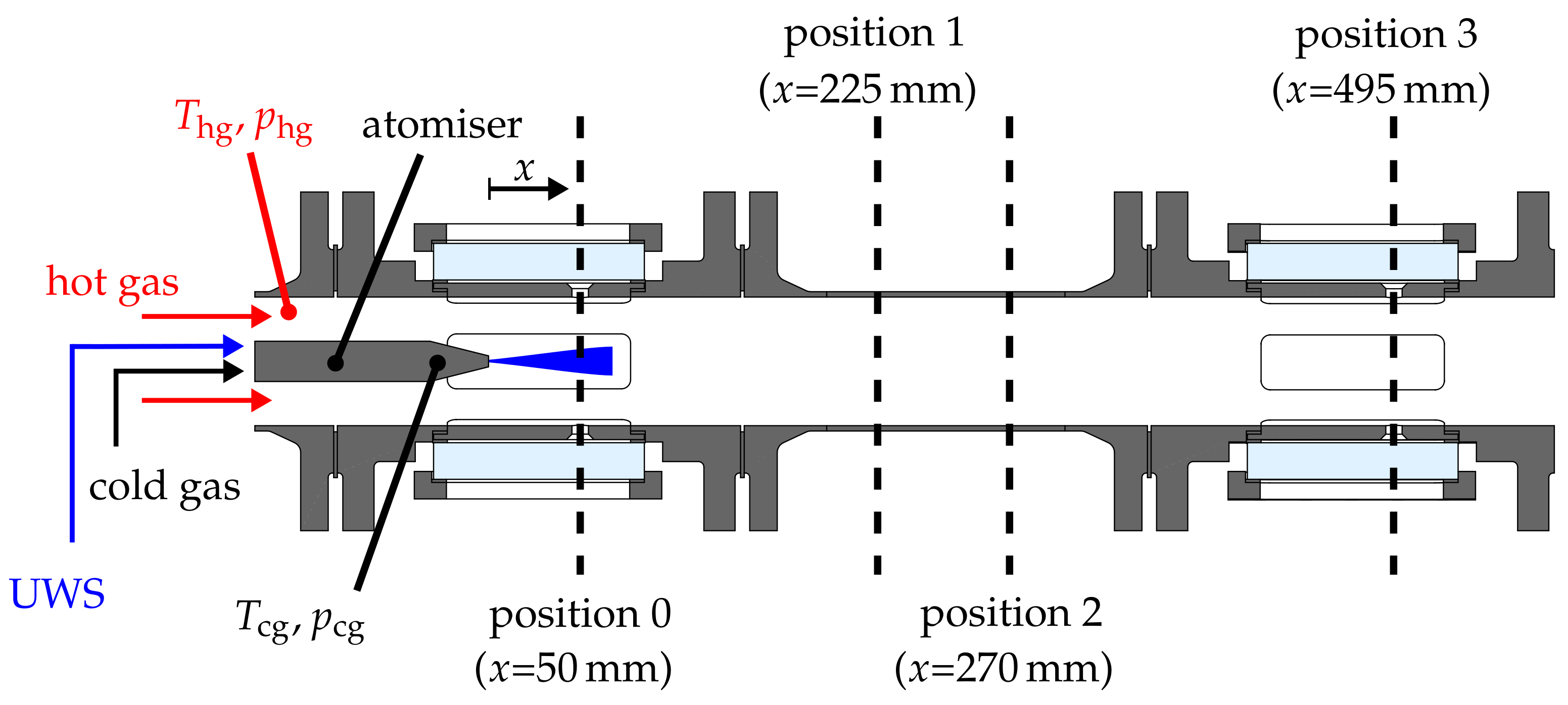
The subsequent discussion of the results is focused on the capabilities of the diagnostics. In this context, the first measurement position downstream of the atomiser (x = 50 mm) is of great importance for the methodology, since the droplet data recorded at this position can be utilised as droplet starting conditions for numerical simulations of spray evaporation. Hence, it must be ensured that sufficient information about the spray is captured in order to avoid inconclusive results.

Furthermore, the accuracy of measuring the gas velocity by using the smallest detectable droplets as seeding particles is assessed by a Stokes number analysis. The resulting gas velocity may yield important information for the analysis of spray systems, since the relative velocity of droplets with regard to the gas phase can be derived. Finally, it will be elucidated that the described methodology will provide experimental validation data, which can be used to study the evaporation characteristics of UWS under technical relevant flow conditions.

3.1. Spray Characteristics

An ambitious goal of numerous spray experiments is the detection of the spray characteristics like droplet diameter distribution or velocity profiles as close as possible to the atomiser. This is in particular important for an insight into the primary atomisation process or if the starting conditions of the droplets are sought for numerical simulations. The first measurement position of this study was placed 50 $\mathrm{m}$$\mathrm{m}$ downstream of the atomiser because secondary atomisation is almost completed at this position. On the other hand, an acceptable droplet concentration is present which facilitates post-processing. The results at this position reveal spray characteristics typical for the twin-fluid atomiser, which will be discussed in detail in the following.

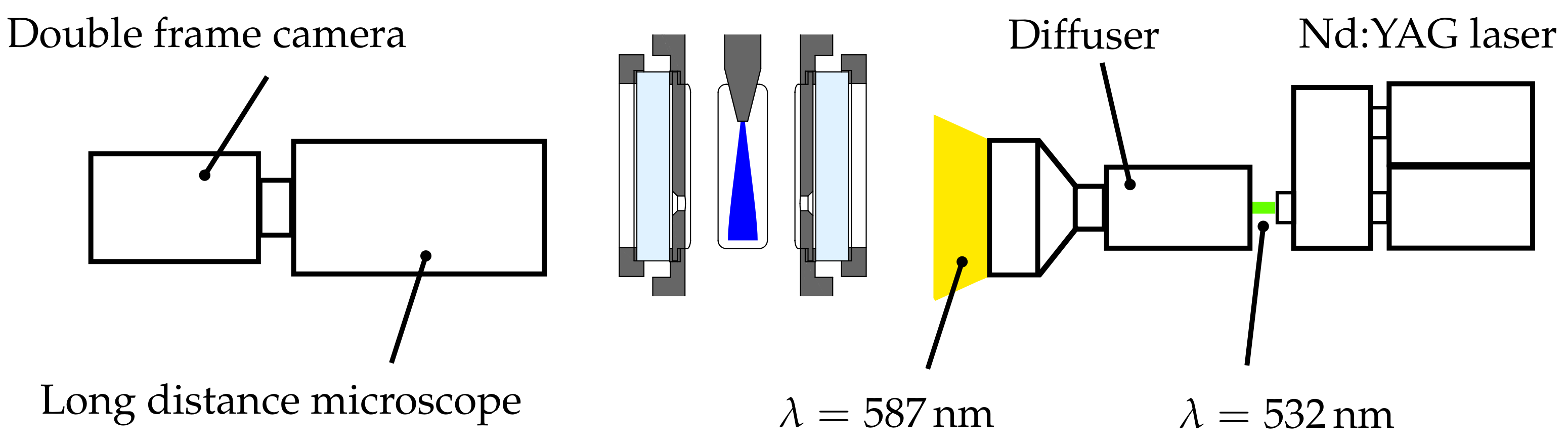
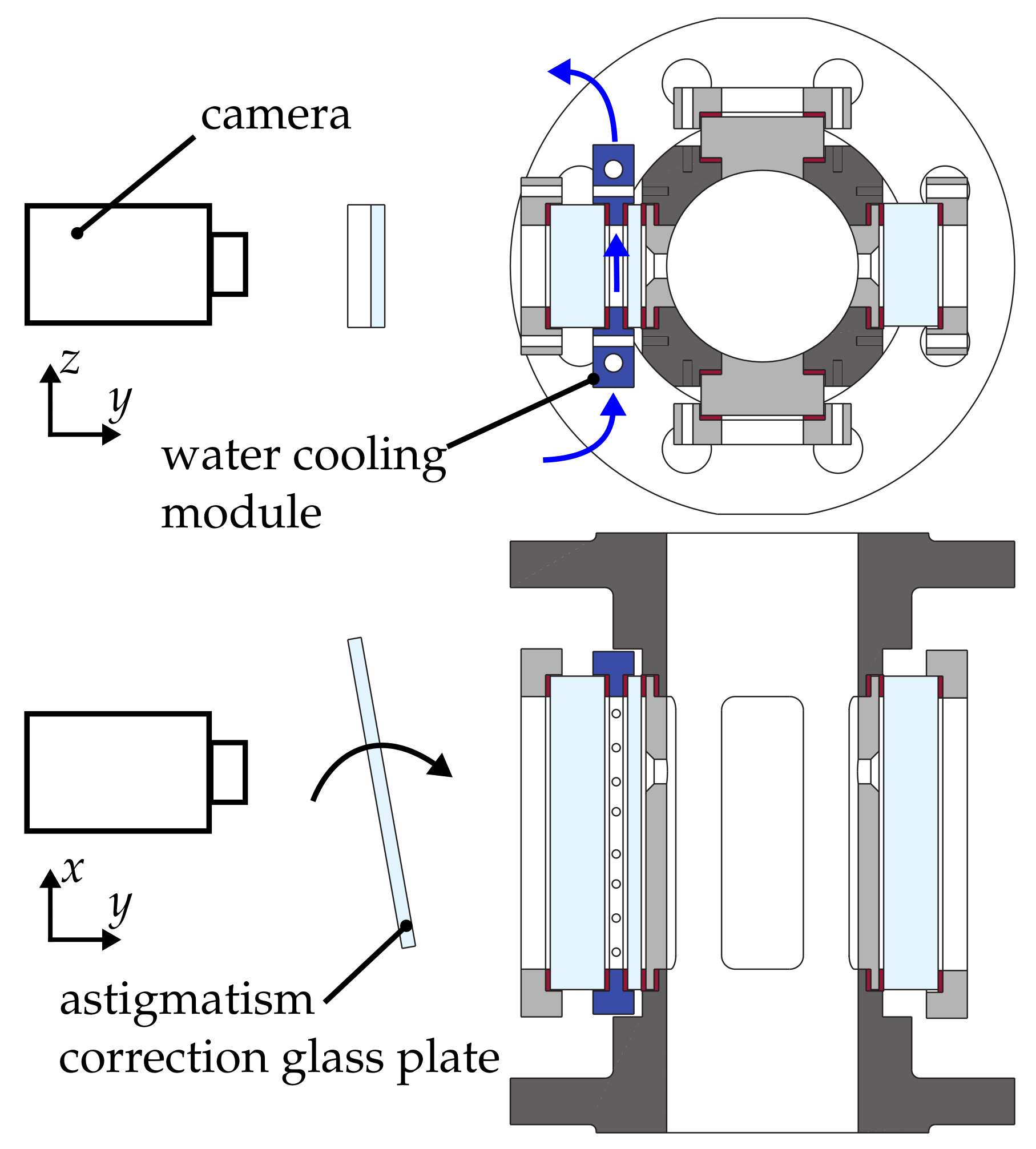
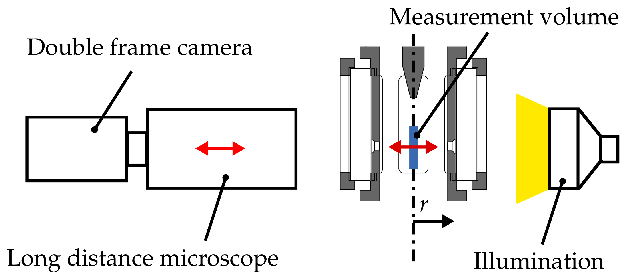
The present diagnostics offer the possibility to vary the position of the measurement volume across the cross section of the pipe by simply moving the camera in the direction of the optical axis as depicted in Figure 9. In this context, the small depth of field is a significant advantage of the present microscopic imaging setup, since a slim and thus well–defined measurement volume is achieved. 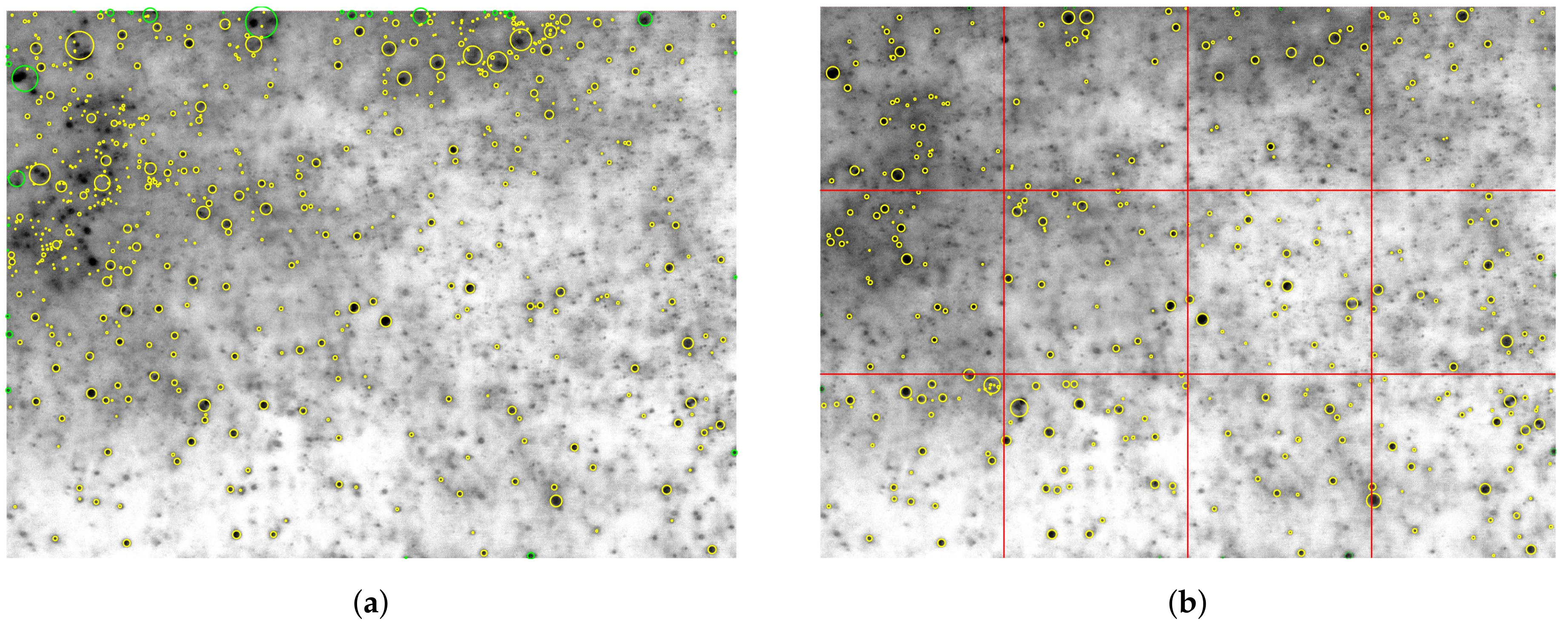Finally, a traversing of ±5 $\mathrm{m}$$\mathrm{m}$ in a radial direction around the centre of the pipe was employed covering 11 measurement positions. At each position, 3000 double frame images are taken with a repetition rate of 10 Hz. The resulting number of evaluated droplets varied from a few thousands at the edge to approximately 120,000 at the centre of the spray.

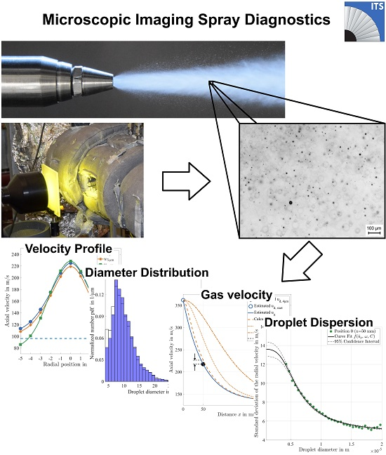
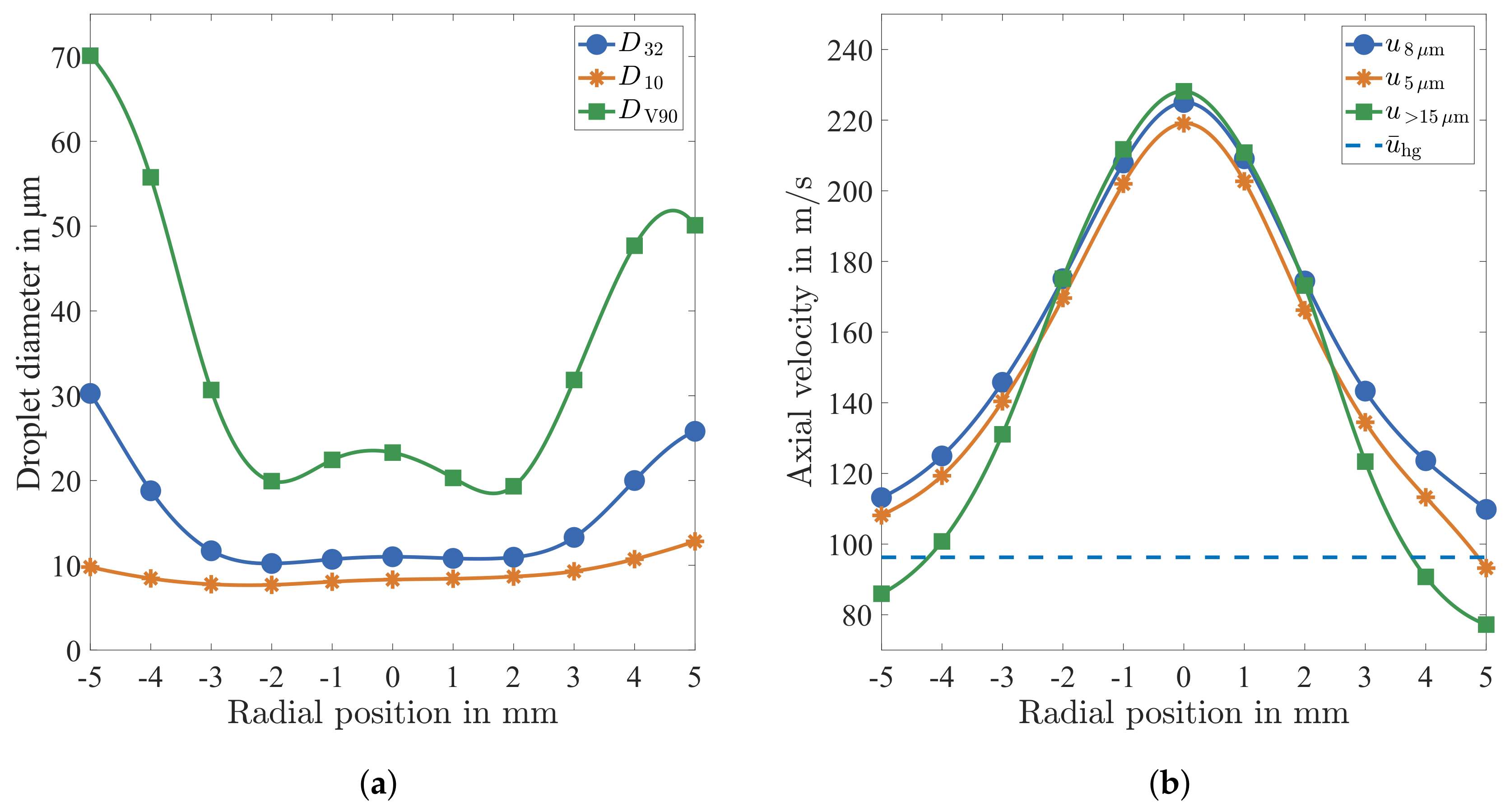
A typical result is plotted in Figure 10a in terms of characteristic droplet diameters. Obviously, the profiles are not perfectly symmetric. The reason for this phenomenon is assumed to result from some measurement positions featuring low statistical significance. First of all, it is found that the statistical significance is reduced with increased distance from the centre of the spray due to a lower concentration of droplets. Moreover, the high concentration of droplets at the centre of the spray causes a stronger background noise if the inner spray cone is situated between camera and measurement position. Hence, the outer positions in positive radial direction in Figure 10a are characterised by a lower signal-to-noise ratio, and therefore a lower quantity of droplets is evaluated. Speaking in numbers, at the extreme positions of +5 mm and −5 mm, approximately 4000 and approximately 19,000 droplets are detected, respectively. Nevertheless, the overall quantity of evaluated droplets is sufficient for a further analysis of the spray characteristics.

In general, the atomiser is capable of producing a very fine spray. The Sauter Mean Diameter $D_{32}$ stays at a constant level just above 10 $\mathsf{\mu }$$\mathrm{m}$ over a range of ±2 $\mathrm{m}$$\mathrm{m}$ in a radial direction. In this core zone large droplets, represented by the diameter at 90% volumetric quantile $D_{V90}$, have a diameter in the range of 20 to 25 $\mathsf{\mu }$$\mathrm{m}$. While the arithmetic mean Diameter $D_{10}$ yields no strong variation in a radial direction, a clear inhomogeneity is revealed by the profiles of $D_{32}$ and $D_{V90}$. Both characteristic diameters increase sharply at a distance of 2–3 $\mathrm{m}$$\mathrm{m}$ from the centre of the spray, which gives evidence to an imperfect atomisation process at the outer edge of the spray cone.

In addition to the information about droplet size, the velocity has been determined for each detected droplet. The result is summarised in Figure 10b by means of three average velocity profiles plotted over the radial direction of the pipe flow. The first profile ${\overline{u}}_{8\mathsf{\mu }\mathrm{m}}$ represents the average velocity of droplets of 8 $\mathsf{\mu }$$\mathrm{m}$ diameter, which is calculated for a diameter range of 8 ± $0.5$ $\mathsf{\mu }$$\mathrm{m}$ in order to achieve statistical significance. At the centre of the spray, a very high velocity is detected, which is far above the bulk velocity of the gas phase ${\overline{u}}_{\mathrm{hg}}$ = 96 $\mathrm{m}{\mathrm{s}}^{-1}$. This is caused by the high velocity of the air stream emerging from the nozzle. At the edge of the traverse displacement, the velocity drops down to slightly above the bulk velocity of the gas phase. The reason for this behaviour is given by the slower bulk hot gas flow, which decelerates the air flow from the nozzle. In this context, it should be noted that the outlet bore hole diameter of the atomiser nozzle is 2 $\mathrm{m}$$\mathrm{m}$.

The velocity ${\overline{u}}_{5\mathsf{\mu }\mathrm{m}}$ of droplets of 5 $\mathsf{\mu }$$\mathrm{m}$ diameter was found to be lower than ${\overline{u}}_{8\mathsf{\mu }\mathrm{m}}$ over the entire profile due to the lower inertia of the smaller droplets. Similarly, the velocity of droplets of a diameter greater than 15 $\mathsf{\mu }$$\mathrm{m}$${\overline{u}}_{>15\mathsf{\mu }\mathrm{m}}$ is presumed to feature the fastest velocity over the entire radial dimension. In contrast, ${\overline{u}}_{>15\mathsf{\mu }\mathrm{m}}$ was found to have the fastest velocity only at the centre region of the spray. It shows a strong decrease towards the edges of spray, where the lowest velocity of the three velocity profiles is measured. In this region, ${\overline{u}}_{>15\mathsf{\mu }\mathrm{m}}$ even drops below the bulk velocity of the gas flow. A possible explanation for this effect may be derived from the diameter distribution in Figure 10a. These results indicate an imperfect atomisation at the outer edge of the spray, which may lead to larger droplets emerging with low initial velocity from the atomiser.

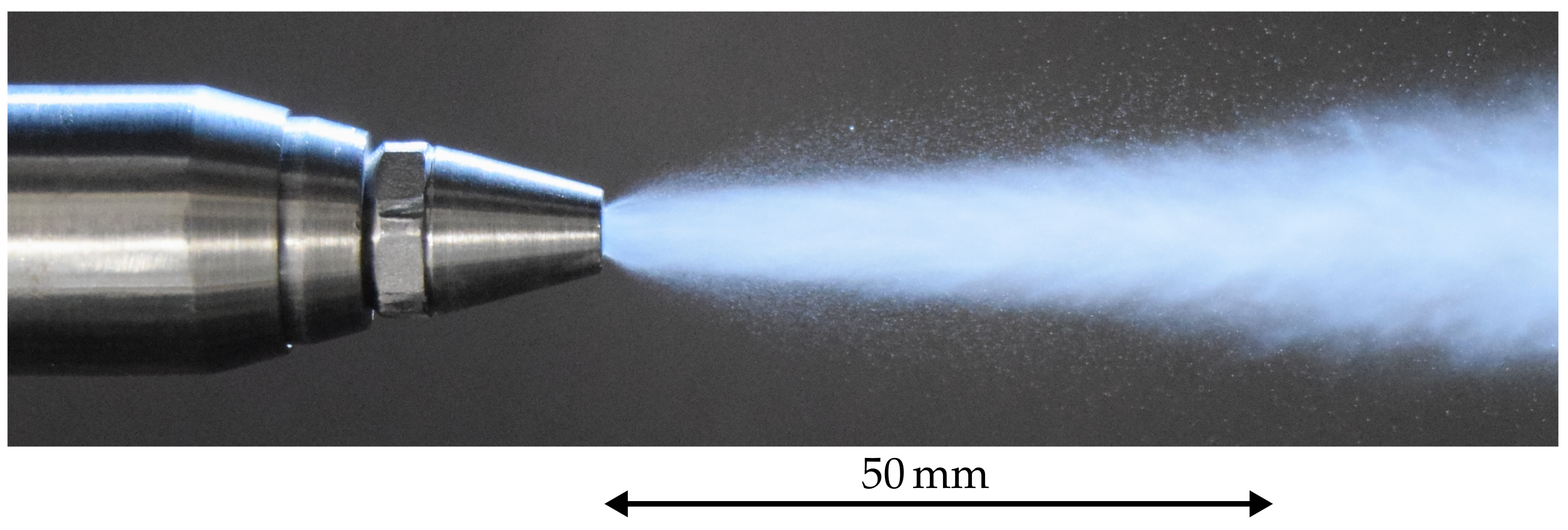
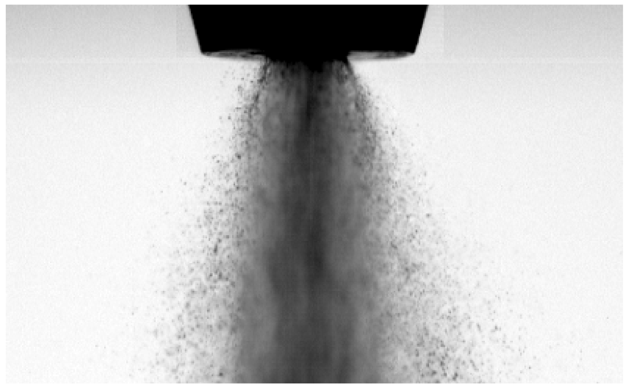
A snapshot of the spray in the near nozzle region was recorded using a relatively long exposure time of approximately $0.14$ $\mathrm{m}$s as shown in Figure 11. Obviously, the centre of the spray can not be investigated in detail due to motion blur. In contrast to that, droplets at the outer region of the spray as well as liquid structures still connected to the atomiser nozzle are recorded sharply, which implies that they feature a considerably lower velocity in comparison to droplets within the main spray cone. Therefore, the statement of large droplets with low initial velocity is confirmed, which is also in accordance with the general primary atomisation process of an effervescent atomiser as reviewed by Sovani et al. [39].

The radial position featuring the strongest velocity gradient of all velocity profiles in Figure 10b, approximately $2 \mathrm{m}\mathrm{m}$ off the centre, represents the shear layer zone between the jet flow of the atomiser and the surrounding hot gas flow. In this region, the finest spray is recorded as illustrated by the $D_{32}$ and in particular by the $D_{V90}$. Both characteristic diameters increase sharply at a further distance from the centre of the spray. This behaviour may be caused by the strong velocity gradient in combination with shear layer turbulence. Hence, the atomisation process in this region is dominated by the resulting high relative velocity between the droplets and the hot gas. At this point, it should be emphasised that the evaluation of this correlation between droplet size and velocity is only possible because the diagnostics is capable of detecting the size and velocity of individual droplets.

In conclusion, these initial results of the test section comprise important spray data close to the atomiser. In particular, the possibility to obtain data at different positions in a radial direction in a dense spray region turns out to be a great advantage of the measurement technique. This gives a better understanding of the atomisation process or enables the tuning of the cold gas mass flow of the atomiser ${\dot{m}}_{\mathrm{cg}}$ in order to achieve desired spray characteristics. Furthermore, the recorded data in the proximity of the atomiser can be utilised as droplet starting conditions for numerical simulations of spray evaporation. In this context, the captured inhomogeneities of the droplet diameter and velocity profiles represent vital input data for numerical predictions.

3.2. Determining the Gas Velocity

The gas velocity is an important parameter for the analysis of spray systems, since the relative velocity of droplets to the gas flow can be derived. This relative velocity, which is also called slip velocity, has a strong influence on droplet kinematics, secondary atomisation, and evaporation [2]. Hence, the simultaneous measurement of gas and droplet velocity is a great advantage for spray diagnostics. Standard optical techniques for measuring the gas velocity are Laser Doppler Anemometry (LDA) and Particle Image Velocimetry (PIV). Both techniques require seeding the flow with small particles in the order of 1 $\mathsf{\mu }$$\mathrm{m}$ in diameter. These seeding particles will follow the flow almost perfectly due to their low inertia.

Microscopic imaging has already been demonstrated to be capable to detect such seeding particles if the droplet size is not of interest using Particle Shadow Velocimetry [40]. In addition to an often simpler optical setup, this technique can be advantageous in comparison to established diagnostics like PIV or LDA for small-scale applications or multiphase flows [41,42]. However, the goal of this study is to detect not only the velocity, but also the diameter of individual droplets.

Therefore, one way to realise a simultaneous measurement of gas and droplet velocity is the utilisation of the smallest detectable droplets as seeding particles. Hence, no additional seeding is necessary and the non-intrusive and simultaneous measurement of the gaseous velocity field is possible as long as enough small droplets are present in the flow. This methodology was successfully applied with the PDA for detecting evaporating [31] and burning droplets [32]. In these studies, droplets of a size smaller than 3–5 $\mathsf{\mu }$$\mathrm{m}$ were utilised to derive the gas velocity.

The present microscopic imaging setup also offers the possibility to detect droplets of such small size, which may be utilised as seeding. However, it is mandatory that the droplets of a selected size do follow the flow correctly in order to derive a sensible gas velocity. In this context, it is important to note that the droplet size cannot be specified in advance since it depends on the actual flow field of the gas. Subsequently, the timescales due to the inertia of the droplets will be estimated in order to decide up to which size the droplets are suitable as tracers of the gas flow. This gives a measure of the accuracy of the present diagnostics for determining the gas velocity.

The following estimation will focus on the most critical part of the flow field of the experimental setup in this study: the strong deceleration of the air jet emerging from the atomiser nozzle. First of all, a Stokes flow is assumed for the gas flow around the droplet [43]. The relevant timescale is the response or relaxation time of a droplet

$${\tau }_{\mathrm{d}}=\frac{{\rho }_{\mathrm{d}}{D}_{\mathrm{d}}^2}{18{\mathsf{\mu }}_{\mathrm{g}}},$$

(3)

which is dependent on the density of the droplet ${\rho }_{\mathrm{d}}$, the droplet diameter $D_{\mathrm{d}}$ and the dynamic viscosity of the gas ${\mathsf{\mu }}_{\mathrm{g}}$. Considering the relative velocity between droplet and the gas phase $(u_{\mathrm{g}}\left(t\right)-u_{\mathrm{d}}\left(t\right))$ and neglecting gravitation, the equation of motion can be written as

$$\frac{\mathrm{d}{u}_{\mathrm{d}}}{\mathrm{d}t}=\frac{1}{{\tau }_{\mathrm{d}}}(u_{\mathrm{g}}\left(t\right)-u_{\mathrm{d}}\left(t\right)).$$

(4)

Taking the homogeneous solution of this differential equation, it is obvious that the droplet velocity recovers after a sudden jump according to

$$u_{\mathrm{d}}\left(t\right)\sim e^{-\frac{t}{{\tau }_{\mathrm{d}}}}.$$

(5)

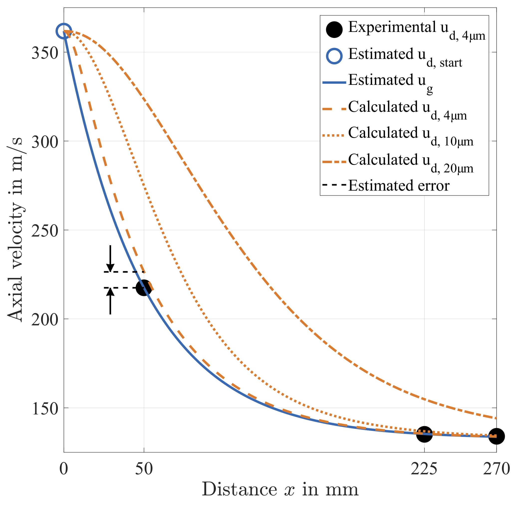
The determination of an appropriate timescale of the gaseous phase is not straightforward, since it depends on the actual flow field. As a first approach, the assumption is made that the axial velocity of the droplets of 4 $\mathsf{\mu }$$\mathrm{m}$ diameter $u_{\mathrm{d},4\mathsf{\mu }\mathrm{m}}\left(t\right)$ represents the velocity of the gas phase. The experimental results of the temporal arithmetic mean of $u_{\mathrm{d},4\mathsf{\mu }\mathrm{m}}\left(x\right)$ at the centre of the pipe are illustrated in Figure 12 for the first three measurement positions downstream of the atomiser.

However, the initial velocity of the gas and the droplets at the atomiser exit is not available. Furthermore, the evolution of the velocity directly downstream of the nozzle is governed by gas dynamics and the resulting primary atomisation. In this study, the initial velocity of the droplets and the air is estimated as $\mathrm{Ma}=1$ at the nozzle outlet based on the estimated droplet starting temperature $T_{\mathrm{d}0}$. The present atomiser is operated at supercritical flow conditions in order to achieve a strong pressure drop at the atomiser outlet. Hence, this assumption is reasonable. Furthermore, the assumption is conservative in terms of the estimation of the measurement accuracy, since expected shock waves may lead to a lower effective initial velocity of droplets after primary atomisation in the near nozzle region.

In the next step, a function of the type

$$u_{\mathrm{g}}\left(t\right)=C_1{e}^{-\frac{t}{{\tau }_{\mathrm{g}}}}+C_2$$

(6)

is used to fit the estimated and experimental data in order to derive an estimated evolution of the gas velocity $u_{\mathrm{g}}$, which is shown in Figure 12. This function is chosen according to Equation (5). Hence, a timescale of the gas phase ${\tau }_{\mathrm{g}}$ can be derived and the Stokes number of a droplet with a diameter of 4 $\mathsf{\mu }$$\mathrm{m}$ can be calculated:

$${\mathrm{St}}_{4\mathsf{\mu }\mathrm{m}}=\frac{{\tau }_{\mathrm{d}}}{{\tau }_{\mathrm{g}}}=0.13.$$

(7)

Since the condition,

$${\mathrm{St}}_{4\mathsf{\mu }\mathrm{m}}\ll 1,$$

(8)

is not perfectly fulfilled, the derived evolution of the gas velocity is used to solve a more generalised equation of motion of one droplet,

$$\frac{\mathrm{d}{u}_{\mathrm{d}}}{\mathrm{d}t}=-\frac{3}{4}\frac{{\rho }_g{c}_D}{{\rho }_d{D}_d}|u_{\mathrm{g}}\left(t\right)-u_{\mathrm{d}}\left(t\right)|(u_{\mathrm{g}}\left(t\right)-u_{\mathrm{d}}\left(t\right)),$$

(9)

in order to estimate the measurement accuracy. The correlation of Ihme et al. [44] is used to determine the drag coefficient

$$c_D=0.36+5.48R{e}_d^{-0.573}\frac{24}{R{e}_d}.$$

(10)

This correlation is only valid for perfect spheres, which is a reasonable assumption for the small droplets in this study. Most importantly, Equation (10) was validated experimentally for droplet Reynolds numbers

$$R{e}_d=\frac{D_d|u_{\mathrm{g}}\left(t\right)-u_{\mathrm{d}}\left(t\right)|}{{\nu }_{\mathrm{hg}}}<{10}^4.$$

(11)

Therefore, the main restriction of the Stokes theory ($R{e}_d<1$) is overcome. The resulting spatial evolution of the velocity of a droplet of a diameter of 4 $\mathsf{\mu }$$\mathrm{m}$ $u_{\mathrm{d},4\mathsf{\mu }\mathrm{m}}\left(x\right)$ is illustrated in Figure 12. Obviously, droplets of a diameter of 4 $\mathsf{\mu }$$\mathrm{m}$ follow the estimated gas velocity very well. Furthermore, this approach yields directly the estimated measurement error at position 0 at a distance of $x_0$ = 50 $\mathrm{m}$$\mathrm{m}$ downstream of the atomiser:

$$\frac{u_{\mathrm{d},4\mathsf{\mu }\mathrm{m}}\left(x_0\right)-u_{\mathrm{g}}\left(x_0\right)}{u_{\mathrm{g}}\left(x_0\right)}=\frac{8.94\mathrm{m} {\mathrm{s}}^{-1}}{217.5\mathrm{m} {\mathrm{s}}^{-1}}=4.1\%.$$

(12)

In view of the strong estimated deceleration at the near-nozzle region, the measurement accuracy is acceptable. Furthermore, an iterative determination of $u_{\mathrm{g}}$ is possible based on the already obtained results. This way, $u_{\mathrm{g}}$ can be determined with improved accuracy. In the scope of this paper, however, the gas velocity is simply taken from the velocity of the smallest detectable droplets. Additionally, the response of droplets of 10 $\mathsf{\mu }$$\mathrm{m}$ and 20 $\mathsf{\mu }$$\mathrm{m}$ diameter is calculated, which corresponds to the smallest detectable droplet range of non-microscopic imaging techniques. Both results are plotted in Figure 12 and reveal a drastically greater measurement error than that of the 4 $\mathsf{\mu }$$\mathrm{m}$ droplets, which emphasizes the specific advantage of the method.

In summary, the use of microscopic imaging seems to be well suited for determining the gas velocity by using the velocity of the smallest detectable droplets. This is advantageous as no additional input is required, neither regarding the experimental setup nor with respect to the processing routine. The additional information about the gas flow field can be utilised to analyse and validate droplet kinematics. In addition, the effect of the slip velocity on secondary atomisation or evaporation can be evaluated.

3.3. Discussion of Velocity Fluctuations

Since the temporal average of the gas velocity can be derived with sufficient accuracy, the discussion is extended to the statistical analysis of velocity fluctuations. This requires the post-processing, as presented in Section 2.3, to be extended in order to exclude spurious vector assignments, which may compromise the statistical analysis. The universal outlier detection of Westerweel and Scarano [45] is widely used for Particle Image Velocimetry (PIV) data. This technique is based on a normalised median filter, which considers the neighbour velocity vectors of the vector under concern. Furthermore, this filter was verified for a wide range of Reynolds numbers ranging from ${10}^{-1}$ to ${10}^7$. In contrast to PIV data, Particle Tracking Velocimetry (PTV) yields non-equidistant neighbour vectors. Hence, a weighting of neighbour vectors based on the distance from the droplet velocity vector concerned is used as proposed by Duncan et al. [46]. Finally, this filter is applied using a conservative threshold of 2 to ensure that spurious vectors are effectively removed.

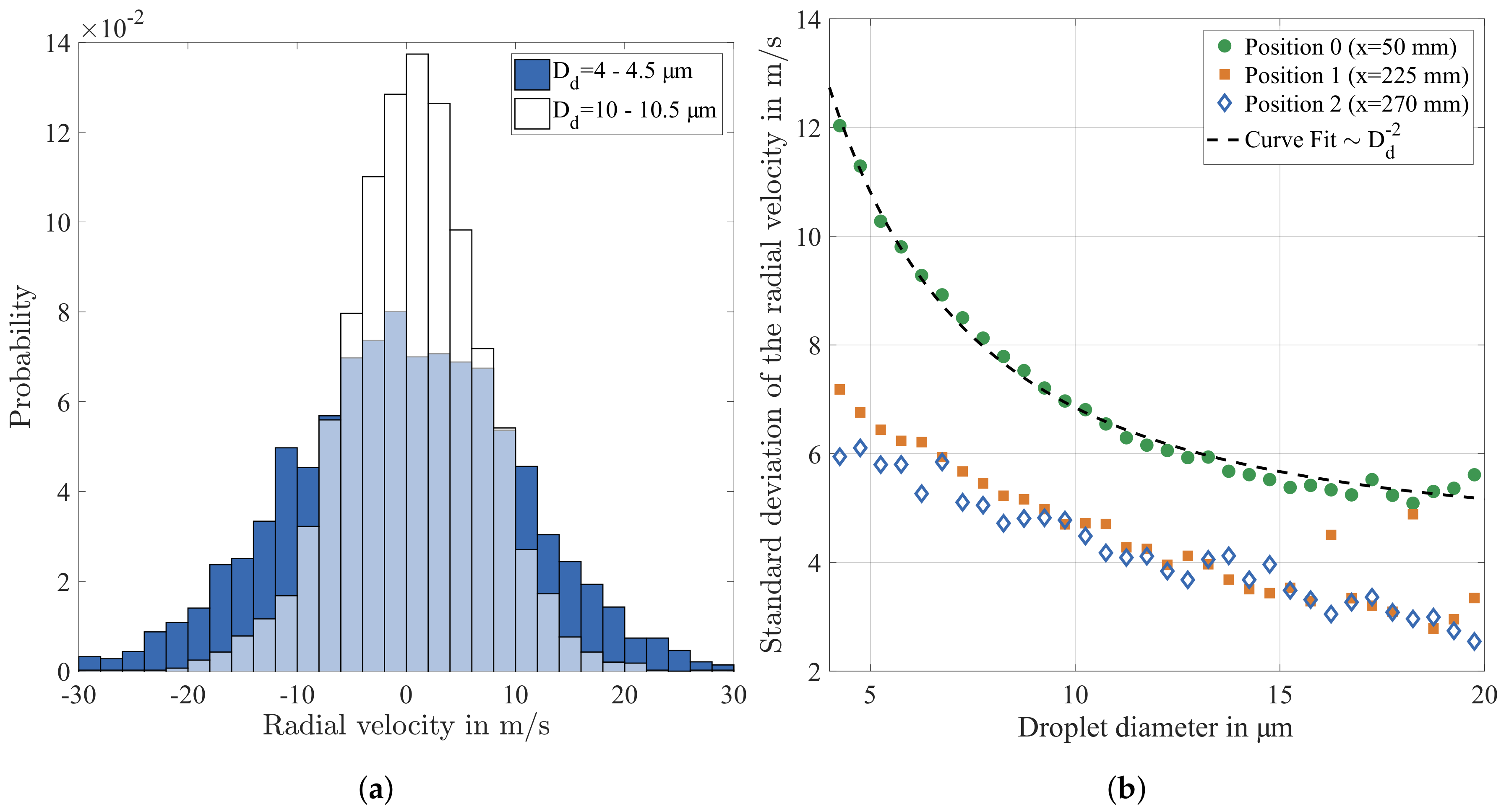
The droplet data at specific spatial positions are split into droplet diameter classes with a constant width of $0.5$ $\mathsf{\mu }$$\mathrm{m}$ in order to evaluate the effect of droplet size on velocity fluctuations. The probability distribution of the radial velocity is illustrated exemplarily for two droplet diameter classes at a distance of x = 50 mm downstream of the atomiser in Figure 13a. Obviously, this velocity component is normally distributed and the mean value is approximately 0 $\mathrm{m}{\mathrm{s}}^{-1}$. Furthermore, the radial velocity of the smaller droplets has a higher standard deviation, which may indicate that those droplets follow the velocity fluctuations of the gas phase considerably better compared to larger ones.

For a more detailed analysis, the standard deviation of the radial velocity is calculated for each droplet diameter class in the range between 4 $\mathsf{\mu }$$\mathrm{m}$ and 20 $\mathsf{\mu }$$\mathrm{m}$. The result reveals a decreasing standard deviation with increasing droplet diameter at all positions downstream of the atomiser as shown in Figure 13b. The most interesting observation is that, at the position closest to the atomiser nozzle (x = 50 mm), the standard deviation of the radial velocity is found to be proportional to $D_{\mathrm{d}}^{-2}$. Considering the timescale of droplet relaxation, as indicated by Equation (3), there is strong evidence that the standard deviation of the droplet velocity is due to the fluctuations of the gas velocity.

Hence, the generally high standard deviation at position 0 obviously results from strong turbulent fluctuations of the gas phase. At this measurement position, a strong shear layer turbulence is generated by the interaction of the rapid cold gas injected by the atomiser with the substantially slower hot gas flow. This result is supported by the strong gradient of the axial droplet velocity as shown in Figure 10b. The positions further downstream of the atomiser are characterised by a generally lower level of the standard deviation and a considerably weaker dependency on droplet size. This result is sensible, since the influence of the atomiser air flow and the resulting shear layer turbulence decays with increasing distance downstream of the atomiser.

The standard deviation of the radial velocity, as shown in Figure 13b, represents a valuable result, since it can be directly applied for predicting the turbulent dispersion. Consequently, the droplet trajectories in the test section can be computed dependent on the droplet size. In addition, the standard deviation of the velocity may contain vital information about the turbulent fluctuations of the gas phase. These velocity fluctuations impose an additional relative velocity between droplets and gas, which may affect evaporation or atomisation considerably. In literature, high–spatial–resolution PIV is presented as a promising technique for investigation of turbulent fluctuations in dispersed multiphase flows [33].

Subsequently, it will be investigated whether an estimation of the turbulent fluctuations of the gas phase or even the turbulent slip velocity is possible based on the present microscopic imaging data. First of all, the theoretical analysis of particle response in an oscillating gas phase presented by Burger et al. [47] is adapted to turbulent fluctuations. The turbulent gas velocity is simplified by a simple sinusoidal oscillation

$$u_{\mathrm{g}}={\overline{u}}_{\mathrm{g}}+{\widehat{u}}_{\mathrm{g}}sin\omega t,$$

(13)

which is defined by the amplitude ${\widehat{u}}_{\mathrm{g}}$ and the angular frequency $\omega$. The mean velocity ${\overline{u}}_{\mathrm{g}}$ is set to 0 $\mathrm{m}{\mathrm{s}}^{-1}$. Stokes flow is assumed analogous to the analysis of the mean gas velocity. By inserting Equation (13) into Equation (4), the oscillation of the droplet velocity after reaching the steady-state condition can be derived

$$u_{\mathrm{d}}=\frac{{\widehat{u}}_{\mathrm{g}}}{\sqrt{1+{\tau }_{\mathrm{d}}^2{\omega }^2}}sin\left(\omega t+arctan\left({\tau }_{\mathrm{d}}\omega \right)\right).$$

(14)

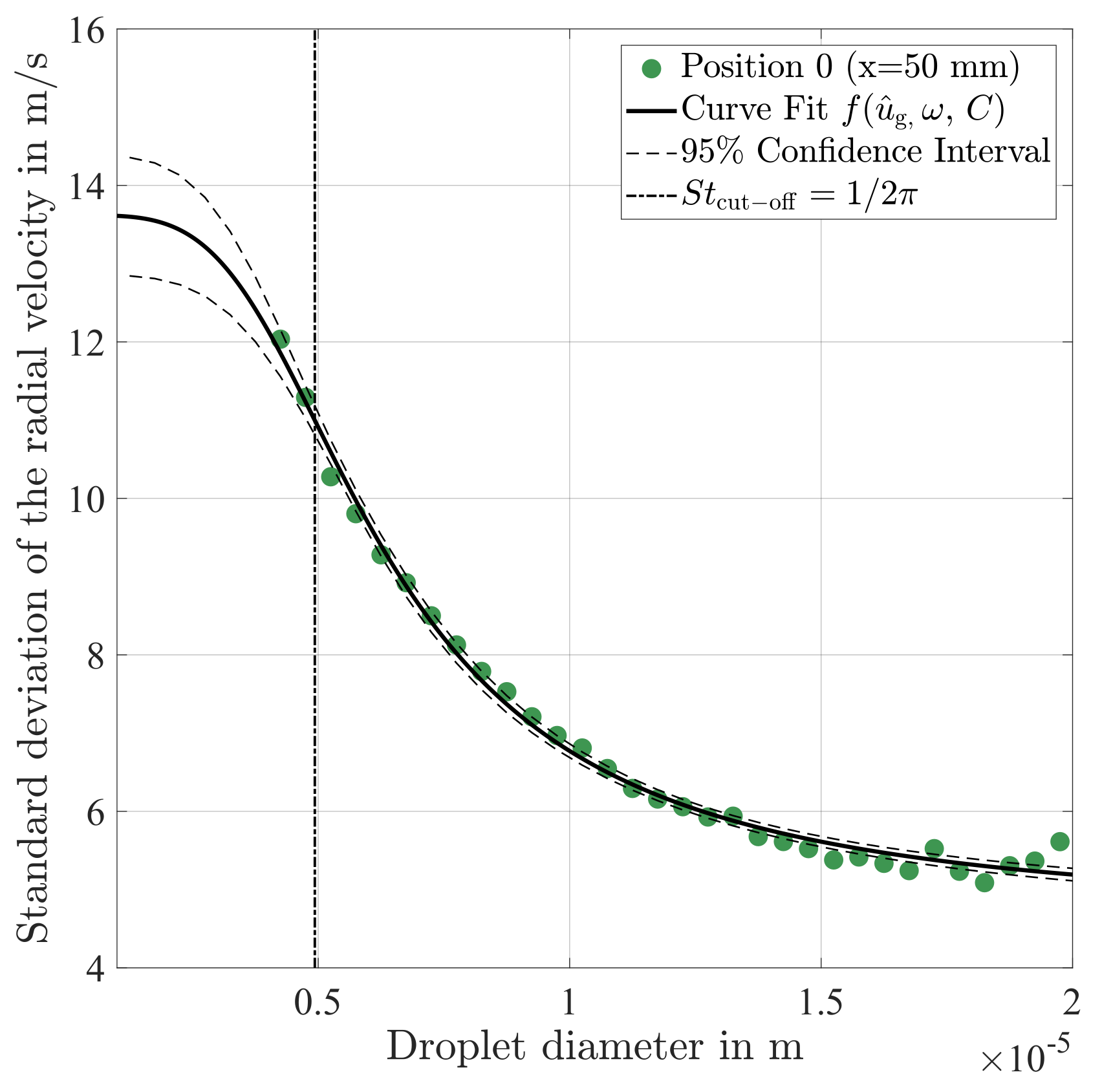
In this study, only the amplitude of the resulting droplet velocity oscillation is of interest. Hence, the function

$$f({\widehat{u}}_g,\omega ,C)=\frac{1}{\sqrt{2}}\left(\frac{{\widehat{u}}_{\mathrm{g}}}{\sqrt{1+{\tau }_{\mathrm{d}}^2{\omega }^2}}+C\right)$$

(15)

is employed for fitting the experimental data. The amplitude is scaled by the factor $\frac{1}{\sqrt{2}}$ in order to enable a direct comparison to the experimentally available standard deviation. Furthermore, the desired dependency of this amplitude function on the droplet diameter is represented by the droplet relaxation time ${\tau }_{\mathrm{d}}$, which is affected additionally by the density of the droplets ${\rho }_{\mathrm{d}}$ and the dynamic viscosity of the gas phase ${\mathsf{\mu }}_{\mathrm{g}}$. The constant C was found to be necessary in order to achieve a sensible fit. This offset is supposed to result from fluctuations of the gas velocity, which are characterised by lower frequencies. Hence, all droplets in the presented size range are assumed to follow those low frequency fluctuations almost perfectly.

The fit of $f({\widehat{u}}_{\mathrm{g}},\omega ,C)$ from Equation (15) is found to be in excellent agreement to the experimental data as shown in Figure 14. The desired information about the underlying oscillation by means of ${\widehat{u}}_{\mathrm{g}}$ and $\omega$ can be estimated with reasonable accuracy, which is graphically illustrated by 95% confidence intervals for the fitted function. In addition, the resulting parameters of $f({\widehat{u}}_{\mathrm{g}},\omega ,C)$ are summarised in

Table 3. Estimated properties of the turbulent fluctuations of the gas phase by fitting $f({\widehat{u}}_{\mathrm{g}},\omega ,C)$ to experimental data. The indicated uncertainty is based on a 95% confidence interval.

Parameter	Symbol	Value
Amplitude	${\widehat{u}}_{\mathrm{g}}$	$12.7$ ± $1.0$ $\mathrm{m}{\mathrm{s}}^{-1}$
Angular frequency	$\omega$	$27.0$ ± $3.8$ $\mathrm{k}$Hz
Frequency	f	$4.3$ ± $0.6$ $\mathrm{k}$Hz
Constant offset	C	$6.6$ ± $0.1$ $\mathrm{m}{\mathrm{s}}^{-1}$

.

The cut-off Stokes number

$$S{t}_{\mathrm{cut}}-\mathrm{off}={\tau }_{\mathrm{d}}f={\displaystyle \frac{1}{2\pi }}$$

(16)

can be determined using the derived frequency of the oscillation f, as fundamentally introduced in work of Burger et al. [47] for studying the particle response in oscillating flows. This cut-off Stokes number may be used analogous to the cut-off frequency of a first order low pass filter in order to assign different regimes of droplet motion in a turbulent gas flow. In the case under consideration, the droplet diameter of $4.9$ $\mathsf{\mu }$$\mathrm{m}$ is determined using Equation (16), which is graphically illustrated in Figure 14. Hence, the droplets in this size range can be used as an indicator for turbulent fluctuations of the gas phase. Subsequently, this will be demonstrated based on a more detailed analysis of the spray characteristics at Position 0 (x = 50 mm).

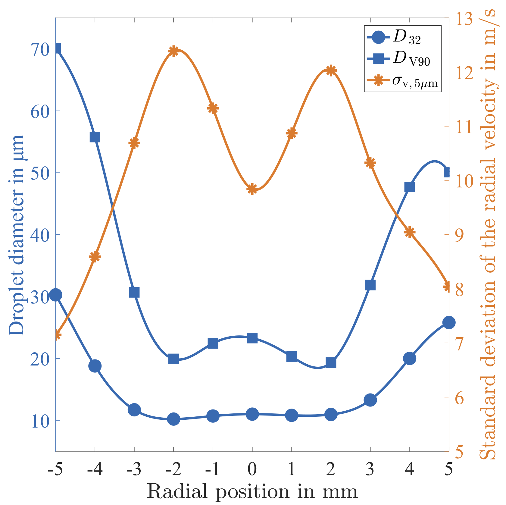
In Figure 15, the Sauter Mean Diameter ($D_{32}$) and the diameter at the 90% volumetric quantile ($D_{\mathrm{V}90}$) are plotted over the radial position. These results were already discussed in Section 3.1. In particular, the radial positions featuring the strongest average velocity gradient, ± 2 mm off the centre, were found to correspond to the smallest characteristic diameters. Therefore, shear layer turbulence seems to play a major role during the atomisation process.

For a further in depth analysis, the standard deviation of the radial velocity of very small droplets is discussed. The standard deviation ${\sigma }_{\mathrm{v}},5 \mathsf{\mu }\mathrm{m}$ is plotted in Figure 15, which is determined using droplets of a diameter between $4.5$ $\mathsf{\mu }$$\mathrm{m}$ and $5.5$ $\mathsf{\mu }$$\mathrm{m}$. The distribution of ${\sigma }_{\mathrm{v}},5 \mathsf{\mu }\mathrm{m}$ is found to peak exactly at ± 2 mm off the centre, which confirms the statement that these regions correspond to strong velocity fluctuations caused by shear layer turbulence. Furthermore, the largest droplets of the spray, as represented by the $D_{\mathrm{V}90}$, are strongly correlated to ${\sigma }_{\mathrm{v}},5 \mathsf{\mu }\mathrm{m}$. Obviously, the turbulent fluctuations of the hot gas flow induce the dominating slip velocity, which triggers the atomisation process.

In conclusion, the standard deviation of the radial velocity directly yields an estimation of droplet dispersion, which can be utilised to validate the droplet distribution in the pipe flow as a function of the droplet size. Furthermore, information about the underlying turbulent fluctuations can be estimated with reasonable accuracy. Hence, the smallest detectable droplets may be used as an indicator for turbulence intensity.

However, the knowledge of the turbulent fluctuations does not directly yield the turbulent slip velocity of the droplets. Actually, the gradient of the mean velocity in an axial direction needs to be taken into account as well, since a small displacement in a radial direction due to turbulent dispersion may induce a high slip velocity in an axial direction as discussed by Chen et al. [31]. Hence, turbulent fluctuations may cause a high slip velocity of relatively small droplets, which are characterised by strong dispersion due to their low inertia. This effect needs to be considered in order to estimate an absolute slip velocity caused by turbulent fluctuations. However, a more detailed analysis of this slip velocity is beyond the scope of this paper.

As an outlook, if a high speed camera in combination with a suitable illumination is used, time-dependent droplet data can be recorded, which may give a more detailed insight into the interaction of the spray with turbulent fluctuations of the gas phase.

3.4. Evaporation Characteristics of Urea–Water Solution

The long-term objective of the present methodology is to provide experimental validation data, which can be used to study evaporating urea–water sprays under realistic thermodynamic conditions. In order to pin down the effect of urea on the evaporation process, distilled water is used as an alternative liquid in the measurement campaign. First of all, there is almost no difference in surface tension and viscosity between water and urea–water solution (UWS). Hence, it is presumed that the atomisation process is effectively not affected when using an air assisted nozzle. Therefore, it is expected that the same spray for UWS and water is generated.

However, a recent publication by Kapusta et al. [26] indicates that replacing UWS with water will influence the spray characteristics considerably. In this study, a pressure driven single fluid nozzle is used and the pressure in the liquid reservoir is preserved. In other words, the pressure difference over the whole injection system is kept constant. Therefore, the liquid volume flow through the atomiser may be affected by the fluid properties, most importantly by the viscosity. Hence, the velocity at the exit of the atomiser nozzle will also be affected, which is one major parameter affecting the primary breakup regime of a cylindrical jet. For the discussion of the effect of the Weber and Ohnesorge number, please refer to the review of Dumouchel [48]. In conclusion, the study of Kapusta et al. [26] does not evaluate the influence of different fluid properties on the actual atomisation process but on the performance of a whole injection system.

In contrast, an air assisted nozzle is used in the present study with an identical setting of the air mass flow and velocity, when replacing UWS with pure water. In addition, the liquid volume flow was kept identical. These provisions ensure that the relevant non-dimensional numbers are effectively identical for UWS and pure water. Therefore, the influence of slightly different liquid properties is considerably lower in comparison to simple pressure atomisers.

It should be noted that the density difference between UWS and water of approximately 9% will affect the integral momentum of the spray jet. However, this effect is negligible using a twin-fluid atomiser. Hence, the overall effect of different fluid properties for UWS and water on the atomisation process can definitely be considered as marginal. In summary, the present experimental configuration provides identical droplet initial conditions, since the atomiser produces practically the same spray for UWS and water. By this means, experimental results for water can be used to calibrate numerical simulations in terms of starting conditions and the quality of submodels, since the complex evaporation behaviour of UWS can be excluded. Furthermore, the comparison of droplet diameter distributions of UWS and water further downstream of the atomiser may provide insights in the evaporation behaviour of UWS. Subsequently, it will be evaluated if evaporation characteristics can be retrieved using the present microscopic imaging technique.

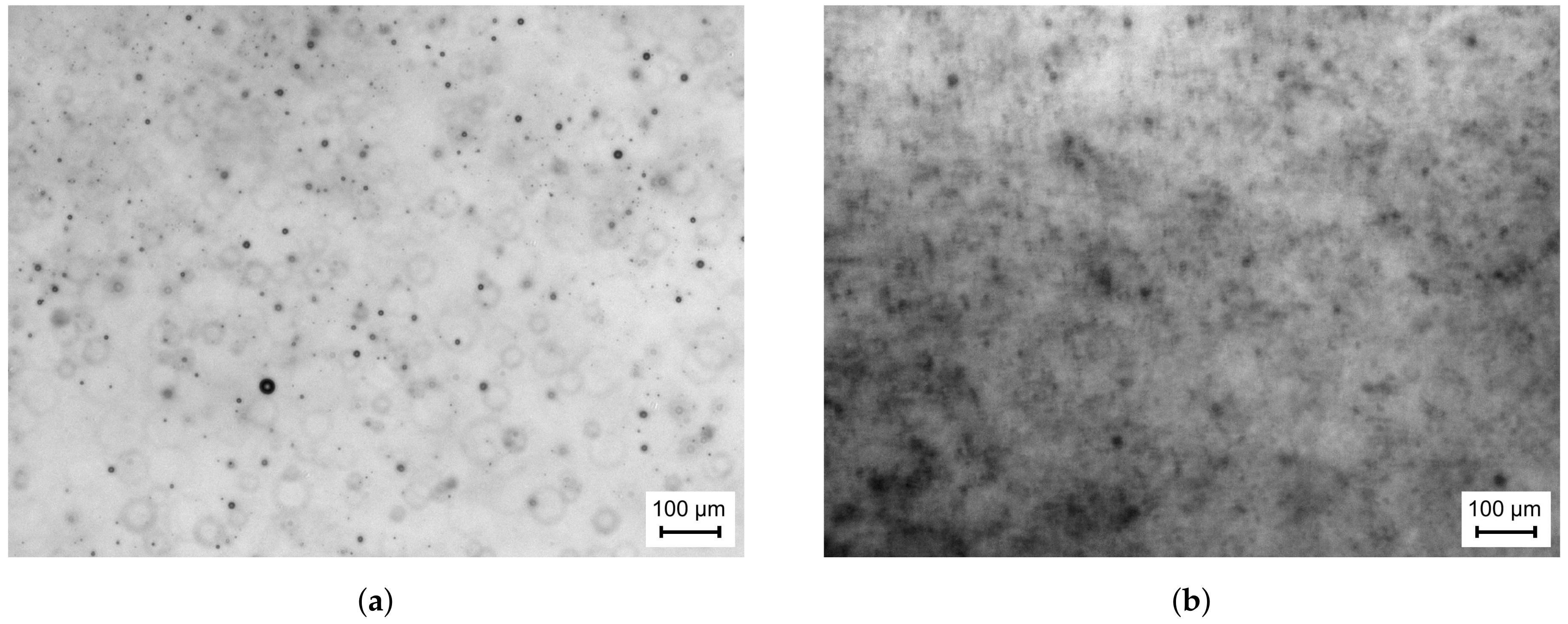
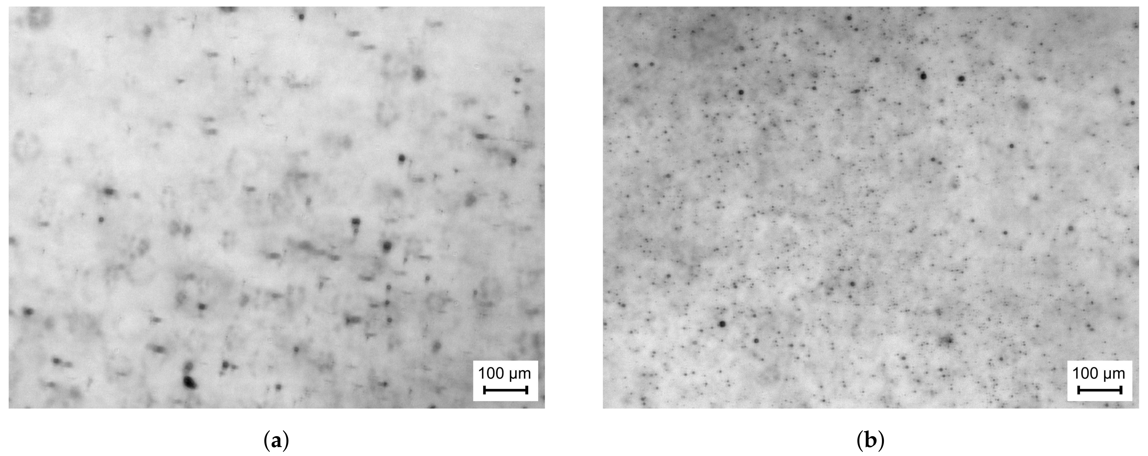
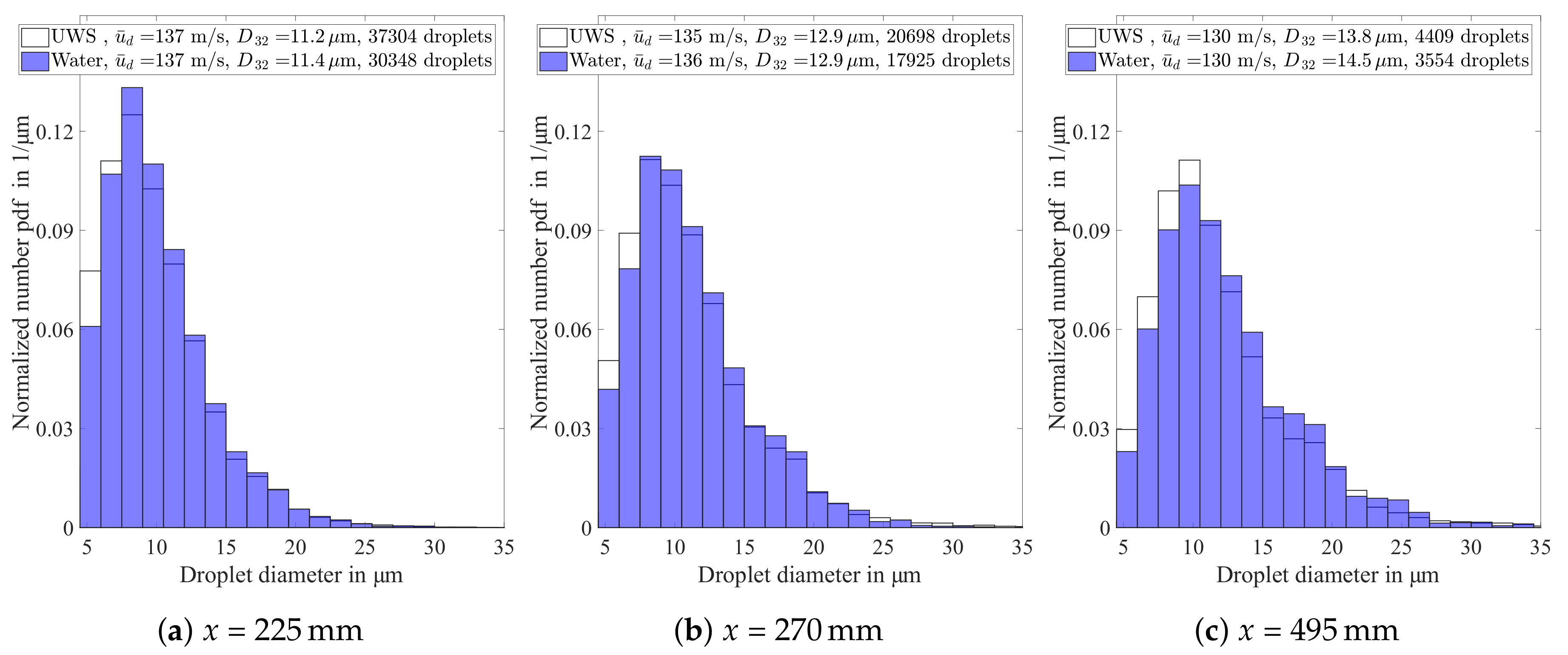
The measured droplet size distribution for UWS and water at the centre of the pipe and at a distance of 225 $\mathrm{m}$$\mathrm{m}$ downstream of the atomiser are illustrated in Figure 16a. At first glance, the normalised number probability density function (PDF) is very similar for both fluids, which confirms the statement that the atomisation process is basically identical. Additionally, the average droplet velocity ${\overline{u}}_{\mathrm{d}}$ of the spray is basically identical. Nevertheless, a detailed comparison reveals a higher probability of small droplets for UWS, whereas most larger diameter classes are characterised by a higher probability of droplets for water. Furthermore, this characteristic effect becomes more prominent with increasing distance from the atomiser as shown in Figure 16b,c. The reason for this phenomenon can be explained by the effect of urea on the evaporation process.

For a further in depth analysis of the evaporation process, the difference between pure water and UWS will be briefly described. First, it is assumed that the Biot number

$$\begin{array}{c}\hfill Bi=\frac{\alpha D_d}{2{\lambda }_d}\ll 1,\end{array}$$

(17)

resulting in uniform temperature within the droplet. According to a Rapid Mixing evaporation model, uniform urea concentration inside the droplet is additionally assumed. With this assumption, the evaporation of an UWS droplet can be subdivided into two stages: The first stage is characterised by an almost exclusive evaporation of water. This means that there will be no evident difference between the evaporation of pure water and UWS. Once the water of the UWS droplet is consumed by evaporation, the evaporation and thermolysis of urea starts. This is the second stage, which can be described as an evaporation process with a considerably lower evaporation rate in comparison to water. Details of modelling the evaporation of UWS are discussed in the work of Birkhold et al. [49].

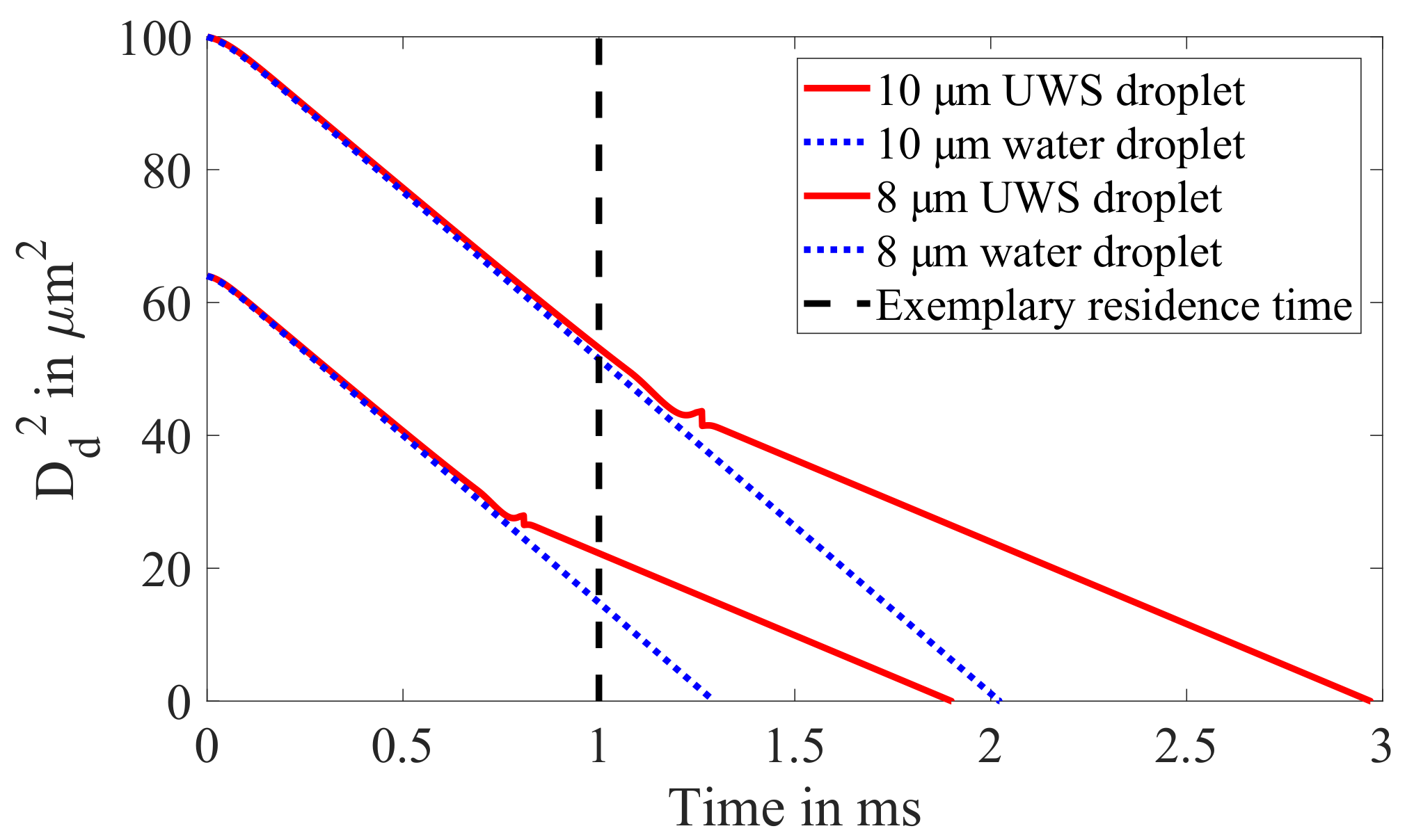
The evaporation process of UWS and water droplets is illustrated in Figure 17 by means of model results for the present hot gas operating condition. Comparing two droplets after an exemplary residence time (dashed line) in the hot gas environment, the 10 $\mathsf{\mu }$$\mathrm{m}$ droplet still behaves like a regular water droplet, whereas the 8 $\mathsf{\mu }$$\mathrm{m}$ features a considerably lower evaporation rate in comparison to water. The important conclusion from the discussion of the evaporation characteristics is that a designated droplet size exists during the lifetime of each UWS droplet, at which the water is completely consumed, and the evaporation rate is drastically reduced.

This knowledge can be transferred to the discussion of the PDFs in Figure 16a–c. The difference in the PDFs between UWS and water is caused by the sudden change of the evaporation rate. In other words, all droplets smaller than a certain size undergo urea evaporation and the thermolysis process, which explains the higher number of UWS droplets in the small diameter classes in comparison to water. The higher probability of all larger diameter classes for the water spray is a consequence of the normalization of the PDF by the total number of droplets. The discussed difference of the PDFs grows stronger with increasing distance from the atomiser, since the residence time of the droplets in the hot gas increases. This results in a progress of spray evaporation and consequently larger droplets will undergo urea evaporation and thermolysis.

In summary, the analysis of the evaporation characteristics reveals promising results, which can be used to study evaporating urea–water sprays. Therefore, the diagnostics may be used to provide validation data for numerical predictions that focus on the evaporation behaviour of UWS. Most importantly, the reasonable and very detailed differences in the droplet diameter distribution emphasize the accuracy of the present spray diagnostics.

4. Conclusions

In this study, a microscopic imaging technique has been developed for recording quantitative spray data in challenging operating conditions. Challenges arise in particular from the high temperatures of the gas phase, which may cause Schlieren effects in the optical path and an astigmatism phenomenon. Both effects did strongly compromise the image quality. As a countermeasure, the optical setup was equipped by a water-cooled window and an astigmatism correction device. By means of an advanced post-processing routine, it is possible to detect droplets as small as 4 $\mathsf{\mu }$$\mathrm{m}$ and droplet velocities up to 250 $\mathrm{m}{\mathrm{s}}^{-1}$ at operating conditions of the gaseous phase of up to 873 $\mathrm{K}$ and $0.6$ $\mathrm{M}$$\mathrm{Pa}$.

Moreover, the traversing of the camera in the direction of the optical axis in a dense spray region turns out to be a great asset. This gives the opportunity to detect inhomogeneous diameter and velocity profiles across the spray cone at a distance of 50 $\mathrm{m}$$\mathrm{m}$ from the atomiser. Hence, valuable droplet data are captured, which may serve as initial conditions for numerical simulations.

Evaluation of the data revealed that the mean gas velocity can be derived from the velocity of the smallest detectable droplets with reasonable accuracy. This gas velocity may be utilised to calculate the temporal mean slip velocity between individual droplets and the gas phase. Hence, the effect of this average slip velocity on secondary atomisation or evaporation can be taken into account. Additionally, the evaluation of the droplet velocity fluctuations in a radial direction reveals vital information about the turbulence of the gas phase, which may be used for validation of numerical predictions. Most importantly, the turbulent dispersion of droplets can be directly evaluated.

In addition to UWS, distilled water was also used as a liquid under otherwise identical conditions. The direct comparison of the droplet diameter distribution between UWS and water revealed typical features of the evaporation characteristics of UWS for all positions downstream of the atomiser.

In summary, the present methodology provides detailed spray data, which can be used to study the evaporation characteristics of UWS under challenging flow conditions. Future work will be focused on the variation of hot gas temperature, pressure and velocity, covering a range of technically relevant operating conditions.