Abstract
The characteristics of series-flow between two consecutive tunnels with distance ranging from 20 m to 250 m are explored by computational fluid dynamics (CFD) parametric simulations of structure and operation parameters. The research indicates that series-flow can be considered the three-dimensional wall jet diffusion of upstream tunnel pollutants under the effects of the negative pressure area of the downstream tunnel entrance. The jet characteristics are primarily related to the tunnel distance between upstream and downstream tunnels and hydraulic diameters, and only influenced by the negative pressure in the area very close to downstream entrance where the tunnel air velocity ratio, i.e., the velocity of upstream tunnel air divided by the velocity of downstream tunnel air, decides the degree of the influence. If ignoring the effects of ambient wind and traffic flow, the series-flow ratio decreases with the increasing of parameters of the normalized tunnel distance, i.e., the tunnel distance divided by tunnel hydraulic diameter, and the tunnel air velocity ratio. Based on the three-dimensional wall jet theory, a series-flow model covering all jet characteristic sections is built. The experiment results indicate that the model applies to consecutive tunnels with any spacing and exhibits higher prediction accuracy.
1. Introduction
With the booming of economy and increasing demand of transportation, more and more tunnels are built to relieve traffic pressure [1,2,3]. A tunnel is a special semi-closed section of road, often with long and narrow structure which makes it difficult to diffuse the exhaust gas (such as CO, NOx) and particles raised by moving cars, seriously degenerating the traffic environment and harming human health [4,5,6,7]. In order to improve the air quality and the safety and comfort of passengers and workers inside the tunnel, longitudinal ventilation, which includes jet fans and vehicle piston wind, is often used, to exchange the air inside and outside the tunnel [8,9] so as to dilute pollutants and discharge them from the tunnel exit. However, for two tunnels nearby, the exhaust gas discharged out from one tunnel can enter the other by circulating wind if the two tunnels are side by side, or by series-flow [10,11] if they are consecutive. That will cause secondary pollution and increase the cost of tunnel ventilation.
There have been many studies made for the recirculating air between laterally adjacent tunnels [12,13,14,15], but still few for series-flow so far. Xiao et al. analyzed the series-flow characteristics of pollutants between two consecutive tunnels with a spacing of 100 m [16], by use of a 1/30 scale model. The results showed when only the upstream tunnel jet fan is started, the series-flow ratio of pollutants is irrelevant to the air velocity of the upstream tunnel exit jet and the concentration of pollutants. Xu Pai et al. [17] used computational fluid dynamics (CFD) technology to study the effects of the tunnel distance within 100 m and the air velocity on series-flow. They concluded that increasing the tunnel distance or the air velocity of upstream tunnel or lowering the air velocity of downstream tunnel, results in an alleviated series-flow. With a 1/30 scale model, Tao et al. [18] studied the relationship between series-flow ratio of consecutive tunnels, where the model tunnel distance was set 3 m, 2.3 m, and 1.7 m. They found that the airflow velocity ratio of upstream and downstream is the key to affect series-flow, and while the change of traffic speed affects series-flow ratio in a limited way the traffic jam does significantly. It should be noted that, with two consecutive tunnels, it requires the tunnel distance in between not to be more than 250 m [19], and the series-flow is essentially the result of interaction between the three-dimensional wall jet of the upstream tunnel exit and the air flow sink of the downstream tunnel entrance. In existing studies, there is a lack of not only systematic analysis on the jet development characteristics of two consecutive tunnels, but also works for the series-flow between two consecutive tunnels with a distance greater than 100 m.
In this paper, series-flow between consecutive tunnels with a tunnel distance ranging from 20 m to 250 m was simulated using CFD at different operation wind speeds. The characteristics of the flow field structure and the change rule of the series-flow ratio were analyzed. A series-flow model was built on basis of the three-dimensional wall jet theory to support environment-friendly ventilation design and economical operation of the consecutive tunnels.
2. Mathematical Model
2.1. Governing Equations
The aim of the research is to reveal the innate law of flow field between consecutive tunnel portals. So in this paper, the influence of both natural wind and traffic wind on air motion and pollutant dispersion between tunnel portals were ignored, and the airflow temperature at all inlet and outlet boundaries was assumed to be 300 K.
The airflow between consecutive tunnels portals can be seen as a steady turbulent flow of incompressible fluid [15]. The Reynolds time-averaged equations (i.e., RANS equations) [20] were used to describe the turbulent flow. Since RANS equations are highly non-linear, with more independent variables than the dimensions of the system, the Standard k-ε turbulence model was used to close the equation system. Its expression is as follows:
where both i and j range from 1 to 3 independently; x stands for the space coordinates; k, ε, ρ, u, and μ are the turbulent kinetic energy, turbulent dissipation rate, air mass density, air velocity, and dynamic viscosity coefficient, respectively; μt = ρCμk2/ε, is turbulent viscosity; the model coefficients Cμ, σk, σε, C1ε and C2ε are 0.09, 1.0, 1.3, 1.44 and 1.92 respectively [21]; Gk refers to the turbulent kinetic energy caused by the average velocity gradient, its expression is:
The species transport equation was used to describe the pollutant dispersion. Considering that the concentrations of pollutant components are scalars and have almost a same normalized distribution. So, CO was used as tracer gas. The species transport equation ignoring buoyancy-driven effects caused by density difference of varied gas components is shown as Equation (4):
where Ss is the production rate, i.e., the mass of s produced by chemical reaction per unit time and volume, Ds and cs represent the diffusion coefficient and volume density of s, respectively. RANS equations and Equations (1), (2) and (4) were the governing equations for the air motion and pollutant dispersion between the consecutive tunnels.
2.2. Computational Geometry, Domain, and Grid
Two-lane and three-lane tunnels with a horseshoe-shaped cross-section were considered and their corresponding hydraulic diameters are, respectively, 6.1 and 8.6 m. In reference to a real tunnel, the tunnel portal’s front slope gradient is 90°. The x-axis is the center line on the tunnel road along the direction from the upstream to downstream. Distance ∆L between upstream and downstream tunnels was set to increase from 20 to 240 m with a step of 20 m. The airflow within a volume of ∆L long, 200 m wide, and 50 m high between the upstream and downstream tunnel portals was simulated. The whole domain was meshed by non-uniform hexahedral grids using ICEM-CFD 17.2 (ICEM-CFD 17.2, ANSYS Inc. Pittsburgh, PA, USA, 2016), and in order to ensure the accuracy and reliability of the calculation, the areas between the upstream outlet and downstream inlet were locally refined.
Figure 1 shows simulation domain and mesh for a three-lane tunnel with ∆L = 60 m, and y coordinate is vertical direction. The number of grids is 2.84 × 10⁶. We conducted numerical simulations with different grid orders of 0.09 × 10⁶, 0.52 × 10⁶, 2.84 × 10⁶, and 6.31 × 10⁶. The result shows that, when the number of grids reaches 2.84 × 10⁶, the simulation results hardly change with the increase of grid number, which means grid independence.
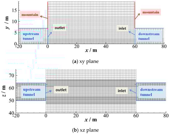
Figure 1.
Simulation domain and mesh for consecutive tunnels.
2.3. Boundary Conditions and Numerical Algorithm
The tunnel walls and pavement as well as the mountain body were taken as an impenetrable, nonslip boundary. Since the Standard k-ε model does not apply to the near-wall area with low Re number, the epsilonWallFunction and kqRwallFunction in OpenFOAM 2.1.1 [22] were assigned to the dissipation rate and turbulence kinetic energy, respectively, to capture the flow structures in near-wall regions.
Due to the application of wall functions, the near-wall node should be located in the log-law regions of a turbulent wall layer instead of the sublayer. That is, the value of y+, as a dimensionless parameter of distance able to describe the flow in the viscous sublayer and log-law layer, should be between 30 and 300. For this study, the thickness of the first layer grid being 0.018 m guaranteed y+ between 33 and 134 under all conditions.
The outer boundary of the computational domain adopted the pressure outlet with gauge pressure being zero. The tunnel inlet and outlet adopted the Dirichlet boundary condition for velocity. According to the possible working conditions of the practical tunnels, the upstream outlet air velocity uup and downstream inlet air velocity udown were all set ranging from 1.5 m·s−1 to 7.5 m·s−1 along the x-direction. The calculations were performed using the OpenFOAM (OpenFOAM 2.1.1, OpenCFD Ltd, Bracknell, UK, 2012), an open source CFD code with an extendable and flexible C++ library.
2.4. Validation
In the experiment of Tao et al. [18], the scale model was composed of two consecutive tunnels and an open roadway section. The radius and length of the single tunnel were set as 0.243 m and 4 m, respectively. The tunnel portals were free of mountains. uup was set 0.75 m·s−1 and uup/udown ranged from 0.47 to 2.58. The numerical model constructed in this paper was used to simulate the airflow and pollutants dispersion between consecutive roadway tunnels, and the structure size of the numerical model is the same as the Tao's tunnel with ∆L = 2.3 m. The comparison of series-flow ratio φs between the simulated and experimental values is made in Figure 2. φs is the series-flow ratio and its expression is φs = Qs/Qup, where Qs stands for the pollutant quantity carried by the series-flow into the downstream tunnel and Qup the total pollutant quantity emitted by the upstream tunnel. It shows that CFD simulated values of series-flow ratio φs are in good agreement with the experimental data, where the maximum error is not more than 8%.
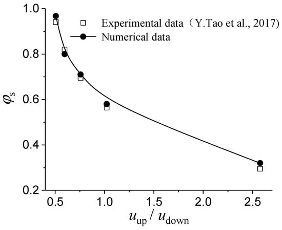
Figure 2.
Impacts of uup/udown on φs.
3. Results and Discussions
3.1. Flow Characteristic
Figure 3 depicts the flow structure at the portals of the three-lane (D = 8.6 m) tunnels under uup = udown = 3 m·s−1. It can be seen that after pollutants are discharged from upstream tunnel exit, they continuously entrain surrounding air and flow downstream, resulting in a spreading jet boundary with increased air flux and lowered velocity. When they arrive at the downstream entrance, pollutants near the tunnel entrance will directly run into the downstream tunnel to form series-flow due to the jet inertia and suction of downstream tunnel entrance. The rest pollutants spread to the upward and two lateral sides of the downstream tunnel entrance due to pressure gradient.
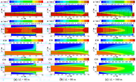
Figure 3.
Flow structure and CO concentration distribution between the portals of consecutive tunnels under different ∆L.
Due to the Coanda effect, the jet flow near the road surface at the entrance is unable to suck air, resulting in a high airflow velocity and low static pressure, in contrast with the upper part of the jet flow where the airflow velocity is small and static pressure is large. The pressure difference between the upper and lower parts makes the jet flow axis close to the road surface, so the influence of the inner layer can be ignored. Assume that the bottom layer thickness of the boundary is 0, so the axis of jet flow coincides with the x-axis; namely the maximum velocity umax of jet flows is always on the x-axis.
According to the attenuation law of umax, the three-dimensional wall jet can be divided into the potential core region and decay region. In the potential core region (where ∆L/D ≤ 7), the umax remains constant, umax/uup = 1; in the decay region (where ∆L/D > 7), with further development of the jet-flow entrainment and mixing of fresh air, the umax begins to decrease [23].
Figure 4 shows the distribution of the maximum flow velocity umax in the symmetric plane of upstream exit jet for different values of ∆L. It can be seen from the figure, whether the downstream tunnel entrance is within the potential core region or the decay region, the change rule of umax of the upstream tunnel exit jet basically matches that of three-dimensional wall jet. Only near the downstream tunnel entrance is umax surged by the negative pressure to deviate from the umax attenuation curve of three-dimensional wall jet.
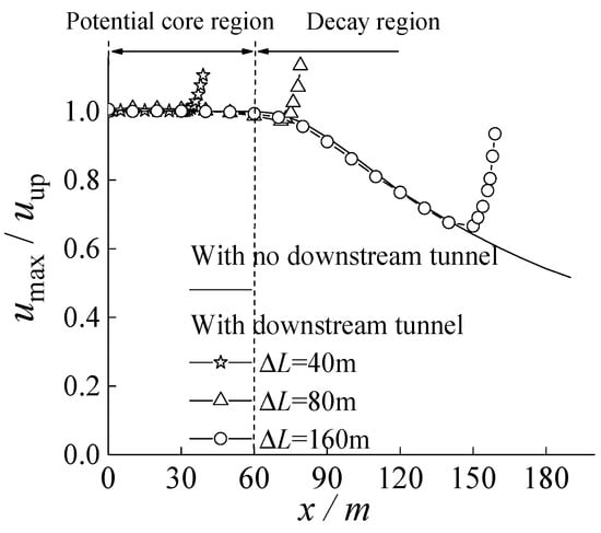
Figure 4.
Distribution of umax in the symmetric plane of upstream exit jet for different values of ∆L.
Figure 5 shows the flow field structure of the three-lane tunnel for ∆L = 120 m with uup/udown being 2, 0.67, and 0.4, respectively, and Figure 6 the change rule of the maximum flow velocity umax in the symmetric plane of upstream exit jet at different values of uup/udown. Based on Figure 5 and Figure 6, one can conclude that the effect of the negative pressure on the upstream jet structure almost has no connection with uup or udown individually but is clearly related to uup/udown. An increased uup/udown will widen the suction range of the downstream tunnel, damage the jet structure of the upstream tunnel exit more obviously, and raise the umax near the downstream tunnel entrance.
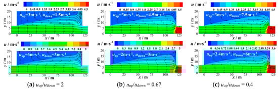
Figure 5.
Series-flow structure for different values of uup/udown.
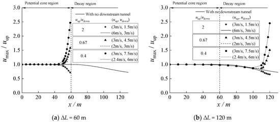
Figure 6.
Distribution of umax in the symmetric plane of upstream exit jet for different values of udown.
Therefore, the series-flow can be considered as three-dimensional wall jet diffusion of the upstream tunnel pollutants influenced by the negative pressure near the downstream tunnel entrance. Jet characteristics are mainly related to ∆L and D. The effect of the negative pressure is confined within the area very close to the downstream tunnel entrance and uup/udown decides its degree.
3.2. Variation Characteristics of the Series-Flow Ratio
The series-flow ratio φs is affected by tunnel operation parameters (i.e., uup and udown) and tunnel structure parameters (i.e., ∆L and D).
Figure 7 shows the relationship between φs and ∆L/D for the tunnels of two lanes (D = 6.1 m) and three lanes (D = 8.6 m), where uup = udown = 1.5 m·s−1. It can be seen that φs decreases with increasing ∆L/D. Figure 8 gives, at uup = udown = 1.5 m·s−1, the longitudinal sections of CO concentration field of three-lane tunnels at different values of ∆L/D (CO concentration is non-dimensionalized). It shows that for a larger value of ∆L/D, the jet is more fully developed with a larger boundary at the downstream tunnel entrance. Thereby, more pollutants are scattered into ambient atmosphere; namely, consistent with Figure 7, φs is smaller.
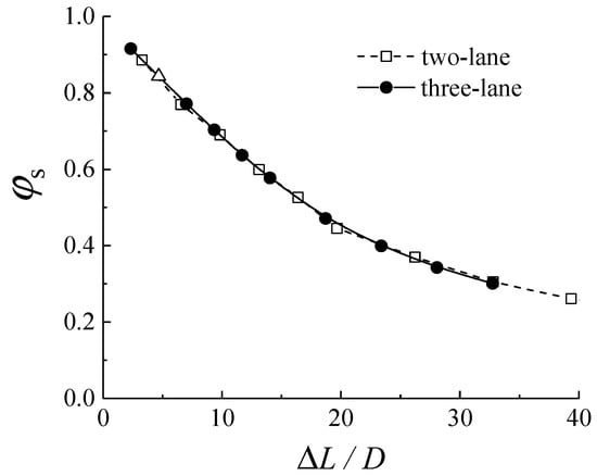
Figure 7.
Impacts of ∆L/D on series-flow ratio φs.
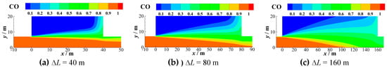
Figure 8.
Distribution of CO concentration in the longitudinal section at different ∆L/D.
Studies have indicated that while φs almost has no connection with uup or udown individually, it is clearly related to uup/udown [18]. Figure 9 shows how φs varies with uup/udown for the tunnels of three lanes (D = 8.6 m) at different values of ∆L/D. At a constant ∆L/D, φs assumes a slowing decrease with the increase of uup/udown. If comparing the results of this paper and Xu‘s model [17], one can see that while φs has the similar change rules in the studies, the difference between them grows up with increasing ∆L/D at a same uup/udown. For example, at ∆L/D = 23.4, the maximum deviation of interflow value between this paper and literature is 53.7%. Xu’s series-flow model can predict the change rules of φs well for ∆L/D < 11.6, but its applicability for ∆L/D > 11.6 needs further verification.
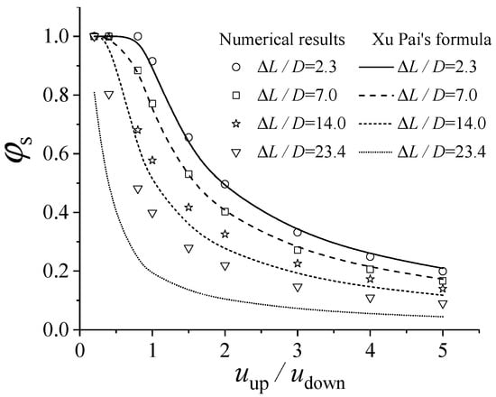
Figure 9.
Impacts of uup/udown on series-flow ratio φs.
3.3. Construction of Series-Flow Ratio Model
Observing the above results of simulations, we construct a model by assuming that φs is mainly influenced by ∆L/D and uup/udown. Noting the jet characteristic that the airflow velocity distribution on the jet cross-section is mainly affected by ∆L/D and only influenced by the negative pressure in the area very close to downstream entrance where uup/udown decides the degree of the influence, the functions of both ∆L/D and uup/udown on the series-flow ratio φs are mutually independent. Therefore, the series-flow ratio model can be written as follows:
The main part of the flow between tunnel portals with different ∆L can be simplified as a form primarily decided by the jet characteristic of the upstream tunnel. And according to the jet characteristic of the upstream tunnel [23], f1(∆L/D) can be constructed in sections.
When ∆L/D ≤ 7, the downstream tunnel inlet is located at the potential core region of the upstream tunnel jet flow. φs is linearly dependent on ∆L/D at uup/udown = 1 (Figure 7). The relation between φs and ∆L/D is fitted as follows by using the simulation results of different ∆L/D and uup/udown = 1 (R2 = 0.995):
When ∆L/D > 7, the downstream tunnel inlet is located at the decay region of the upstream tunnel jet flow. Through surface integration of pollutant concentration and velocity near the downstream tunnel inlet, Qs can be expressed as follows:
where S (m2) is the cross-section area of downstream tunnel entrance and ds is the surface element at any point p on S; r (m) is the distance between p and the x-axis; ur (m·s−1) is the velocity in the x direction at p; cr (ppm) is the pollutant concentration at p. According to three-dimensional wall jet theory [24], expressions of ur and cr are as follows:
In the formula, δ (m) stands for the jet boundary radius at x = ∆L [21], its expression is δ = 1.157D + 0.272∆L; cmax (ppm) is the maximum pollutant concentration of the decay region. Expressions of umax and cmax are as follows:
where cup (ppm) is the initial discharge concentration of the upstream tunnel exit; k is the velocity coefficient; n is the decay index.
Simplifying the tunnel portal into a semicircle of radius R and substituting Equations (8) and (9) into Equation (7) obtain:
In the formula, m = 1 − 1.714(R/δ)1.5 + 1.2(R/δ)3 − 0.308(R/δ)4.5. By substituting jet boundary radius δ and hydraulic diameter D into m, one can obtain m = 1 − 8.944(4.254 + ∆L/D)−1.5 + 32.68(4.254 + ∆L/D)−3 − 43.76(4.254 + ∆L/D)−4.5 ≈ 1 − 8.944(4.254 + ∆L/D)−1.5, noting the absolute value of the omitted part is far less than the remaining part for ∆L/D > 7. Substituting m into Equation (12) obtains:
where ϕx = umaxcmax refers to the maximum flux of pollutant quantity on the jet cross-section, and the second term in the formula of m, 8.944(4.254 + ∆L/D)−1.5, which represents the heterogeneity of the flux distribution of pollutant, gradually fades out as ∆L increases while the pollutant diffusing makes the flux on the jet cross-section more and more uniform.
Combing Equations (6), (10), (11), and (13), φs can be calculated as:
Using the simulation results of different values of ∆L/D and uup/udown = 1, the least square fitted values of k and n are 2.228 and 0.335, respectively, with the goodness of fit R2 = 0.992.
Combining Equations (6) and (14), f1(∆L/D) can be obtained as follows:
With Equation (15), the least square fitting by use of the simulation results of different uup/udown gives f2(uup/udown) = (uup/udown)−0.88, R2 = 0.988. Consequently, the series-flow model can be expressed as:
Figure 10 shows the comparison between prediction results of series-flow model and CFD simulation data. As can be seen, Equation (16) accurately describes the influence of ∆L/D and uup/udown on φs.
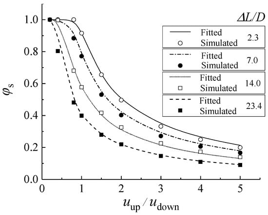
Figure 10.
Comparison of calculated φs with simulated results.
3.4. Validation
Two consecutive tunnels were selected for field measurement of series-flow effect on a windless day, and no vehicles entered the tunnel with the assistance of the local Traffic Management Bureau. Table 1 shows the structural parameters of these tunnels. The ∆L/D values of #1 tunnel and #2 tunnel are 5.9 and 12.6, respectively, representing that the inlets of the downstream tunnels are in the potential core region and decay region, respectively.

Table 1.
Test condition of the consecutive tunnels.
CO2 was used in the test instead of toxic CO. The pollutant-releasing device mainly consist of a vortex flow meter (DN200, CERTEON, Shanghai, China), a CO2 gas canister, and two-stage pressure-reducing valve. In order to ensure its well mixing at outlet section, CO2 was released at 100 m away from the outlet into the upstream tunnel during the test. Figure 11a shows the distribution of CO2 concentration measurement points on the tunnel cross-section. In the figure, H stands for the height of the concentration measuring point from the ground while X stands for the half the width of the tunnel bottom. The values of H for #1 tunnel and #2 tunnel are 0.9 m and 1.4 m respectively, and the values of X are 5.1 m and 6.6 m, respectively. CO2 concentration was measured at the measurement points by concentration transmitters (AR8200, SMART, Guangdong, China). The accuracy of the transmitters is ±(30 ppm + 5% readings). Arithmetic mean value of concentration of the tunnel cross-section is calculated with these measurement points. All the sensors have been calibrated.
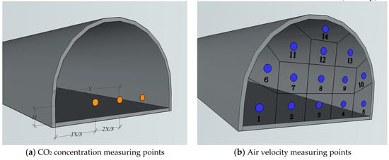
Figure 11.
Arrangement of measuring points.
The jet fans in the tunnels were adjusted to get various values of uup and udown. Figure 11b shows the distribution of 14 air velocity measurement points on the tunnel cross-section. A Testo 425 thermal anemometer (Testo AG, Baden-Württemberg, Germany) was used to measure the air velocity. The accuracy of the anemometer is ±(0.03 m/s ± 5%readings). The mean air velocity of the tunnel cross-section was calculated as an area-weighted value as , where ui is the air velocity at the measuring point within the region i of area ΔSi, and S is the total area of the tunnel entrance.
In each case, the test procedure is as follows: (1) First, adjust the speed of jet fan to change the air velocity inside the tunnel; (2) Second, wait a few minutes to ensure that the speed of airflow in the tunnel is stable. (3) Then, release CO2 and wait for another minute or so to make the concentration of CO2 no longer change significantly; (4) Finally, collect the concentration (velocity) data for one minute and take the mean value of the data as the measured concentration (velocity).
The series-flow ratio φs can be calculated by using the measured air velocity and CO2 concentration, the formula is as follows:
where cup and cdown refers to CO2 concentration of the cross-section in the upstream tunnel and downstream tunnel, respectively; uup and udown is the measured mean air velocity of the upstream tunnel and downstream tunnel, respectively; c0 stands for the local concentration of CO2.
φs under different uup/udown were also calculated by using the model established in this paper as well as the formula given in the existing literature [17,18]. The comparison results are shown in Figure 12. The prediction results of each theoretical model are consistent with the trend of measured data, i.e., φs gradually decreases with the increasing of uup/udown. For #1 tunnel with ∆L/D = 5.9, as shown in Figure 12a, the predictions of the model of this paper and Xu's model are in good agreement with field measured data within an error of 6%; but the prediction of Tao’s model is generally less than the measured value, and the smaller the uup/udown, the bigger the error. Figure 7 and Figure 9 indicate that, with a same uup/udown, the smaller ∆L/D is, the larger φs will be. Noting Tao’s model was based on the model test of consecutive tunnels with ∆L/D = 5.7, the prediction result of φs is supposed to be larger than the measured data of #1 tunnel, and the reason may be that the mountain at the downstream tunnel inlet was neglected in Tao's model test.
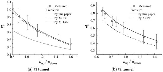
Figure 12.
Comparison of predicted φs with measured results.
For #2 tunnel with ∆L/D = 12.6, as shown in Figure 12b, the deviation between the prediction results of the model of this paper and the measured data is within 5%. However, Xu's prediction value is generally smaller than the measured data, indicating that Xu's model is not suitable for the consecutive roadway tunnels with ∆L/D > 11.6.
4. Conclusions
(1) Series-flow can be considered the three-dimensional wall jet diffusion of upstream tunnel pollutants under the effects of negative pressure of the downstream tunnel entrance. Jet characteristics are mainly related to uup, ∆L, and D. The effects of the negative area on the jet structure are only limited to the area near the downstream opening and udown decides its degree.
(2) Series-flow ratio φs is influenced by tunnel structural and operating parameters. Ignoring ambient wind and traffic flow, φs decreases with increasing ∆L/D and uup/udown.
(3) According to the jet characteristic section of the upstream tunnel where the downstream tunnel entrance is located, a series-flow model covering all jet characteristic sections is built. Beyond the limit of distance between portals from the existing formula, the application scope of series-flow ratio model can be expanded to 0 < ∆L/D < 39.3.
(4) It should be noted that the ambient wind speed and direction, mountain slope at the tunnel entrance, traffic flow states (such as the type and speed of the vehicle), and other external conditions are also important factors to affect the dispersion rules of pollutants between the consecutive tunnels portals. Their effects on series-flow should be studied in future.
Author Contributions
Conceptualization and writing: H.Z. and X.Z.; funding acquisition: K.W. (Ke Wu); supervision: X.Z.; validation: Y.H. and K.W. (Kaijie Wu); writing—original draft preparation: T.Z.; writing—review and editing: K.W. (Ke Wu).
Funding
This research was funded by Natural Science Foundation of Zhejiang province(LY19E080028), National Key R and D Program of China (2017YFC0702504), the Key Research and Development Project of Zhejiang Province (2018C03029), and the Fundamental Research Funds for the Central Universities (2017QNA4023).
Conflicts of Interest
The authors declare no conflict of interest.
References
- Sun, L.W.; Qin, J.S.; Hong, Y.; Wang, L.Z.; Zhao, C.J.; Qin, X. Shield tunnel segment and circumferential joint performance under surface surcharge. J. Zhejiang Univ. 2017, 51, 1509–1518. [Google Scholar] [CrossRef]
- Du, T.; Yang, D.; Peng, S.; Xiao, Y. A method for design of smoke control of urban traffic link tunnel (UTLT) using longitudinal ventilation. Tunn. Undergr. Space Technol. 2015, 48, 35–42. [Google Scholar] [CrossRef]
- Li, J.; Liu, S.; Li, Y.; Chen, C.; Liu, X. Experimental study of smoke spread in titled urban traffic tunnels fires. Procedia Eng. 2012, 45, 690–694. [Google Scholar] [CrossRef][Green Version]
- Bari, S.; Naser, J. Simulation of smoke from a burning vehicle and pollution levels caused by traffic jam in a road tunnel. Tunn. Undergr. Space Technol. 2005, 20, 281–290. [Google Scholar] [CrossRef]
- Bari, S.; Naser, J. Simulation of airflow and pollution levels caused by severe traffic jam in a road tunnel. Tunn. Undergr. Space Technol. 2010, 25, 70–77. [Google Scholar] [CrossRef]
- Raaschou-nielsen, O.; Andersen, Z.J.; Jensen, S.S.; Ketzel, M.; Sorensen, M.; Hansen, J.; Loft, S.; Tjonne, A.; Overvad, K. Traffic air pollution and mortality from cardiovascular disease and all causes: A Danish cohort study. Environ. Health 2012, 11, 60. [Google Scholar] [CrossRef] [PubMed]
- Hoek, G.; Krishnan, R.M.; Beelen, R.; Peters, A.; Ostro, B.; Brunekreef, B.; Kaufman, J.D. Long-term air pollution exposure and cardio-respiratory mortality. Environ. Health 2016, 12, 43. [Google Scholar] [CrossRef] [PubMed]
- Wang, F.; Wang, M.; He, S.; Deng, Y. Computational study of effects of traffic force on the ventilation in highway curved tunnels. Tunn. Undergr. Space Technol. 2011, 26, 481–489. [Google Scholar] [CrossRef]
- Maele, K.V.; Merci, B. Application of RANS and LES field simulations to predict the critical ventilation velocity in longitudinally ventilated horizontal tunnels. Fire Safe. J. 2008, 43, 598–609. [Google Scholar] [CrossRef]
- Lee, H.C.; Yang, C.C. Scale model experiment for the ventilated air interference at intermittent tunnels. In Proceedings of the International Conference, Tunnel Safety and Ventilation, Graz, Austria, 8–10 April 2004; pp. 171–178. [Google Scholar]
- Venås, B.; Johansson, K.; Børresen, B.A.; Pedersen, N. LES analysis of dispersion from road tunnel portals. In Proceedings of the The Sixth International Symposium on Computational Wind Engineering (CWE2014), Hamburg, Germany, 8–12 June 2014. [Google Scholar]
- Zhang, X.; Zhang, T.H.; Zhu, K.; Huang, Z.Y.; Wu, K. Numerical research on the mixture mechanism of polluted and fresh air at the staggered tunnel portals. Appl. Sci. 2018, 8, 1365. [Google Scholar] [CrossRef]
- Tan, X.; Chen, W.; Dai, Y.; Wu, G.; Yang, J.; Jia, S.; Yu, H.; Li, F. Experimental research on the mixture mechanism of polluted and fresh air at the portal of small-space road tunnels. Tunn. Undergr. Space Technol. 2015, 50, 118–128. [Google Scholar] [CrossRef]
- Chen, W.; Guo, X.; Cao, C.; Dai, Y.; Wu, G.; Tan, X.; Yang, J.; Jia, S.; Yu, H.; Li, F. Research on interrelationship of exhaust air of highway forked tunnel and countermeasures. Chin. J. Rock Mech. Eng. 2008, 27, 1137–1147. [Google Scholar] [CrossRef]
- Yang, Y.; He, C.; Zeng, Y. Numerical simulation for the pollution effect between portals of twin highway tunnels. Mod. Tunn. Technol. 2009, 46, 94–98. [Google Scholar] [CrossRef]
- Xiao, Y.M.; Pan, X.H.; Zhang, J.P. Model test system design of channeling effects of air pollutants in continuous road tunnels. China J. Highw. Transp. 2015, 28, 90–97. [Google Scholar]
- Xu, P.; Jiang, S.P.; Lin, Z.; Chen, J.Z. Theoretical research on crossflow pollution in short distance and continuous road tunnels. In Proceedings of the 2012 IEEE International Conference on Industrial Engineering and Engineering Management, Hong Kong, China, 10–13 December 2012. [Google Scholar] [CrossRef]
- Tao, Y.; Dong, J.; Pan, X.; Xiao, Y.; Tu, J. Investigation of the channelling effect on pollutants dispersion between adjacent roadway tunnels. Int. J. Environ. Sci. Technol. 2017, 14, 2733–2744. [Google Scholar] [CrossRef]
- Wang, S.F. Research on the classification of highway tunnel and the concept of highway tunnel group. Highway 2009, 2, 10–14. [Google Scholar]
- An, X.; Song, B.; Tian, W.; Ma, C. Design and CFD simulations of a vortex-induced piezoelectric energy converter (VIPEC) for underwater environment. Energies 2018, 11, 330. [Google Scholar] [CrossRef]
- Tabatabaian, M. CFD module: Turbulent flow modeling. Mercury Learn. Inform. 2015, 43. [Google Scholar]
- Hong, S.W.; Exadaktylos, V.; Lee, I.B.; Amon, T.; Youssef, A.; Norton, T.; Berckmans, D. Validation of an open source CFD code to simulate natural ventilation for agricultural buildings. Comput. Electron. Agric. 2017, 13, 80–91. [Google Scholar] [CrossRef]
- Agelin-Chaab, M.; Tachie, M.F. Characteristics of turbulent three-dimensional wall jets. J. Fluids Eng. 2011, 133, 21201. [Google Scholar] [CrossRef]
- Lu, Y.Q. Heating and Ventilation Design Manual; China Building Industry Press: Peking, China, 1987; pp. 649–651. [Google Scholar]
© 2019 by the authors. Licensee MDPI, Basel, Switzerland. This article is an open access article distributed under the terms and conditions of the Creative Commons Attribution (CC BY) license (http://creativecommons.org/licenses/by/4.0/).