A Sequential Approach to Numerical Simulations of Solidification with Domain and Time Decomposition

Abstract

Progress in computational methods has been stimulated by the widespread availability of cheap computational power leading to the improved precision and efficiency of simulation software. Simulation tools become indispensable tools for engineers who are interested in attacking increasingly larger problems or are interested in searching larger phase space of process and system variables to find the optimal design. In this paper, we show and introduce a new approach to a computational method that involves mixed time stepping scheme and allows to decrease computational cost. Implementation of our algorithm does not require a parallel computing environment. Our strategy splits domains of a dynamically changing physical phenomena and allows to adjust the numerical model to various sub-domains. We are the first (to our best knowledge) to show that it is possible to use a mixed time partitioning method with various combination of schemes during binary alloys solidification. In particular, we use a fixed time step in one domain, and look for much larger time steps in other domains, while maintaining high accuracy. Our method is independent of a number of domains considered, comparing to traditional methods where only two domains were considered. Mixed time partitioning methods are of high importance here, because of natural separation of domain types. Typically all important physical phenomena occur in the casting and are of high computational cost, while in the mold domains less dynamic processes are observed and consequently larger time step can be chosen. Finally, we performed series of numerical experiments and demonstrate that our approach allows reducing computational time by more than three times without losing the significant precision of results and without parallel computing.

1. Introduction

Modeling and computer simulation become very effective tools in studying difficult problems in foundry and metallurgical manufacturing. Computational investigations provide insight into the process that otherwise would be very difficult to obtain. For example, acquiring the complete temperature field evolution for a given casting is almost an elementary step in computational studies, but it experimentally requires sophisticated tools to visualize the entire temperature field. Moreover, computational studies are of high importance when there is a need to optimize casting production. Typical trial and error approaches are very often insufficient and, more importantly, can be very laborious and expensive. Especially, when significant changes in the protocol need to be tested (e.g., several molds, miscellaneous material properties or initial setups). Using modeling tools, even a large series of studies can be performed without significant changes in the working space. Moreover, they allow investigating the sensitivity of the given casts to changes in materials parameters or processing conditions.

However, in order to effectively perform a large series of computational studies using reasonable resources, the framework needs to be not only accurate but also computationally efficient. Combinatorial studies of phase space involve a large number of individual simulations. Moreover, increasing precision of simulation typically leads to larger individual computational problems that need to be solved. In both cases, improving computational efficiency, while providing high accuracy, is of utmost importance, with several remedies already available. For instance, one option is to harness large computing clusters either based on CPUs or accelerated architectures such as GPUs [1,2,3,4,5].

However, these require at least minimal expertise in high-performance computing, although they are feasible, they may not be easily available. Another option is to explore more advanced computational techniques (e.g., hp-adaptation, parallel computing) that minimize computational cost while providing an accurate solution.

In this work, we discuss a technique called mixed time partitioning, where a considered structure is divided into sub-domains modeled by various procedures [6].

This approach fits typical characteristics of solidification, where physical processes inside mold are significantly different from those in a solidifying casting. Processes occurring in casting are more dynamic, and they require a more accurate solution, i.e., small time step. On the other hand, a heat transfer within mold sub-domain is less intense, and thus coarse-grained step is sufficient to guarantee the desired precision of computations. As a result, different time steps can be chosen for individual sub-domains and significant saving can be achieved. However, the choice of multiplication factor (a quotient time step in mold and time step in casting) is crucial for the accuracy. We discuss the detailed algorithm and the results of numerical simulations obtained by its use. We showcase that the mixed time partitioning method improve computational efficiency and gives promising results for future work.

Casting is one of the common techniques to fabricate metal machine elements and tools. Properties of final casting products depend on the interplay between many physical processes involved. Typically there is a complex interplay between various phenomena, such as liquid-solid phase transformation, heat transfer including latent heat generation, solute diffusion, fluid dynamics, and mold filling, just to name few [7,8,9,10,11,12,13].

Understanding, the interaction between these, provides a rationale for casts design of desired properties. Computational techniques afford very odd ways to study these systems.

The problem of adequate modeling of foundry systems depends on the solution of heat transfer described by a partial differential equation. In simple cases, the equation can be analytically integrated with respect to space and time to yield accurate solution (see Figure 1).

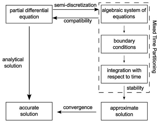
Figure 1. Transition from partial differential equation to approximate solution by using mixed time partitioning methods.

However, because of a complicated phenomenon, such as solidification, it is impossible to carry out a corresponding analytical solution directly. In this case, it is necessary to perform numerical calculations. In particular, we study the temporal and spatial evolution of the temperature field in the casting. In such case, the precision of computations is affected by two main factors: domain decomposition—so-called semi-discretization (i.e., size and type of a finite element) and time discretization (i.e., size of a time step). In this work, we focus on the time discretization—so-called time decomposition to different sub-domains. We explore improvement in computational efficiency of time steppers by studying a combination of different time integration schemes used in various sub-domains. We develop an approach, that is a generalization of two other techniques, namely sub-cycling methods and partitioning integration methods [8,11,13] (see Figure 2).

Figure 2. Origin of mixed time partitionig methods.

Such combination allows to better estimate the size of time step and time integration scheme for the problem of interest.

2. Numerical Model of Solidification

Solidification is described by a quasi-linear heat conduction equation with additional heat source term along with the boundary and initial conditions:

$$\nabla ·(\lambda \nabla T)+{\rho }_{s}L\frac{\partial f_s}{\partial t}=c\rho \frac{\partial T}{\partial t},$$

(1)

$${\mathsf{\Gamma }}_1:q=\alpha \left(T\right)(T_{|{\mathsf{\Gamma }}_1}-T_{env}\left(t\right)),$$

(2)

$${\mathsf{\Gamma }}_2:\left\{\begin{array}{l}{\displaystyle -{\lambda }_1\frac{\partial T^{\left(1\right)}}{\partial \mathbf{n}}=-{\lambda }_2\frac{\partial T^{\left(2\right)}}{\partial \mathbf{n}}=\frac{\beta }{\delta }(T^{\left(1\right)}-T^{\left(2\right)}),}\\ T^{\left(1\right)}\ne T^{\left(2\right)},\end{array}\right.$$

(3)

where $\lambda$ is the thermal conductivity coefficient, c is the specific heat, $\rho$ is the density (subscript s refers to the solid phase), L is the latent heat of solidification, $f_s$ is the solid phase fraction, q is the heat flux, t is the time and T is the temperature. Boundary condition given by Equation (2) is the Newton boundary condition, where the exchange of heat on ${\mathsf{\Gamma }}_1$ with the environment takes place with heat transfer coefficient $\alpha$. $T_{|{\mathsf{\Gamma }}_1}$ is the temperature on the ${\mathsf{\Gamma }}_1$ boundary of the domain and $T_{env}$ is the environment temperature. Boundary condition given by Equation (3) is the continuity boundary condition on the ${\mathsf{\Gamma }}_2$ boundary separating ${\mathsf{\Omega }}_1$ and ${\mathsf{\Omega }}_2$ domains with temperature $T^{\left(1\right)}$ and $T^{\left(2\right)}$, respectively. The thermal conductivity coefficient of the material in the separating layer is given by $\beta$, and $\delta$ is the thickness of this layer and $\mathbf{n}$ is the normal vector to the boundary.

In this work, we use the apparent heat capacity formulation ($c^{*}$) of solidification:

$${\displaystyle \nabla ·(\lambda \nabla T)=c^{*}\left(T\right)\frac{\partial T}{\partial t},}$$

(4)

$$\begin{array}{lll}{c}^{*}& =& c{\rho }_s,\mathrm{for}T<T_s,\\ c^{*}& =& {\displaystyle c{\rho }_f-{\rho }_{s}L\frac{\partial f_s}{\partial T},\mathrm{for}{T}_s\le T\le T_l,}\\ c^{*}& =& c{\rho }_l,\mathrm{for}T>T_l.\end{array}$$

(5)

where subscript l refers to the liquid phase, $T_s$ is the solidus temperature (the end of solidification) and $T_l$ is the liquids temperature (the beginning of solidification). We used indirect model of solid phase growth for two-component alloy:

$${\displaystyle f_s\left(T\right)=\frac{1}{1-\eta k\epsilon }\left(1-{\left(\frac{T_M-T}{T_M-T_l}\right)}^{\frac{1-\eta k\epsilon }{k-1}}\right),}$$

(6)

where $\eta$ is the coefficient describing the grain’s shape, k is the solute partition coefficient, $T_M$ is the solidification temperature of the pure basic component of an alloy, and $\epsilon$ is the so-called Brody–Flemings coefficient. For more details, we refer to [14,15].

All the above equations form the thermal description basis of solidification. Generally speaking, to solve this initial boundary value problem we first introduce spatial discretization and then time discretization (see Figure 1). Firstly, we use the finite element method ([16,17,18,19,20,21] et al.) to obtain the ordinary differential equation, given as:

$$\mathbf{M}\left(T\right)\dot{\mathbf{T}}+\mathbf{K}\left(T\right)\mathbf{T}=\mathbf{b}\left(T\right),$$

(7)

where $\mathbf{M}$ is the capacity matrix, $\mathbf{K}$ is the conductivity matrix, $\mathbf{T}$ is the temperature vector and $\mathbf{b}$ is the right-hand side vector, whose values are calculated on the boundary conditions basis. Secondly, we apply time steppers to solve ordinary differential equation. This step is the major element of this work. We studied several combinations of various schemes from the family of one step $\mathsf{\Theta }$ time integration schemes [21,22]:

• overall formula of the one step $\mathsf{\Theta }$ schemes

  $$(\mathbf{M}+\mathsf{\Theta }\Delta t\mathbf{K}){\mathbf{T}}^{n+1}=({\mathbf{M}}^n-(1-\mathsf{\Theta })\Delta t{\mathbf{K}}^n){\mathbf{T}}^n+\Delta t{\mathbf{b}}^n,$$

  (8)
• for $\mathsf{\Theta }=0$ it is Euler Forward (conditionally stable) scheme

  $${\mathbf{M}}^n{\mathbf{T}}^{n+1}=({\mathbf{M}}^n-\Delta t{\mathbf{K}}^n){\mathbf{T}}^n+\Delta t{\mathbf{b}}^n,$$

  (9)
• and for $\mathsf{\Theta }=1$ it is modified Euler Backward (unconditionally stable) scheme

  $$\left({\mathbf{M}}^n+\Delta t{\mathbf{K}}^n\right){\mathbf{T}}^{n+1}={\mathbf{M}}^n{\mathbf{T}}^n+\Delta t{\mathbf{b}}^{n+1},$$

  (10)

  where $\Delta t$ is time step and superscript n refers following step of computations.

2.1. Mixed Time Partitioning Methods

In this work, we propose to use a combination of various time stepping schemes either explicit and/or implicit. These are two basic classes of time stepping schemes. Explicit methods usually are less computationally demanding, but small time step is required for numerical stability. Implicit methods, on the other hand, are more computationally expensive with much larger time step allowed and in general with better stability. Enhanced stability of implicit methods is one of the reasons for their widespread use in many engineering problems. However, when the too large time step is used, although numerically stable, implicit methods may give error-ridden solutions. For problems like solidification in casting such errors propagate quickly. Therefore, the choice of time stepping scheme should be based on the computational requirements but also should take into account the nature of modeled phenomena. In problems like the one considered here, with two significantly different natures between sub-domains, it may be beneficial to combine two time stepping schemes for different sub-domains. It is the primary motivation for this work and the basic idea of the mixed time partitioning method. In particular, we use different integration schemes in different parts of modeled domains (E—explicit, I—implicit). Moreover, to improve computational efficiency more significantly we seek to decrease the size of the time step, in sub-domains where it is justified. The choice of size of the time step is based on the numerical stability analysis ($\Delta t<\Delta t_{critic}$), as we showed in [23,24,25].

In Table 1, we summarize the combinations of time integration schemes we investigate.

Table 1. The combination of applied integration schemes. (m is a numerical stability coefficient, $\mathsf{\Theta }$ is a parameter of one-step time integration scheme—assumes value 0 or 1 in the examined case, I is a symbol indicating the implicit scheme, and E a symbol indicating the explicit scheme).

m	${\mathbf{\Theta }}_{\mathit{cast}}$	${\mathbf{\Theta }}_{\mathit{mold}}$${\mathbf{\Theta }}_{\mathit{core}}$	$\mathbf{\Delta }{\mathit{t}}_{\mathit{cast}}$	$\mathbf{\Delta }{\mathit{t}}_{\mathit{mold}}$$\mathbf{\Delta }{\mathit{t}}_{\mathit{core}}$	Symbol of sub- and total-Cycle	Description of Symbols sub- and total-Cycle (Integration Scheme)
≥2	1	1	$\Delta t$	$m\Delta t$	$I-I^m$	Implicit − Implicit
≥2	0	0	$\Delta t$	$m\Delta t$	$E-E^m$	Explicit − Explicit
≥2	0	1	$\Delta t$	$m\Delta t$	$E-I^m$	Explicit − Implicit
≥2	1	0	$\Delta t$	$m\Delta t$	$I-E^m$	Implicit − Explicit

2.1.1. Sub-Cycles and Total-Cycles

The separation of all domains into two groups: (i) a mold and cores (domains with similar properties as mold which help in heat carrying out from the cast) and (ii) a casting, so-called sub-domains, offers the possibility to use different time stepping schemes in every group. Moreover, the mixed time partitioning method allows selecting the size of time steps in various sub-domains of the computational mesh. In particular, firstly a small and fixed time step $\Delta t$ in casting domain B is determined. Then, in mold/cores sub-domain A it is beneficial to choose a time step $m\Delta t$, where m is a stability coefficient which is a positive integer value resulting from stability requirements. The local time step in the given sub-domain is always chosen on the basis of the analysis (necessary conditions are described in [25]).

It is important to note that the stability analysis is local and the stability restriction of one sub-domain does not enforce the size of the time step for the entire mesh.

Using sub-cycles requires that two systems of equations are being constructed: (i) one for casting when only sub-cycles are considered and (ii) one for all domains (mold, core, and casting) when a total cycle is considered. In practice, global matrices and vectors are assembled according to the elements partitioning (see Figure 3). Calculations connected to casting domain are made in sub-cycles with time step $\Delta t$. Temperature vector is being updated only for elements belonging to casting domain. All elements in the mesh take part in calculations made in total-cycles with a time step $m\Delta t$.

Figure 3. Formation of global matrix coefficients in mixed time partitioning methods (block matrix where B refers to cast domain, A refers to other domains).

2.1.2. Determination of Critical Time Step

The stability analysis is one of the main elements of a mixed time partitioning method. It is necessary to clearly define conditions which must be fulfilled in order to ensure numerical stability of the numerical results. More details can be found in [23,25].

Briefly, the stability criterion is determined for i-finite elements based on eigenvalues ${\mu }_i$ of the amplification matrix—capacity and conductivity matrices. The critical time step $\Delta t_{crit}$ in the stability criterion is determined as follows:

$$\Delta t_{crit}\le \frac{2}{{\mu }_i},$$

(11)

where ${\mu }_i=max\left({\mu }_i^{\left(e\right)}\right)$ is the maximum eigenvalue among all elements in the chosen sub-domain (i.e., in the cast). In general, the maximal eigenvalue is problem specific and it depends on the material properties and geometry of the finite elements.

The critical time step is determined for individual sub-domains, and the integer coefficient is computed as follows:

$$m=⌊\frac{\Delta t_{mold}}{\Delta t_{cast}}⌋.$$

(12)

The multiplication factor m includes information about elements and is computed once before starting the simulation (details on [23,25]).

2.1.3. Solution Algorithm

Handling the boundaries between domains is one of the challenges in mixing time partitioning method. To avoid this obstacle, we introduce double numbering of nodes while keeping the same coordinates (Figure 4) see in [15].

Figure 4. Double numbering of nodes (with the same coordinates) belonging to two sub-domains.

Thanks to this extra step we get natural separation of domains with different thermo-physical properties. Additionally, the double indexing helps to reorganize the block matrix in the corresponding system of equations (see Figure 3). Finally, such operations greatly simplify the numerical stability analysis of the chosen method.

The following protocol (Algorithm 1) is used to perform computations related to the casting domain. A counter c controls if total-cycle or sub-cycle is considered, it is defined as:

$$c=s\mathrm{mod}m,s=1,2,\dots ,n_{step}$$

(13)

where $n_{step}$ is the total number of given steps of computations during simulation.

Algorithm 1 Protocol of computations

set beginning conditions, $s\leftarrow 1$, $c\leftarrow 1$ repeat     if $c\ne 0$ then perform computations for sub-cycles:         assembly system of equations for elements in casting domain;         apply boundary conditions for casting domain;         compute temperature vector $T^{n+1}$ for casting domain;     end if     if $c=0$ then perform computations for total-cycles:         assembly system of equations for all elements;         apply boundary conditions for all domains;         compute temperature vector $T^{n+1}$ for all domains;     end if     increase computation step $s\leftarrow s+1$; until $s<n_{step}$;

3. Results and Discussion

We have implemented the mixed time partitioning method in C++ programming language as an extension to the author’s simulation framework called NuscaS [26].

We have used finite element method to solve apparent heat capacity formulation of solidification, given by the Equation (4) supplemented by boundary conditions (Equations (2) and (3)). We used indirect model of solid phase growth for binary alloy (Equation (6)).

We performed a series of numerical simulation of solidification for Al–2%Cu alloy casting solidifying in the metal form (the popular alloy for which there are known thermo-mechanical properties and behavior during solidification and cooling, it used in many foundries). The analyzed casting together with mold and cores are shown in Figure 5. The values of material properties of the liquid phase, solid phase and mold/core are given in Table 2. The physical properties are implicitly included in the algebraic system of equations (Equation (7)).

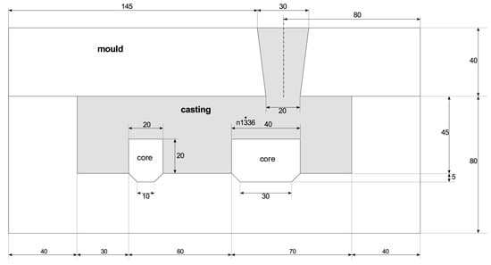
Figure 5. The analyzed casting in mold.

Table 2. Physical properties of cast and mold/core material using during computer simulation of Al–2%Cu alloy solidification.

Quantity	Unit Symbol	Liquid Phase	Solid Phase	Mold/Cores
density	kg/m${}^3$	2498	2824	7500
specific heat	J/kgK	1275	1077	620
thermal conductivity	W/mK	104	262	40

We set the initial temperature of liquid alloy, mold, and core to 960 K 590 K and 540 K, respectively. We considered non-ideal contact between casting and mold (with the conductivity of the separating layer 1000 W/m${}^2$K) and between casting and the core (with conductivity 800 W/m${}^2$K). We applied Neumann boundary conditions on all other boundaries. We set environment temperature as 300 K and heat exchange coefficient as 100 W/m${}^2$K. The time step $\Delta t=0.0035$ s was used in the computer simulations.

Such configuration of initial and boundary conditions along with materials properties allows us to study both solidifying of the cast and subsequent cooling of the entire system. We study temperature evolution and solid phase growth for 450 s. First 145 s corresponds to the solidification. The remaining time corresponds to the solid-state cooling ($f_s=1$ in the entire casting).

We depict the geometry and dimensions of the considered system in Figure 5, and the mesh in Figure 6. The computational mesh consists of 16,261 triangular finite elements with 8640 nodes (only 2125 nodes belongs to the casting domain). In further analysis, we focus on the selected node (n1336) that we denote in Figure 5. That node belongs to several finite elements lying in the central and the longest solidifying part of the casting. This choice is dictated by the possibility to trace the results from the beginning to the end of the slow solidification in the central part of the cast.

Figure 6. Finite element mesh in analyzed system.

Solidification in the castings is a complex phenomenon where the behavior of one part may be significantly different from other part’s behavior. Solidification process may take place at a constant temperature or temperature range. If the solidification occurs at a constant temperature, then it is considered to be the so-called solidification with zero temperature range [27].

However, solidification of most of the alloys (including one considered in this work) occurs in some temperature ranges. It starts at liquidus temperature ($T_l$) and ends at solidus temperature ($T_s$) or at eutectic temperature ($T_E$). The casting is in a liquid state above the liquidus temperature ($f_s=0$). When the temperature decreases below the liquidus temperature, but it is above the solidus temperature, casting begins to solidify, and the solid phase appears ($0<f_s<1$). In this discussion, we take into account indirect solid phase growth model, and therefore casting solidifies in the range from liquidus temperature to reaching of the eutectic temperature. Below the eutectic temperature, for which $f_s=1$, only the cooling process takes place. With reference to the co-occurring phenomena, we take into account the changes in temperature and the solid phase fraction in the discussion of the obtained results. Temperature range is between 960 K and 530 K for figures with temperature field, and solid phase fraction range is between 0 and 1 for figures with the solid phase fraction field.

We use so-called cooling curves to study the temperature changes over time for a selected location in the casting. The solidification process is the most intricate in the central zone of the casting and between the two cores, as here the solidification occurs at the slowest rate. We select the node in this zone (i.e., node 1336) to showcase the thermal behavior and plot in Figure 6. Initially, we see only cooling that is proceeded by the solid phase formation accompanying the latent heat release. After $136.5$ s, we record the end of the solid phase formation with $f_s=1$. After that time, we see only cooling. We plot the corresponding temperature field in Figure 7. Because of the most complex interplay between cooling and solid phase formation in the central zone, we choose this location to perform the verification. In particular, we use cooling curves and the rate of solid phase growth at node 1336 for three time steps (after $65.5$, 75, 95 s).

Figure 7. Temperature field obtained for selected point in casting domain after 136.5 s of solidification process (red color denotes the highest temperature and yellow color denotes the lowest temperature in the cast). Four combination of the time integration schemes (A) $I-I^m$, (B) $E-E^m$, (C) $E-I^m$, (D) $I-E^m$ for multiplication factor $m=1$.

We analyze the computationally efficient of the used mixed time partitioning method. In particular, we focus on answering two main questions. First, we ask how much we can gain by using the mix of various methods for different parts of the computational domain. We study various combinations of methods from two basic families of time steppers (explicit vs. implicit and its combination). Then we ask the question about computational gains due to applying sub-cycles. Finally, we focus on the accuracy of the solution. To the best of the author’s knowledge, this is the first computational study of casting’s solidification that involves mixed time partitioning methods.

3.1. Mixed Time Partitioning Methods vs. Sub-Cycling and Partitioning Methods

We study the total run time required to simulate the solidification and cooling of the casting over 450 s. In our analysis, we consider four cases of numerical simulation:

(i)

traditional methods—when the same time integration schemes and the same time steps are used in each sub-domains (Table 3),

Table 3. A total time t of computations obtained for the traditional methods ($m=1$). The same integration methods and the same time step.

Symbol	Description	t [s]
$I-I^m$	Implicit in cast domain − Implicit in other domains	3841.51
$E-E^m$	Explicit in cast domain − Explicit in other domains	2340.73

(ii)

sub-cycles methods—when the same time integration schemes and the different time steps are used (Table 4),

Table 4. A total time t of computations obtained for the sub-cycles methods ($m=15$). The same integration methods and the different time step.

Symbol	Description	t [s]
$I-I^m$	Implicit in cast domain − Implicit in other domains	1535.98
$E-E^m$	Explicit in cast domain − Explicit in other domains	1225.42

(iii)

partitioning methods—when the different time integration schemes and the same time steps are used (Table 5),

Table 5. A total time t of computations obtained for the partitioning methods ($m=1$). The different integration methods and the same time step.

Symbol	Description	t [s]
$E-I^m$	Explicit in cast domain − Implicit in other domains	3268.53
$I-E^m$	Implicit in cast domain − Explicit in other domains	3557.40

(iv)

mixed time partitioning methods—when the different time integration schemes and the different time steps are used (Table 6).

Table 6. A total time t of computations obtained for the mixed time partitioning methods ($m=15$). The different intergration methods and the different time step.

Symbol	Description	t [s]
$E-I^m$	Explicit in cast domain − Implicit in other domains	1053.95
$I-E^m$	Implicit in cast domain − Explicit in other domains	1539.86

We have gathered data for four cases listed in Table 1. We measured run time includes the assembly of the system, the applying boundary conditions and solving the system of equations. We report $E-E$ combination to be the fastest while $I-I$ to be the slowest case (because of many iterations per one time step). The major difference comes from the protocol the system of equation is assembled and solved. In $I-I^m$ case, both the boundary condition and solving system of equations are iterative processes and require more time to be completed. We note that in the above cases the multiplication factor $m=1$ and the mixed time partitioning methods are very similar to the conventional methods. However, we decided to include these results to establish the baseline for sub-cycles time steppers, which we discuss in the next subsection.

3.1.1. Computational Efficiency of Sub-Cycling Methods

We will discuss the case with the same time integration schemes but with different time steps used in the casting and mold. In this approach, we use a fixed time step $\Delta t$ in the cast domain and much larger time steps $m\Delta t$ in the mold domains. The maximal multiplication factor we study in this paper is $m=15$. It is the largest acceptable value of m chosen based on the numerical stability criterion. This strategy allows accounting for the essential physical features occurring in the casting which are not important in the mold. From Table 4 we can see that, like in the case of a traditional schemes combination, $E-E^m$ methods are faster than the $I-I^m$ ones (long-lasting iterations). A dynamically changing physical phenomena in the casting require very small time step. It is favorable for explicit steppers. Implicit schemes fulfill many iterations per one time step. Therefore, the run time is extended. Despite this fact, the sub-cycling methods are faster than the standard methods (for $m=1$).

3.1.2. Computational Efficiency of Partitioning Methods

In this section, we discuss the case where different time integration schemes are used with the same time step used in both domains: the casting and mold. We consider two cases: (i) explicit time stepper used in the cast domain with implicit time stepper used in the mold domains and (ii) implicit time stepper used in the cast domain with explicit time stepper used in the mold domains. We include the total run times in the Table 5. Our investigations indicate the shortest total run time for $E-I^m$ combination, comparing to the $I-E^m$. The difference in the run times originates from the difference in the way boundary conditions are applied, and the system of equations is solved. The introduction of the natural (contact) boundary condition is carried out by means of elements which are the boundary’s discretization. The introduction of the above boundary condition in implicit time stepper requires modifying the coefficients of matrix and right-hand vector while in explicit time stepper only the coefficients of the right-hand vector. It is the reason for extended a run time when we use implicit schemes in a casting domain.

3.1.3. Computational Efficiency of Mixed Partitioning Methods

We now move to the more complex case in which we test not only various combinations of different time steppers, but also different size of the time step. Intuitively, based on our understanding of the underlying physics, we choose the combination of explicit schemes with the small size of time step in the casting and implicit schemes with coarse-grained time step. From Table 6 we can see that, as in the case of a previous combination of schemes, $E-I^m$ methods are faster than the $I-E^m$ ones. Using explicit schemes in the casting domains give abbreviated run time and a better description of the physical phenomena occurring during casting solidification.

Here, we also study four different combinations of steppers. We include the run time of the given method in Table 7. For the purpose of these tests, we define the efficiency $p_m$ as a ratio between run time t for $m=1$ (the standard approach) and the run time for $m=15$. From the collected data, we see a computational gain for all studied cases considered.

Table 7. An efficiency $p_m$ obtained with the mixed time partitioning methods.

	$\mathit{m}=1$		$\mathit{m}=15$
	$t,s$	$p_m$	$p_m$
$I-I^m$	3841.51	1	2.5
$E-E^m$	2340.73	1	1.9
$E-I^m$	3268.53	1	3.1
$I-E^m$	3557.40	1	2.3

This confirms the efficacy of the mixed time partitioning methods when applied to modeling of solidification process. The largest computational gain is possible when an explicit scheme is used in the casting sub-domain and the implicit scheme in the mold sub-domains. It is the most intuitive combination of time integration schemes for the modeled phenomena of interest. In numerical considerations, the observed gain has origins in the way boundary conditions are applied, and the system of equations is solved. Moreover, the results are obtained with an extensive iterative method when we use implicit methods.

However, the computational gain is not the only criteria. The accuracy of the solution is an equally important criterion which will be discussed in the next subsection.

3.2. Accuracy of the Numerical Solution

Finally, we discuss the accuracy of the proposed method. In particular, we compare the cooling curve for different configurations discussed above. We choose one node in the cast and extract the temporal evolution of two quantities: temperature and the solid phase fraction. We plot both quantities of interest in Figure 8 and Figure 9. We compare four various combinations of time integration schemes for the case $m=1$ (the standard and partitioning methods). We notice only small differences in temperature and solid phase profile between tested cases. All of them appear under the eutectic temperature where the casting is completely solidified, and a cooling process occurs. We observe the largest differences (the highest standard deviation) for the combination of $E-E^m$. However, these differences are small (for $m=15$ even smaller) and do not exceed a few percents, which is acceptable.

Figure 8. Cooling curves obtained for selected point in casting domain. Temperature distribution for multiplication factor $m=1$ calculated by mixed time partitioning methods.

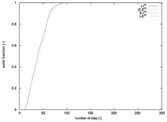
Figure 9. Solid phase growth obtained for selected point in casting domain. Solid phase fraction for multiplication factor $m=1$ calculated by mixed time partitioning methods.

We further test the accuracy of the sub-cycles and mixed time partitioning methods ($m=15$). We plot corresponding profiles of temperature and solid fractions in Figure 10 and Figure 11. The shape of both presented curves indicates that between the liquidus and solidus temperatures solidification process occurs expectedly. Moreover, the distribution of temperature and solid phase fraction obtained for multiplier $m=15$ is consistent with the above observations. The differences appearing between applied schemes are smaller than mentioned above one (for $m=1$). The benefits of using mixed time partitioning methods outweigh the slight loss of the results’ accuracy (Figure 12).

Figure 10. Cooling curves obtained for selected point in casting domain. Temperature distribution for multiplication factor $m=15$ calculated by mixed time partitioning methods.

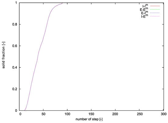
Figure 11. Solid phase growth obtained for selected point in casting domain. Solid phase fraction for multiplication factor $m=15$ calculated by mixed time partitioning methods.

Figure 12. Standard deviation. Average temperature and standard deviation for multiplication factor $m=1$.

Finally, we compare the temperature and solid fraction distributions in the casting between different configurations. In Figure 13, we depict the solid phase fraction distribution after $37.5$ s, that is, more or less in the middle of the casting solidification. In Figure 14 the map of solid phase fraction in casting domain after $37.5$ s is presented. In Figure 15, we depict the temperature distribution in the casting after $67.5$ s, that is, more or less in the middle of the calculations when only part of the casting has already solidified. All the plotted fields agree with our understanding of the modeled phenomena.

Figure 13. Distribution of solid phase fraction in casting domain (red color—liquid state, blue color—solid state). Four combination of the time integration schemes (A) $I-I^m$, (B) $E-E^m$, (C) $E-I^m$, (D) $I-E^m$ for multiplication factor $m=15$.

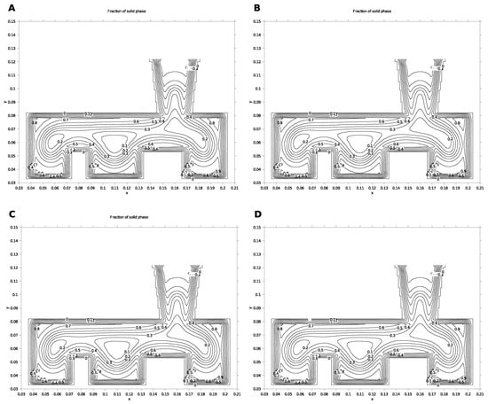
Figure 14. Solid phase fraction in whole casting domain. Four combination of the time integration schemes (A) $I-I^m$, (B) $E-E^m$, (C) $E-I^m$, (D) $I-E^m$ for multiplication factor $m=1$.

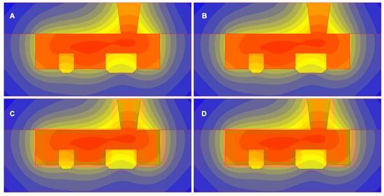
Figure 15. Temperature field in whole domain (a shade of red color—the highest temperature, connected with the cast and a blue color—the lowest temperature). Four combination of the time integration schemes (A) $I-I^m$, (B) $E-E^m$, (C) $E-I^m$, (D) $I-E^m$ for multiplication factor $m=15$.

In the final analysis, we may see that the use of implicit time integration method increases the computational time but allows to use larger time step. However, one should be careful as too large size of time step may lead to the oversight of some important physical phenomena (e.g., solid phase fraction) or lead to significant errors. We purposefully chose the multiplication factor m larger than the acceptable value (determine in accordance with stability criterion described in Section 2.1.2) and indeed got erroneous results—the incorrect distribution of the temperature and solid phase fraction (see Figure 16).

Figure 16. Erroneous results. Errors appearing in computational results for (A) temperature and (B) solid phase fraction are caused by too large the time step (e.g., in the explicit scheme or when multiplication factor $m>15$). There were occurred at the interface between the mold and the cast. Contrasting colors (blue in A, and red in B) denote incorrect values of solid phase fraction.

In conclusion, we showcased that using mixed time partitioning methods indeed offers significant gains. We demonstrate more than three times improvements of computational efficiency compared to the standard approach.

4. Conclusions

In this paper, we have proposed a mixed time partitioning method. We have tested several variants with a different combination of time integration schemes, but also various choices of the size of the time step. In particular, we performed a series of tests and made several important observations:

• We were the first to show that it is possible to use a mixed time partitioning method with various combination of schemes during the numerical simulations of solidification. Moreover, we have shown that different time steps can be chosen for different sub-domains demonstrating that the stability condition for one sub-domain does not enforce the same time step for all domains.
• We have demonstrated that the method presented here offers significant improvements in computational studies of solidification. We have shown that an increasing efficiency depends on the choice of time integration schemes and multiplication m factor,
• We have rigorously shown that the accuracy of the numerical solution is not too affected, as long as stability condition is satisfied.
• Finally, we note that the method presented here does not require specialized hardware or sophisticated algorithms. It can be relatively easy explored on desktop stations commonly available in the foundry and metallurgical manufacture.

References

- Kim, J.; Sandberg, R. Efficient parallel computing with a compact finite difference scheme. Comput. Fluids 2012, 58, 70–87. [Google Scholar] [CrossRef]
- Michalski, G.; Sczygiol, N. Using CUDA Architecture for the Computer Simulation of the Casting Solidification Process. In Proceedings of the International MultiConference of Engineers and Computer Scientists: Lecture Notes in Engineering and Computer Science, Hong Kong, China, 12–14 March 2014; pp. 933–937. [Google Scholar]
- Strzodka, R.; Dogger, M.; Kolb, A. Scientific computation for simulations on programmable graphics hardware. Simul. Model. Pract. Theory 2005, 13, 667–680. [Google Scholar] [CrossRef]
- Wyrzykowski, R.; Szustak, L.; Rojek, K. Parallelization of 2D MPDATA EULAG Algorithm on Hybrid Architectures with GPU accelerators. Parallel Comput. 2014, 40, 425–447. [Google Scholar] [CrossRef]
- Yang, N.; Li, D.; Zhang, J.; Xi, Y. Model predictive controller design and implementation on FPGA with application to motor servo system. Control Eng. Pract. 2012, 20, 1229–1235. [Google Scholar] [CrossRef]
- Heineken, W.; Warnecke, G. Partitioning methods for reaction-diffusion problems. Appl. Numer. Math. 2006, 56, 981–1000. [Google Scholar] [CrossRef]
- Le Bars, M.; Worster, M.G. Solidification of a binary alloy: Finite-element, single-domain simulation and new benchmark solutions. J. Comput. Phys. 2006, 216, 247–263. [Google Scholar] [CrossRef][Green Version]
- Belytschko, T.; Lu, Y.Y. Convergence and stability analyses of multi-time step algorithm for parabolic systems. Comput. Methods Appl. Mech. Eng. 1993, 102, 179–198. [Google Scholar] [CrossRef]
- Cho, Y.G.; Kim, J.Y.; Cho, H.H.; Cha, P.R.; Suh, D.W.; Lee, J.K.; Han, H.N. Analysis of Transformation Plasticity in Steel Using a Finite Element Method Coupled with a Phase Field Model. PLoS ONE 2012, 7, e35987. [Google Scholar] [CrossRef] [PubMed]
- Gravouil, A.; Combescure, A. Multi–time–step explicit–implicit method for non–linear structural dynamics. Int. J. Numer. Methods Eng. 2001, 50, 199–225. [Google Scholar] [CrossRef]
- Smolinski, P.; Palmer, T. Procedures for multi–time step integration of element–free galerkin methods for diffusion problems. Comput. Struct. 2000, 77, 171–183. [Google Scholar] [CrossRef]
- Stefanescu, D.M. Science and Engineering of Casting Solidification; Kluwer Academic: New York, NY, USA, 2002. [Google Scholar]
- Wu, Y.; Smolinski, P. A multi–time step integration algorithm for structural dynamics based on the modified trapezoidal rule. Comput. Methods Appl. Mech. Eng. 2000, 187, 641–660. [Google Scholar] [CrossRef]
- Sczygiol, N. Approaches to enthalpy approximation in numerical simulation of two–component alloy solidification. Comput. Assist. Mech. Eng. Sci. 2000, 7, 717–734. [Google Scholar]
- Sczygiol, N. Numerical Modelling of Thermo-Mechanical Phenomena in Solidifying Cast and Casting Mould, Monographs no. 71 ed.; Czestochowa University of Technology: Czestochowa, Poland, 2000. (In Polish) [Google Scholar]
- Ye, C.; Shi, J.; Cheng, G. An eXtended Finite Element Method (XFEM) study on the effect of reinforcing particles on the crack propagation behavior in a metal–matrix composite. Int. J. Fatigue 2012, 44, 151–156. [Google Scholar] [CrossRef]
- Feulvarch, E.; Roux, J.; Bergheau, J. Finite element solution for diffusion–convection problems with isothermal phase changes. C. R. Mécanique 2012, 340, 512–517. [Google Scholar] [CrossRef]
- Kupczik, K.; Lev-Tov Chattah, N. The Adaptive Significance of Enamel Loss in the Mandibular Incisors of Cercopithecine Primates (Mammalia: Cercopithecidae): A Finite Element Modelling Study. PLoS ONE 2014, 9, e97677. [Google Scholar] [CrossRef] [PubMed]
- Olofsson, J.; Svensson, I. Incorporating predicted local mechanical behaviour of cast components into finite element simulations. Mater. Des. 2012, 34, 494–500. [Google Scholar] [CrossRef]
- Sczygiol, N.; Nagorka, A.; Szwarc, G. NuscaS original software for modelling of thermomechanics phenomena. In Polska Metalurgia w Latach 1998–2002; Swiatkowski, R., Ed.; Wyd. Naukowe AKAPIT: Krakow, Poland, 2002; Volume 2, pp. 243–249. (In Polish) [Google Scholar]
- Zienkiewicz, O.C.; Taylor, R.L. The Finite Element Method; Butterworth-Heinemann: Oxford, UK, 2000; Volume 1. [Google Scholar]
- Wood, L.W. Practical Time-Stepping Schemes; Clarendon Press: Oxford, UK, 1990. [Google Scholar]
- Gawronska, E.; Sczygiol, N. Relationship between eugenvalues and size of time step in computer simulation of thermomechanics phenomena. In Proceedings of the International MultiConference of Engineers and Computer Scientists: Lecture Notes in Engineering and Computer Science, Hong Kong, China, 12–14 March 2014; pp. 881–885. [Google Scholar]
- Gawronska, E.; Sczygiol, N. Application of mixed time partitioning methods to raise the efficiency of solidification modeling. In Proceedings of the 12th International Symposium on Symbolic and Numeric Algorithms for Scientific Computing (SYNASC 2010), Timisoara, Romania, 23–26 September 2010; pp. 99–103. [Google Scholar]
- Gawronska, E.; Sczygiol, N. Numerically Stable Computer Simulation of Solidification: Association between Eigenvalues of Amplification Matrix and Size of Time Step. In Transactions on Engineering Technologies; Springer: Dordrecht, The Netherlands, 2015; pp. 17–30. [Google Scholar]
- Dyja, R.; Mikoda, J. 3D simulation of alloy solidification in the NuscaS system. Sci. Res. Inst. Math. Comput. Sci. 2011, 10, 33–40. [Google Scholar]
- Skrzypczak, T. Sharp interface numerical modeling of solidification process of pure metal. Arch. Metall. Mater. 2012, 57, 1189–1199. [Google Scholar] [CrossRef]
© 2019 by the author. Licensee MDPI, Basel, Switzerland. This article is an open access article distributed under the terms and conditions of the Creative Commons Attribution (CC BY) license (http://creativecommons.org/licenses/by/4.0/).