Field Navigation Using Fuzzy Elevation Maps Built with Local 3D Laser Scans

Abstract

The paper describes the case study of the mobile robot Andabata navigating on natural terrain at low speeds with fuzzy elevation maps (FEMs). To this end, leveled three-dimensional (3D) point clouds of the surroundings are obtained by synchronizing ranges obtained from a 360${}^{\circ }$ field of view 3D laser scanner with odometric and inertial measurements of the vehicle. Then, filtered point clouds are employed to produce FEMs and their corresponding fuzzy reliability masks (FRMs). Finally, each local FEM and its FRM are processed to choose the best motion direction to reach distant goal points through traversable areas. All these tasks have been implemented using ROS (Robot Operating System) nodes distributed among the cores of the onboard processor. Experimental results of Andabata during non-stop navigation on an urban park are presented.

1. Introduction

Autonomous navigation of unmanned ground vehicles (UGVs) requires detailed and updated information on the environment obtained from onboard sensors [1]. Laser rangefinders are sensors commonly employed to obtain three-dimensional (3D) point clouds of the area where the mobile robot moves. Thus, these kinds of sensors are used by UGVs for off-road navigation [2], for planetary exploration [3], urban search and rescue [4] or for agricultural applications [5].

The processing of outdoor scenes acquired with a 3D laser scanner is very different from object scanning [6], since in any direction and at any distance relevant data can be found. In addition, there may be more occlusions, erroneous ranges or numerous points from unconnected areas. In urban areas and indoors, processing of laser information can benefit from the recognition of common geometric features, such as planes [7]. Natural terrain classification can be performed by computing saliency features that capture the local spatial distribution of 3D points [8,9].

In past years, 3D data acquisition from UGVs was usually performed in a stop-and-go manner [10,11], but, nowadays, it can be performed in motion by using some kind of simultaneous localization and mapping (SLAM) by combining data from odometry [12] or from an inertial unit [13].

A leveled 3D point cloud is a representation of the surroundings that can be used for local navigation [14]. Elevation maps offer a compact way of representing 3D point clouds with a $2.5$-dimensional data structure [15]. Moreover, fuzzy elevation maps (FEMs) can operate with measurement uncertainty of the sensors [16,17]. However, fuzzy interpolation can produce unreliable solutions in areas with sparse measurements, and it is necessary to use a fuzzy reliability mask (FRM) for each FEM [18,19].

Navigation on natural terrains can be performed by following distant goal points given by their geographic coordinates [20,21]. These waypoints can be planned based on 2D terrestrial maps or aerial images [22], and represents the trajectory that, broadly, the vehicle should follow. However, to navigate between distant goal points, the robot must avoid local obstacles [23]. For this purpose, reactive navigation based on the evaluation of elementary movements in terms of the risks of traversing the terrain have been proposed [24,25,26].

This paper describes a case study of outdoor navigation using FEMs with the mobile robot Andabata (see Figure 1). All in all, the paper offers three main contributions:

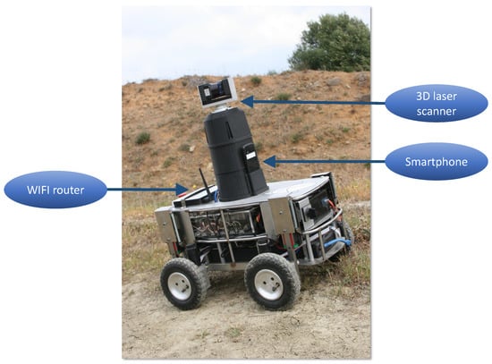
Figure 1. The Andabata mobile robot with the 3D laser scanner on top.

• A complete field navigation system developed on the onboard computer under the Robot Operating System (ROS) [27] is presented.
• 3D scan acquisition with a continuous rotating 2D laser scanner [28] is performed with a local SLAM scheme during vehicle motion.
• The computation of FEMs and FRMs is sped up using least squares fuzzy modeling [29] and multithreaded execution of nodes among the cores of the processor.

The paper is organized as follows. The next section presents the mobile robot Andabata including its 3D laser sensor. Section 3 explains how leveled 3D point clouds are obtained while the robot is moving. Then, Section 4 details the filter applied to the leveled 3D point cloud. The construction of the FEM and FRM with the filtered 3D point cloud is described in Section 5. The multithreaded computing of FEMs and FRMs under ROS is discussed in Section 6. Section 7 presents the field navigation strategy of Andabata and some experimental results. The paper ends with conclusions, acknowledgements and references.

2. The Mobile Robot Andabata

Andabata is an outdoor mobile robot that weighs 41 $\mathrm{k}\mathrm{g}$ and is powered by batteries. The maximum dimensions of the robot are $0.67\mathrm{m}$ long, $0.54\mathrm{m}$ wide and $0.81\mathrm{m}$ high (see Figure 1).

Andabata consists of a skid-steered vehicle with four 20 $\mathrm{cm}$ diameter wheels. Each wheel has a passive suspension system (with two springs and a linear guide with a stroke of $6.5\mathrm{c}\mathrm{m}$) and is actuated by its own direct-current motor with an encoder and a gearbox. The motors are driven by two dual Sabertooth power stages connected to two dual Kangaroo controllers. These controllers receive speed commands for the left and right treads and send motor encoder measurements via an USB port to the computer (see Figure 2). The maximum speed of the vehicle is $v_{max}=0.68\mathrm{m}{\mathrm{s}}^{-1}$ during straight line motion, but decreases to zero as the turning radius reduces.

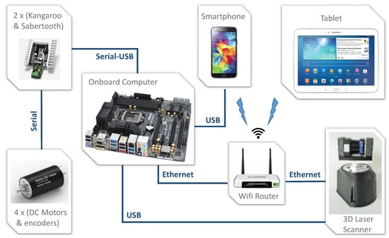
Figure 2. Communication between hardware components of Andabata.

The chassis of the robot has three levels: bottom for the motors and the battery, middle for electronics and the computer, and top for sensors and a WiFi router (see Figure 1). The computer has an Intel Core processor i7 4771 (four cores, $3.5\mathrm{GHz}$, 8 MB cache) and 16 GB RAM. A tablet is used for remote supervision and teleoperation of the robot via the onboard WiFi router (see Figure 2). Andabata has a smartphone to obtain data from its GPS (with a horizontal resolution of 10 $\mathrm{m}$), inclinometers, gyroscopes, magnetometers and its camera.

In addition, the robot has a 3D laser rangefinder (see Figure 1), built from a two-dimensional (2D) scanner Hokuyo UTM-30LX-EW [28]. Power and data transmission between the base and the head is carried out by a slip ring that allows unconstrained rotation. The range of measurements varies from $0.1\mathrm{m}$ to 30 $\mathrm{m}$ (reduced to 15 $\mathrm{m}$ with direct sunlight). The 3D sensor has the same vertical resolution of the 2D scanner (i.e., ${0.25}^{\circ }$). The horizontal resolution can be selected by modifying the rotation speed of the head. The blind zone of the 2D sensor is 90^∘, which is located below to avoid interferences with the robot. Thus, the blind zone for the 3D laser rangefinder is a cone with the radius of the base equal to the height h = $0.723\mathrm{m}$ of its optic centre above the floor.

Andabata can be teleoperated by a person through an Android app in the tablet called Andabata, which is an adaptation of the Mover-bot app [30] that runs both on the tablet and the onboard smartphone. The application on the tablet has two sliders for both hands to indicate the speed of the left and right treads, which are sent through the local WiFi network to the Andabata app on the smartphone (see Figure 3). Video feedback, GPS position, and robot inclination is provided by the smartphone to the tablet via WiFi. Another app on the smartphone, called Android_sensors_driver, publishes a ROS topic directly on the computer with all the sensory data of the smartphone via WiFi [31].

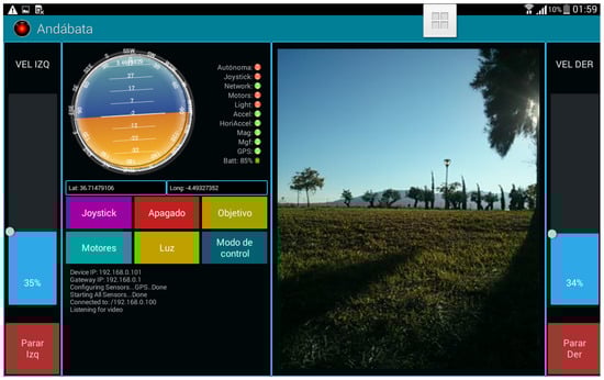
Figure 3. User interface of the Android app $Andabata$ on the tablet.

Figure 4 shows a general scheme of the ROS nodes employed by Andabata. The Navigation_mode node selects tread commands from teleoperation or from autonomous navigation, which are sent to the motor drivers through the Motor_control node. During teleoperation, the Andabata app on the smartphone retransmits the speed commands from the tablet to the Teleoperation node via USB. The rest of ROS nodes are explained in the following sections.

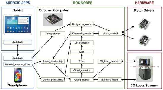
Figure 4. Software scheme of Andabata.

3. Obtaining Leveled 3D Point Clouds

This section describes the acquisition of leveled 3D point clouds on Andabata while moving on irregular terrain. For this purpose, it is necessary to synchronize the motion of the vehicle with 2D scan acquisition. All in all, it represents a local SLAM scheme implemented at low speeds without loop closures.

Let $XYZ$ be the reference system associated with the robot, which is located at the geometric center of the rectangle defined by the contact points of the wheels with the ground. The X-axis coincides with the longitudinal axis of the vehicle pointing forwards, the Z-axis is normal to the support plane and points upwards and the Y-axis completes this orthogonal coordinate system pointing to the left (see Figure 5). The Cartesian coordinates for a leveled 3D point cloud are expressed in an $X_p{Y}_p{Z}_p$ reference system whose origin coincides with that of the vehicle at the beginning of each scan. The $X_p$ axis coincides with the projection of X on the horizontal plane, $Y_p=Y$ and $Z_p$ is defined with the same direction as gravity and opposite direction (see Figure 5).

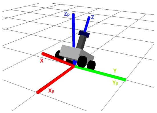
Figure 5. Reference systems for the robot ($XYZ$) and for a leveled 3D scan ($X_p{Y}_p{Z}_p$).

The Kinematic_model node is in charge of calculating the actual longitudinal and angular velocities of the vehicle (see Figure 4). For this purpose, it employs the encoder readings of the motors (obtained by the Motor_control node from the motor drivers) on an approximate 2D kinematic model of skid-steering [32].

The Local_positioning node employs an unscented Kalman filter [33] to localize the vehicle with respect to $X_p{Y}_p{Z}_p$ during the acquisition of the whole 3D scan. To this end, the node merges the roll and pitch angles, the yaw speed of the vehicle (provided by the smartphone and published by the Android_sensors_driver app), and the linear and angular velocities from the Kinematic_model node.

For 3D laser scan acquisition, the Spinning_head node commands a constant rotation speed for the head and periodically receives (every 25 ms) the relative angle between the head and the base at the start of each 2D scan via the USB connection. In this way, this node can publish the transformation between the 2D laser sensor reference system and $XYZ$. In addition, the 2D_laser_scanner node allows for configuring the Hokuyo sensor and publishes the 2D scans that the computer receives through the Ethernet connection.

Finally, the Cloud_maker node publishes the 3D leveled point cloud by combining the successive 2D vertical scans (published by the 2D_laser_scanner node) with the relative transformations between the reference system of the 2D laser scanner and $XYZ$ (provided by the Spinning_head node), and between $XYZ$ and $X_p{Y}_p{Z}_p$ (published by the Local_positioning node).

With Andabata stopped, a 180${}^{\circ }$ horizontal turn of the head of the 3D scanner is enough to capture all the surroundings of the robot, but, with the vehicle in motion, it is necessary to perform a full 360${}^{\circ }$ turn. In this way, non-sampled areas around the robot are avoided and the blind zone above the robot is reduced (see Figure 6).

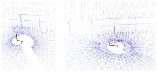
Figure 6. Details of leveled 3D laser scans obtained with a sensor’s head rotation of 180^∘ (left) and 360^∘ (right) while Andabata was moving along a slope.

4. Filtering 3D Point Clouds

To build useful FEMs and FRMs, it is necessary to filter the leveled 3D point clouds. Filtering is composed of three consecutive steps: far points elimination, overhangs removal and maximum height normalization. These steps are performed by the Filter node, and its output is processed by the Map node (see Figure 4).

The first step is to eliminate far points, concretely those whose projection on the horizontal plane is far from $d_{max}$= 10 $\mathrm{m}$ from the origin of the 3D scan. The reason for this is the low visibility of the ground from the point of view of the 3D laser scanner, which is limited to h on Andabata (see Section 2) and because distant zones are sampled with a lower density than closer ones. In addition, the number of points to be processed is reduced and the resulting 3D point cloud focuses on the area where the next movements of the vehicle will take place.

Overhangs that do not constitute an obstacle for Andabata, such as the ceiling of a tunnel or tree canopy, need to be removed. For this purpose, the second step of the filter employs the collapsible cubes method with coarse binary cubes with an edge of E = $0.5\mathrm{m}$ [34]. Basically, occupied 3D cubes above a minimum vertical gap are omitted. Thus, points inside unsupported cubes are eliminated from the point cloud. Two empty cubes are enough for Andabata to navigate safely below overhangs.

In the third step, the maximum height of obstacles is limited to 3 $\mathrm{m}$ above the ground. The objective for this step is that the height of tall and small obstacles can be comparable. For this purpose, the z-coordinates of 3D points inside coarse cubes with five or more cubes above its vertical ground cube are lowered.

Figure 7 shows a leveled 3D scan obtained while Andabata was moving in an urban park (see Figure 8). It can be observed in Figure 7 that far points (blue) and overhangs from the canopy of the trees (green) are discarded from the filtered 3D scan (red). It is also noticeable that the maximum height of the trees has been limited.

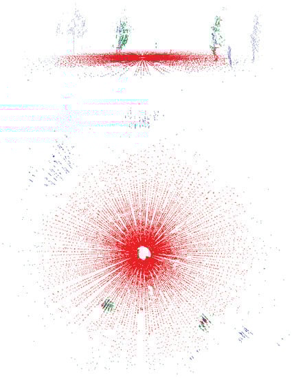
Figure 7. Lateral (top) and aerial views (bottom) of a filtered 3D point cloud (red) obtained from a leveled 3D point cloud. Blue and green colors represent far points and overhangs, respectively.

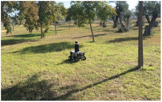
Figure 8. Andabata navigating on an urban park.

5. Building FEMs and FRMs

This section describes the computation of an FEM and its FRM from a filtered 3D point cloud. Instead of using the adaptive neuro-fuzzy inference system (ANFIS) for identification [16,18,19], least squares fuzzy modeling [29] has been employed to improve computation time. Additionally, cylindrical coordinates $(\alpha ,r,z)$ have been employed instead of Cartesian coordinates $(x,y,z)$.

It is assumed that the ground surface around the robot can be represented as a continuous function $z=H(\alpha ,r)$, where the angle $\alpha =arctan(y/x)$ and the distance $r=\sqrt{x^2+y^2}$ describe the projection of a 3D point on the $X_p{Y}_p$ plane. Similarly, an FRM is defined as a continuous function $v=V(\alpha ,r)$, where values of v close to one and zero, represent the maximum and minimum reliability values for the FEM, respectively. The FEM and FRM are defined in the universe $U_{\alpha }=[0{}^{\circ },360{}^{\circ }]$ for variable $\alpha$, and $U_r=[0\mathrm{m},d_{max}]$ for r, which corresponds to a circle centered at the origin of $X_p{Y}_p$.

A total of sixteen fuzzy sets for $\alpha$ have been defined evenly-distributed over $U_{\alpha }$ (see Figure 9). In this case, triangular membership functions ${\mu }_i$ for $i=1,2,\cdots ,16$ are defined as:

$${\mu }_i\left(\alpha \right)=\left\{\begin{array}{cc}\frac{\alpha -{\alpha }^{i-1}}{{\alpha }^i-{\alpha }^{i-1}},\hfill & \mathrm{if}{\alpha }^{i-1}\le \alpha <{\alpha }^i,\hfill \\ \frac{{\alpha }^{i+1}-\alpha }{{\alpha }^{i+1}-{\alpha }^i},\hfill & \mathrm{if}{\alpha }^i\le \alpha <{\alpha }^{i+1},\hfill \\ 0,\hfill & \mathrm{otherwise},\hfill \end{array}\right.$$

(1)

where ${\alpha }^i=(i-1)22.5{}^{\circ }$ represent the peak values, i.e., ${\mu }_i\left({\alpha }^i\right)=1$.

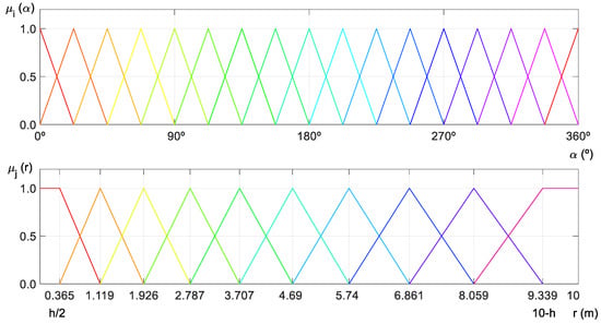
Figure 9. Membership functions for variables $\alpha$ (top) and r (bottom).

For distance r, ten uneven-distributed fuzzy sets have been defined over $U_r$ to provide higher detail for regions closest to the robot (see Figure 9). Concretely, peak parameter $r^j$ for $j=1,2,\cdots 10$ are computed as:

$$r^j=\left(\frac{{\tau }^j-1}{{\tau }^{10}-1}\right)\left(d_{max}-\frac{h}{2}\right)-\frac{h}{2},$$

(2)

where $\tau =1.0624$ is an expansion ratio that fulfills that $r^1=h/2$. Then, the membership functions ${\mu }_j$ for r are defined as:

$${\mu }_j\left(r\right)=\left\{\begin{array}{cc}1,\hfill & \mathrm{if}r\le r^1\mathrm{or}r\ge r^{10},\hfill \\ \frac{r-r^{j-1}}{r^j-r^{j-1}},\hfill & \mathrm{if}{r}^{j-1}\le r<r^j,\hfill \\ \frac{r^{j+1}-r}{r^{j+1}-r^j},\hfill & \mathrm{if}{r}^j\le r<r^{j+1},\hfill \\ 0,\hfill & \mathrm{otherwise}.\hfill \end{array}\right.$$

(3)

The combined membership for both variables ${\mu }_{i,j}$ is calculated with the product operator for a given 3D point:

$${\mu }_{i,j}(\alpha ,r)={\mu }_i\left(\alpha \right){\mu }_j\left(r\right),$$

(4)

where the following condition is satisfied:

$$\sum _{\forall i,j}{\mu }_{i,j}(\alpha ,r)=1.$$

(5)

Let m be a row vector that contains all the possible memberships:

$$m(\alpha ,r)=\left({\mu }_{1,1}(\alpha ,r),{\mu }_{1,2}(\alpha ,r),\cdots ,{\mu }_{16,10}(\alpha ,r)\right),$$

(6)

where most of its 160 elements are null. Non null elements correspond to the regions where the projection of the 3D point falls on the $X_p{Y}_p$ plane and its nearby regions (see Figure 10).

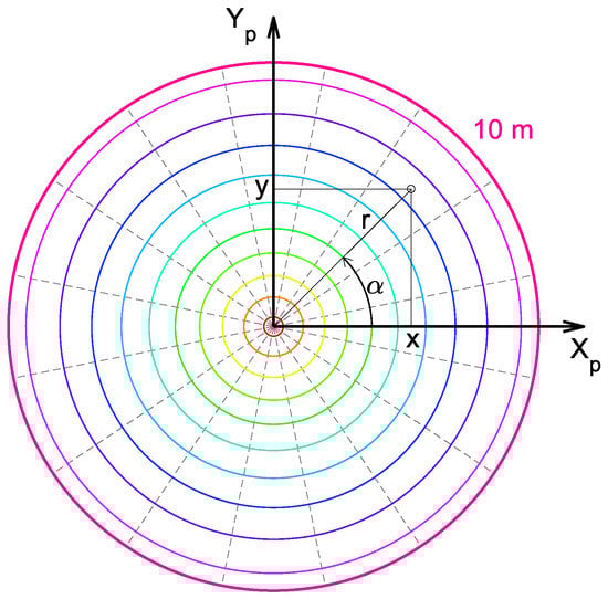
Figure 10. Regions defined by the fuzzy membership functions.

Using zero-order Sugeno consequents for the rule that relates the fuzzy set i for $\alpha$ and the fuzzy set j for r requires just one parameter $z_{i,j}$ for the FEM, and another $v_{i,j}$ for the FRM. Let ${\theta }_z$ and ${\theta }_v$ be the column vectors that contains all the unknown parameters:

$${\theta }_z=\left(\begin{array}{c}{z}_{1,1}\\ z_{1,2}\\ ⋮\\ z_{16,10}\end{array}\right),{\theta }_v=\left(\begin{array}{c}{v}_{1,1}\\ v_{1,2}\\ ⋮\\ v_{16,10}\end{array}\right).$$

(7)

Given the algebraic equations: $z=m(\alpha ,r){\theta }_z$ and $1=m(\alpha ,r){\theta }_v$ for the FEM and the FRM, respectively, the least-squares method finds the parameters ${\theta }_z$ and ${\theta }_v$, respectively, that minimizes the sum of the squares of the residuals: $z-m(\alpha ,r){\theta }_z$ and $1-m(\alpha ,r){\theta }_v$, respectively, made in the results of every 3D point in cylindrical coordinates $(\alpha ,r,z)$.

For model training, the recursive least squares technique has been employed in the Map node. At first, ${\theta }_z$ and ${\theta }_v$ are initialized with zeroes, with the exception of the parameters associated with the first fuzzy set for r, i.e., those numbered $j=1$. These zones may not contain any 3D point due to the blind zone of the 3D laser scanner. Thus, the parameters $z_{i,1}$ are filled with the heights deduced from the pitch and roll angles of the mobile robot at $X_p{Y}_p{Z}_p$. Additionally, for all i, $v_{i,1}=1$ to indicate that these zones on the FEM are reliable because Andabata has already been on them.

To obtain ${\theta }_z$, recursive least squares equations are:

$$L_1=\frac{P_1{m}^T}{1+m^T{P}_{1}m},{\theta }_z={\theta }_z+L_1(z-m{\theta }_z),P_1=P_1-L_{1}m{P}_1,$$

(8)

where $L_1$ is a gain vector and $P_1$ is the covariance matrix, which is chosen initially as the identity matrix multiplied by a big positive number to indicate that there is no confidence on the initial $z_{i,j}$ parameters. Similarly, to calculate ${\theta }_v$ , the recursive equations are:

$$L_2=\frac{P_2{m}^T}{1+m^T{P}_{2}m},{\theta }_v={\theta }_v+L_2(1-m{\theta }_v),P_2=P_2-L_{2}m{P}_2,$$

(9)

where $L_2$ and $P_2$ are the gain vector and the covariance matrix, respectively. Initially, $P_2$ is chosen as the identity matrix multiplied by a small positive number to indicate that there is confidence on the initial $v_{i,j}$ parameters (which means no reliability on the initial FEM).

Once identified the fuzzy parameters in ${\theta }_z$ and ${\theta }_v$, it is possible to estimate for every $(\alpha ,r)$ the height on the FEM: $\widehat{z}=m(\alpha ,r){\theta }_z$ and the reliability value on the FRM: $\widehat{v}=m(\alpha ,r){\theta }_v$. Figure 11 shows the FEM and the FRM obtained from the filtered 3D point cloud represented in Figure 7.

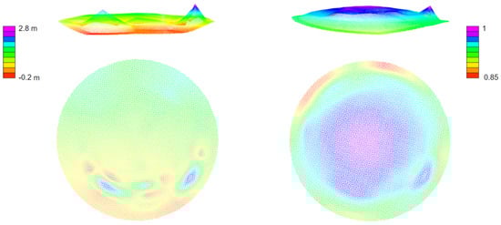
Figure 11. Lateral (top) and aerial views (bottom) of the FEM (left) and FRM (right) associated with the filtered 3D point cloud of Figure 7.

6. Multithreaded Computation of FEMs and FRMs

The onboard computer of Andabata has a processor with four physical cores, but it employs simultaneous multithreading to divide each core into two virtual units, resulting in eight independent virtual cores. This section discusses how to employ the multithreading capability of ROS in the virtual cores to enhance the output rate and steadiness of FEMs and FRMs.

With an horizontal resolution of ${2.4}^{\circ }$ for the 3D laser scanner, a filtered 3D point cloud is obtained every $3.75\mathrm{s}$, with $60,000$ laser points approximately (this number depends heavily on sky visibility, that reduces the number of valid ranges). However, the calculation of the FEM and its FRM (performed by the Map node) takes much more time. This time depends on the total number of 3D points and on the processor load.

To increase the output rate, the calculation of the FEM and the FRM has been parallelized into two threads inside the Map node by separating the calculation of Equation (8) to that of Equation (9). For further improvement, the Map node can be launched two or more times working on different 3D point clouds.

To decide which 3D point clouds will be processed and which will be discarded, the Cloud_selector node has been developed (see Figure 4). When a Map node becomes available, it is necessary to decide to employ the previous received 3D point cloud or to wait for the reception of the current 3D point cloud. Moreover, in case of using multiple Map nodes, it can also be of interest to wait for future 3D scans to avoid the processing of consecutive 3D laser scans (introducing one or more spacing).

Figure 12 and Figure 13 show timetables with the output rates of the 3D point clouds, FEMs and FRMs using the previous and actual 3D scans, respectively. In these figures, different selection strategies have been employed by the Cloud_selector node. Processed 3D point clouds are colored and the same color is employed to indicate when its corresponding FEM and FRM have been obtained. Discarded 3D point clouds are not colored at all.

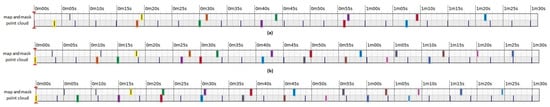
Figure 12. Output rate for the 3D point cloud, FEM and FRM using the last received 3D point cloud with one Map node (a), two Map nodes without forced spacing (b) and two Map nodes with one forced spacing (c).

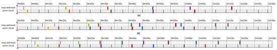
Figure 13. Output rate for the 3D point cloud, FEM and FRM using the current 3D point cloud with one Map node (a), two Map nodes without forced spacing (b) and two Map nodes with one forced spacing (c).

Table 1 compares the map age (i.e., the time employed to produce an FEM and its FRM from a filtered 3D point cloud), the interval between consecutive maps and their respective standard deviations for different selection strategies. When using the current 3D point cloud, the age of the map is smaller, but the interval between maps is greater than when using the previous 3D point cloud. The best map age can be obtained by processing the current 3D point cloud with only one Map node. On the other hand, map interval can be improved by using more Map nodes. The ideal strategy would be the one that minimizes both map age and map interval. A compromise between both objectives can be achieved by using two Map nodes and one forced spacing with the previous point cloud. Consequently, the latter is the selection strategy adopted for autonomous navigation of Andabata.

Table 1. Comparison between different multithreaded strategies.

3D Point	Map	Forced	Map	Standard	Map	Standard
Cloud	Nodes	Spacing	Age (s)	Deviation (s)	Interval (s)	Deviation (s)
previous	1	0	14.20	1.31	12.56	0.48
	2	0	18.21	1.90	8.27	5.76
		1	15.30	1.08	7.45	1.37
		2	15.73	1.62	11.37	0.50
	3	0	27.34	3.41	6.60	6.09
		1	20.21	0.45	7.55	0.77
		2	23.95	2.11	11.13	2.30
current	1	0	13.81	0.68	14.91	0.98
	2	0	14.83	1.79	8.36	4.50
		1	15.21	1.33	8.13	2.20
		2	12.06	1.58	11.70	2.40
	3	0	28.44	4.16	6.88	2.65
		1	20.89	1.24	7.70	0.98
		2	23.18	0.72	11.35	0.59

7. Field Navigation

A navigation mission for Andabata is defined by an ordered list of distant goal points, each one determined by its latitude and longitude coordinates. The navigation strategy consists of approaching the goal points while avoiding local obstacles reactively. The mission will end either when the last goal point is reached (mission completion) or when the roll or pitch angles of the vehicle surpass 20^∘ (mission failure due to excessive inclination).

The ROS package actionlib [35] has been used to implement this navigation strategy, since the mission takes a long time to be completed and it should be able to be canceled or interrupted at any time.

7.1. Global Localization

The relative position and orientation of the mobile robot with respect to the current goal point are obtained by the Global_positioning node. This node process the data of the GPS and magnetometers of the smartphone published by the Android_sensors_driver app (see Figure 4).

Before starting navigation, it is necessary to calibrate the magnetometers of the smartphone, since their measurements can be affected by the environment and by the mobile robot itself. Calibration consists of turning the robot on spot during one full turn on horizontal plane with lateral motor speed of the same magnitude but different sign. Then, the magnetic measurements on the X and Y axes, $B_x$ and $B_y$, respectively, are adjusted to resemble a circumference (see Figure 14).

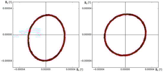
Figure 14. Magnetic field measurements before (left) and after calibration (right).

Afterwards, the orientation of the vehicle with respect to the north, i.e., the yaw, can be obtained during navigation as:

$$yaw=arctan\left(\frac{B_x}{B_y}\right),$$

(10)

and the relative orientation of the vehicle with respect to the current goal point can be deduced.

When the distance between the current position of Andabata (given by its GPS coordinates) and the goal point is smaller than 10 $\mathrm{m}$ (that corresponds to the GPS horizontal resolution), the goal point is considered already visited and the next goal point from the mission list becomes the current goal point.

7.2. Direction Selection

Every time an FEM and its FRM are delivered by a Map node, the Dir_selection node computes a new motion direction (see Figure 4). A total of 32 possible directions $d_i$ from the projection of the current $XYZ$ frame onto the $X_p{Y}_p$ plane are checked (see Figure 15). The chosen direction $d_j$ will be the one that minimizes the following cost function:

$$J\left(d_i\right)=\frac{|{\Delta }_i|+g|{\delta }_i|}{D_i},$$

(11)

where ${\Delta }_i$ is the difference between $d_i$ and the goal point direction, ${\delta }_i$ is the angular difference between $d_i$ and the projection of the X-axis, $g=0.02$ is a factor that penalizes changes of direction, and $D_i$ is the maximum distance that the robot could travel over the FEM following $d_i$ (see Figure 15).

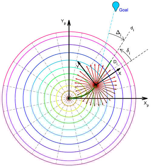
Figure 15. Illustration of direction selection over the FEM.

To compute $D_i$, several points $(x,y)$ are evaluated in the FEM and FRM along $d_i$ with steps of $0.1\mathrm{m}$ starting from the current position of the robot. Whenever the checked point has a reliability value on the FRM less than $0.75$, or has a gradient magnitude on the FEM greater than $0.35$, or reach the borders of the FEM, the distance $D_i$, which is initially zero, is not increased more.

The gradient of the FEM $\nabla H$ is employed to detect non traversable areas [18]. The magnitude of the gradient at a point with cylindrical coordinates $(\alpha ,r)$ on the FEM can be calculated as:

$$|\nabla H(\alpha ,r)|=\sqrt{{\left(\frac{\partial H(\alpha ,r)}{\partial x}\right)}^2+{\left(\frac{\partial H(\alpha ,r)}{\partial y}\right)}^2},$$

(12)

where:

$$\begin{array}{c}\hfill \frac{\partial H(\alpha ,r)}{\partial x}=\sum _{\forall i,j}\left[z_{i,j}\left({\mu }_i\left(\alpha \right)\frac{\partial {\mu }_j\left(r\right)}{\partial x}+{\mu }_j\left(r\right)\frac{\partial {\mu }_i\left(\alpha \right)}{\partial x}\right)\right],\end{array}$$

(13)

$$\begin{array}{c}\hfill \frac{\partial H(\alpha ,r)}{\partial y}=\sum _{\forall i,j}\left[z_{i,j}\left({\mu }_i\left(\alpha \right)\frac{\partial {\mu }_j\left(r\right)}{\partial y}+{\mu }_j\left(r\right)\frac{\partial {\mu }_i\left(\alpha \right)}{\partial y}\right)\right],\end{array}$$

(14)

and:

$$\begin{array}{c}\frac{\partial {\mu }_i\left(\alpha \right)}{\partial x}=\left\{\begin{array}{cc}\frac{y}{r^2}\frac{1}{{\alpha }^{i-1}-{\alpha }^i},\hfill & \mathrm{if}{\alpha }^{i-1}\le \alpha <{\alpha }^i,\hfill \\ \frac{y}{r^2}\frac{1}{{\alpha }^{i+1}-{\alpha }^i},\hfill & \mathrm{if}{\alpha }^i\le \alpha <{\alpha }^{i+1},\hfill \\ 0,\hfill & \mathrm{otherwise},\hfill \end{array}\right.\frac{\partial {\mu }_j\left(r\right)}{\partial x}=\left\{\begin{array}{cc}\frac{x}{r}\frac{1}{r^j-r^{j-1}},\hfill & \mathrm{if}{r}^{j-1}\le r<r^j,\hfill \\ \frac{x}{r}\frac{1}{r^j-r^{j+1}},\hfill & \mathrm{if}{r}^j\le r<r^{j+1},\hfill \\ 0,\hfill & \mathrm{otherwise},\hfill \end{array}\right.\hfill \end{array}$$

(15)

$$\begin{array}{c}\frac{\partial {\mu }_i\left(\alpha \right)}{\partial y}=\left\{\begin{array}{cc}\frac{x}{r^2}\frac{1}{{\alpha }^i-{\alpha }^{i-1}},\hfill & \mathrm{if}{\alpha }^{i-1}\le \alpha <{\alpha }^i,\hfill \\ \frac{x}{r^2}\frac{1}{{\alpha }^i-{\alpha }^{i+1}},\hfill & \mathrm{if}{\alpha }^i\le \alpha <{\alpha }^{i+1},\hfill \\ 0,\hfill & \mathrm{otherwise},\hfill \end{array}\right.\frac{\partial {\mu }_j\left(r\right)}{\partial y}=\left\{\begin{array}{cc}\frac{y}{r}\frac{1}{r^j-r^{j-1}},\hfill & \mathrm{if}{r}^{j-1}\le r<r^j,\hfill \\ \frac{y}{r}\frac{1}{r^j-r^{j+1}},\hfill & \mathrm{if}{r}^j\le r<r^{j+1},\hfill \\ 0,\hfill & \mathrm{otherwise}.\hfill \end{array}\right.\hfill \end{array}$$

(16)

7.3. Computing Tread Speeds

Once the motion direction $d_j$ is determined, the commanded angular velocity $\omega$ for Andabata is computed as: $\omega =G{\delta }_j$, where $G=1$ is a proportional gain that regulates heading changes of the vehicle [21]. The longitudinal velocity during navigation v is a constant value that depends on the difficulty of the terrain.

The Dir_selection node sends the desired longitudinal v and angular $\omega$ velocities to the Kinematic_model node, which are converted into left and right tread speeds by using a symmetric inverse kinematic model:

$$v_l=v-y_{ICR}\omega ,v_r=v+y_{ICR}\omega ,$$

(17)

where $y_{ICR}=0.45\mathrm{m}$ is the mean value of tread instantaneous centers of rotation (ICRs) of Andabata on horizontal plane [32]. When any of the tread speeds exceeds their maximum speed $v_{max}$, the commanded speeds (Equation (17)) are divided by:

$$e=\frac{\left|v\right|+y_{ICR}\left|\omega \right|}{v_{max}}.$$

(18)

In this way, the commanded curvature $\gamma$ of the vehicle (and its turning radius) is kept unaltered:

$$\gamma =\frac{\omega /e}{v/e}=\frac{w}{v}.$$

(19)

7.4. Experimental Results

The performance of the navigation system of Andabata has been tested in an urban park with several lampposts, stone benchs and trees (see Figure 8). The park contains soft slopes and different terrains such as grass and sand.

The experiment shown in Figure 16 consists of an outdoor trip from a start point (white cross) to reach two GPS goals (blue dots), which are fulfilled when the robot is closer than 10 $\mathrm{m}$ (red circles). The path followed by Andabata is shown with black dots representing the GPS positions obtained from the onboard smartphone. The longitudinal speed of the robot was set to $v=0.34\mathrm{m}{\mathrm{s}}^{-1}$ and the trip took 540 $\mathrm{s}$, approximately. Figure 16 has been generated with the help of Google Earth [36].

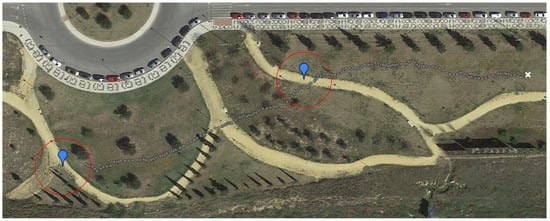
Figure 16. GPS positions of Andabata during navigation (top view).

Changes in the yaw angle during this experiment (obtained with the magnetic compass) can be observed in Figure 17. Remarkable changes occur when the robot tries to aim to the first and second goal points at the beginning and the middle of the trajectory, respectively. Once the goal direction is obtained, some corrections are made in order to cross through traversable areas.

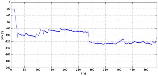
Figure 17. Yaw variations during the experiment.

Figure 18 shows a local FEM and its FRM generated during autonomous navigation. Small black arrows have been superimposed to represent the successive positions of the mobile robot in local coordinates (provided by the Local_positioning node). It can observed how obstacle avoidance is performed while moving towards the goal point.

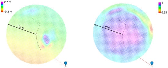
Figure 18. A top view of the local path followed by Andabata (black arrows) over an FEM (left) and its FRM (right).

8. Conclusions

This paper has described the field navigation system of the mobile robot Andabata at low speeds with fuzzy elevation maps (FEMs). For this purpose, the robot obtains leveled three-dimensional (3D) laser scans in motion by integrating ranges from a 360^∘ field of view 3D laser scanner with odometry, inclinometers and gyroscopes. Each leveled 3D scan is employed to produce an FEM and a fuzzy reliability mask (FRM) of the surroundings, which are processed to choose the best motion direction to reach a distant goal point while crossing through traversable areas. This has been implemented with different ROS (Robot Operating System) nodes distributed among the cores of the onboard processor.

It is the first time that a mobile robot navigates with FEMs obtained from 3D laser scans in outdoors. To do so, a complex navigation scheme has been developed by integrating numerous tasks, where it has been necessary to employ 3D point cloud filtering and multithreaded execution to increase the building frequency of FEMs and FRMs. Experimental results of Andabata navigating autonomously in an urban park have been presented.

Work in progress includes navigation in more complicated natural environments and quantitative comparison with state-of-the-art outdoor navigation methods.

References

- Sanfilippo, F.; Azpiazu, J.; Marafioti, G.; Transeth, A.A.; Stavdahl, Ø.; Liljebäck, P. Perception-driven obstacle-aided locomotion for snake robots: the state of the art, challenges and possibilities. Appl. Sci. 2017, 7, 336. [Google Scholar] [CrossRef]
- Larson, J.; Trivedi, M.; Bruch, M. Off-road terrain traversability analysis and hazard avoidance for UGVs. In Proceedings of the IEEE Intelligent Vehicles Symposium (IV), Baden-Baden, Germany, 6 February 2011; pp. 1–7. [Google Scholar]
- Tong, C.H.; Barfoot, T.D.; Dupuis, E. Three-dimensional SLAM for mapping planetary work site environments. J. Field Robot. 2012, 29, 381–412. [Google Scholar] [CrossRef]
- Sinha, A.; Papadakis, P. Mind the gap: Detection and traversability analysis of terrain gaps using LIDAR for safe robot navigation. Robotica 2013, 31, 1085–1101. [Google Scholar] [CrossRef]
- Weiss, U.; Biber, P. Plant detection and mapping for agricultural robots using a 3D LIDAR sensor. Robot. Auton. Syst. 2011, 59, 265–273. [Google Scholar] [CrossRef]
- Chen, L.C.; Hoang, D.C.; Lin, H.I.; Nguyen, T.H. Innovative methodology for multi-view point cloud registration in robotic 3D object scanning and reconstruction. Appl. Sci. 2016, 6, 132. [Google Scholar] [CrossRef]
- Macher, H.; Landes, T.; Grussenmeyer, P. From Point Clouds to Building Information Models: 3D Semi-Automatic Reconstruction of Indoors of Existing Buildings. Appl. Sci. 2017, 7, 1030. [Google Scholar] [CrossRef]
- Lalonde, J.F.; Vandapel, N.; Huber, D.F.; Hebert, M. Natural terrain classification using three-dimensional ladar data for ground robot mobility. J. Field Robot. 2006, 23, 839–861. [Google Scholar] [CrossRef]
- Plaza-Leiva, V.; Gomez-Ruiz, J.A.; Mandow, A.; García-Cerezo, A. Voxel-Based Neighborhood for Spatial Shape Pattern Classification of Lidar Point Clouds with Supervised Learning. Sensors 2017, 17, 594. [Google Scholar] [CrossRef] [PubMed]
- Rekleitis, I.; Bedwani, J.L.; Dupuis, E.; Lamarche, T.; Allard, P. Autonomous over-the-horizon navigation using LIDAR data. Auton. Robots 2013, 34, 1–18. [Google Scholar] [CrossRef]
- Schadler, M.; Stückler, J.; Behnke, S. Rough terrain 3D mapping and navigation using a continuously rotating 2D laser scanner. Künstliche Intell. 2014, 28, 93–99. [Google Scholar] [CrossRef]
- Almqvist, H.; Magnusson, M.; Lilienthal, A. Improving point cloud accuracy obtained from a moving platform for consistent pile attack pose estimation. J. Intell. Robot. Syst. Theory Appl. 2014, 75, 101–128. [Google Scholar] [CrossRef]
- Zlot, R.; Bosse, M. Efficient large-scale three-dimensional mobile mapping for underground mines. J. Field Robot. 2014, 31, 731–752. [Google Scholar] [CrossRef]
- Brenneke, C.; Wulf, O.; Wagner, B. Using 3D Laser range data for SLAM in outdoor environments. In Proceedings of the IEEE International Conference on Intelligent Robots and Systems (IROS), Las Vegas, NV, USA, 27–31 October 2003; Volume 1, pp. 188–193. [Google Scholar]
- Pfaff, P.; Triebel, R.; Burgard, W. An efficient extension to elevation maps for outdoor terrain mapping and loop closing. Int. J. Robot. Res. 2007, 26, 217–230. [Google Scholar] [CrossRef]
- Mandow, A.; Cantador, T.J.; García-Cerezo, A.; Reina, A.J.; Martínez, J.L.; Morales, J. Fuzzy modeling of natural terrain elevation from a 3D scanner point cloud. In Proceedings of the 7th IEEE International Symposium on Intelligent Signal Processing (WISP), Floriana, Malta, 19–21 September 2011; pp. 171–175. [Google Scholar]
- Hou, J.F.; Chang, Y.Z.; Hsu, M.H.; Lee, S.T.; Wu, C.T. Construction of fuzzy map for autonomous mobile robots based on fuzzy confidence model. Math. Probl. Eng. 2014, 2014, 1–8. [Google Scholar] [CrossRef]
- Martínez, J.L.; Mandow, A.; Reina, A.J.; Cantador, T.J.; Morales, J.; García-Cerezo, A. Navigability analysis of natural terrains with fuzzy elevation maps from ground-based 3D range scans. In Proceedings of the IEEE/RSJ International Conference on Intelligent Robots and Systems (IROS), Tokyo, Japan, 3–7 November 2013; pp. 1576–1581. [Google Scholar]
- Mandow, A.; Cantador, T.J.; Reina, A.J.; Martínez, J.L.; Morales, J.; García-Cerezo, A. Building Fuzzy Elevation Maps from a Ground-Based 3D Laser Scan for Outdoor Mobile Robots. In Advances in Intelligent Systems and Computing; Springer: Basel, Switzerland, 2016; Volume 417, pp. 29–41. [Google Scholar]
- Leedy, B.M.; Putney, J.S.; Bauman, C.; Cacciola, S.; Webster, J.M.; Reinholtz, C.F. Virginia Tech’s twin contenders: A comparative study of reactive and deliberative navigation. J. Field Robot. 2006, 23, 709–727. [Google Scholar] [CrossRef]
- Morales, J.; Martínez, J.; Mandow, A.; García-Cerezo, A.; Pedraza, S. Power Consumption Modeling of Skid-Steer Tracked Mobile Robots on Rigid Terrain. IEEE Trans. Robot. 2009, 25, 1098–1108. [Google Scholar] [CrossRef]
- Silver, D.; Sofman, B.; Vandapel, N.; Bagnell, J.A.; Stentz, A. Experimental analysis of overhead data processing to support long range navigation. In Proceedings of the IEEE/RSJ International Conference on Intelligent Robots and System (IROS), Beijing, China, 9–13 October 2006; pp. 2443–2450. [Google Scholar]
- Howard, A.; Seraji, H.; Werger, B. Global and regional path planners for integrated planning and navigation. J. Field Robot. 2005, 22, 767–778. [Google Scholar] [CrossRef]
- Lacroix, S.; Mallet, A.; Bonnafous, D.; Bauzil, G.; Fleury, S.; Herrb, M.; Chatila, R. Autonomous rover navigation on unknown terrains: Functions and integration. Int. J. Robot. Res. 2002, 21, 917–942. [Google Scholar] [CrossRef]
- Seraji, H. SmartNav: A rule-free fuzzy approach to rover navigation. J. Field Robot. 2005, 22, 795–808. [Google Scholar] [CrossRef]
- Yi, Y.; Mengyin, F.; Xin, Y.; Guangming, X.; Gong, J. Autonomous Ground Vehicle Navigation Method in Complex Environment. In Proceedings of the IEEE Intelligent Vehicles Symposium, San Diego, CA, USA, 21–24 June 2010; pp. 1060–1065. [Google Scholar]
- Quigley, M.; Conley, K.; Gerkey, B.; Faust, J.; Foote, T.; Leibs, J.; Wheeler, R.; Ng, A.Y. ROS: An open-source robot operating system. In Proceedings of the IEEE International Conference on Robotics and Automation: Workshop on Open Source Software (ICRA), Kobe, Japan, 12–17 May 2009. [Google Scholar]
- Martínez, J.L.; Morales, J.; Reina, A.J.; Mandow, A.; Pequeño-Boter, A.; García-Cerezo, A. Construction and calibration of a low-cost 3D laser scanner with 360∘ field of view for mobile robots. In Proceedings of the IEEE International Conference on Industrial Technology (ICIT), Seville, Spain, 17–19 March 2015; pp. 149–154. [Google Scholar]
- García-Cerezo, A.; López-Baldán, M.J.; Mandow, A. An efficient Least Squares Fuzzy Modelling Method for Dynamic Systems. In Proceedings of the IMACS Multiconference on Computational Engineering in Systems applications (CESA), Symposium on Modelling, Analysis and Simulation, Lille, France, 9–12 July 1996; pp. 885–890. [Google Scholar]
- Bovbel, P.; Andargie, F. Android-Based Mobile Robotics Platform, Mover-Bot. Available online: https://code.google.com/archive/p/mover-bot/ (accessed on 18 October 2017).
- Rockey, C.; Furlan, A. ROS Android Sensors Driver. Available online: https://github.com/chadrockey/android_sensors_driver (accessed on 18 October 2017).
- Mandow, A.; Martínez, J.L.; Morales, J.; Blanco, J.L.; García-Cerezo, A.; González, J. Experimental kinematics for wheeled skid-steer mobile robots. In Proceedings of the IEEE/RSJ International Conference on Intelligent Robots and Systems (IROS), San Diego, CA, USA, 29 October–2 November 2007; pp. 1222–1227. [Google Scholar]
- Moore, T.; Stouch, D. A Generalized Extended Kalman Filter Implementation for the Robot Operating System. In Proceedings of the 13th International Conference on Intelligent Autonomous Systems (IAS), Padua, Italy, 15–18 July 2014. [Google Scholar]
- Reina, A.J.; Martínez, J.L.; Mandow, A.; Morales, J.; García-Cerezo, A. Collapsible Cubes: Removing Overhangs from 3D Point Clouds to Build Local Navigable Elevation Maps. In Proceedings of the IEEE/ASME International Conference on Advanced Intelligent Mechatronics (AIM), Besancon, France, 8–11 July 2014; pp. 1012–1017. [Google Scholar]
- Marder-Eppstein, E.; Pradeep, V. ROS Actionlib. Available online: https://github.com/ros/actionlib (accessed on 18 October 2017).
- Google. Google Earth. Available online: https://www.google.com/earth/ (accessed on 18 October 2017).
© 2018 by the authors. Licensee MDPI, Basel, Switzerland. This article is an open access article distributed under the terms and conditions of the Creative Commons Attribution (CC BY) license (http://creativecommons.org/licenses/by/4.0/).