An NHPP Software Reliability Model with S-Shaped Growth Curve Subject to Random Operating Environments and Optimal Release Time

Abstract

The failure of a computer system because of a software failure can lead to tremendous losses to society; therefore, software reliability is a critical issue in software development. As software has become more prevalent, software reliability has also become a major concern in software development. We need to predict the fluctuations in software reliability and reduce the cost of software testing: therefore, a software development process that considers the release time, cost, reliability, and risk is indispensable. We thus need to develop a model to accurately predict the defects in new software products. In this paper, we propose a new non-homogeneous Poisson process (NHPP) software reliability model, with S-shaped growth curve for use during the software development process, and relate it to a fault detection rate function when considering random operating environments. An explicit mean value function solution for the proposed model is presented. Examples are provided to illustrate the goodness-of-fit of the proposed model, along with several existing NHPP models that are based on two sets of failure data collected from software applications. The results show that the proposed model fits the data more closely than other existing NHPP models to a significant extent. Finally, we propose a model to determine optimal release policies, in which the total software system cost is minimized depending on the given environment.

1. Introduction

‘Software’ is a generic term for a computer program and its associated documents. Software is divided into operating systems and application software. As new hardware is developed, the price decreases; thus, hardware is frequently upgraded at low cost, and software becomes the primary cost driver. The failure of a computer system because of a software failure can cause significant losses to society. Therefore, software reliability is a critical issue in software development. This problem requires finding a balance between meeting user requirements and minimizing the testing costs. It is necessary to know in the planning cycle the fluctuation of software reliability and the cost of testing, in order to reduce costs during the software testing stage, thus a software development process that considers the release time, cost, reliability, and risk is indispensable. In addition, it is necessary to develop a model to predict the defects in software products. To estimate reliability metrics, such as the number of residual faults, the failure rate, and the overall reliability of the software, various non-homogeneous Poisson process (NHPP) software reliability models have been developed using a fault intensity rate function and mean value function within a controlled testing environment. The purpose of many NHPP software reliability models is to obtain an explicit formula for the mean value function, m(t), which is applied to the software testing data to make predictions on software failures and reliability in field environments [1]. A few researchers have evaluated a generalized software reliability model that captures the uncertainty of an environment and its effects on the software failure rate, and have developed a NHPP software reliability model when considering the uncertainty of the system fault detection rate per unit of time subject to the operating environment [2,3,4]. Inoue et al. [5] developed a bivariate software reliability growth model that considers the uncertainty of the change in the software failure-occurrence phenomenon at the change-point for improved accuracy. Okamura and Dohi [6] introduced a phase-type software reliability model and developed parameter estimation algorithms using grouped data. Song et al. [7,8] recently developed an NHPP software reliability model to consider a three-parameter fault detection rate, and applied a Weibull fault detection rate function during the software development process. They related the model to the error detection rate function by considering the uncertainty of the operating environment. In addition, Li and Pham [9] proposed a model accounting for the uncertainty of the operating environment under the condition that the fault content function is a linear function of the testing time, and that the fault detection rate is based on the testing coverage.

In this paper, we discuss a new NHPP software reliability model with S-shaped growth curve applicable to the software development process and relate it to the fault detection rate function when considering random operating environments. We examine the goodness-of-fit of the proposed model and other existing NHPP models that are based on several sets of software failure data, and then determine the optimal release times that minimize the expected total software cost under given conditions. The explicit solution of the mean value function for the new NHPP software reliability model is derived in Section 2. Criteria for the model comparisons and the selection of the best model are discussed in Section 3. The optimal release policy is discussed in Section 4, and the results of a model analysis and the optimal release times are discussed in Section 5. Finally, Section 6 provides some concluding remarks.

2. A New NHPP Software Reliability Model

2.1. Non-Homogeneous Poisson Process

The software fault detection process has been formulated using a popular counting process. The counting process {$\mathrm{N}\left(\mathrm{t}\right),\mathrm{t}\ge 0$} is a non-homogeneous Poisson process (NHPP) with an intensity function $\mathsf{\lambda }\left(\mathrm{t}\right)$, if it satisfies the following condition.

(I)

$\mathrm{N}\left(0\right)=0$

(II)

Independent increments

(III)

${{\displaystyle \int }}_{{\mathrm{t}}_1}^{{\mathrm{t}}_2}\mathsf{\lambda }(\mathrm{t})\mathrm{dt}$, (${\mathrm{t}}_2\ge {\mathrm{t}}_1$): the average of the number of failures in the interval [${\mathrm{t}}_1,{\mathrm{t}}_2$]

Assuming that the software failure/defect conforms to the NHPP condition, $\mathrm{N}\left(\mathrm{t}\right)$($\mathrm{t}\ge 0$) represents the cumulative number of failures up to the point of execution, and $\mathrm{m}\left(\mathrm{t}\right)$ is the mean value function. The mean value function $\mathrm{m}\left(\mathrm{t}\right)$ and the intensity function $\mathsf{\lambda }\left(\mathrm{t}\right)$ satisfy the following relationship.

$$\mathrm{m}\left(\mathrm{t}\right)={{\displaystyle \int }}_0^{\mathrm{t}}\mathsf{\lambda }(\mathrm{s})\mathrm{ds},\frac{\mathrm{dm}\left(\mathrm{t}\right)}{\mathrm{dt}}=\mathsf{\lambda }\left(\mathrm{t}\right).$$

(1)

$\mathrm{N}\left(\mathrm{t}\right)$ is a Poisson distribution involving the mean value function, $\mathrm{m}\left(\mathrm{t}\right)$, and can be expressed as:

$$\mathrm{Pr}\left\{\mathrm{N}\left(\mathrm{t}\right)=\mathrm{n}\right\}=\frac{{\left\{\mathrm{m}\left(\mathrm{t}\right)\right\}}^{\mathrm{n}}}{\mathrm{n}!}\exp \left\{-\mathrm{m}\left(\mathrm{t}\right)\right\},\mathrm{n}=0,1,2,3\dots .$$

(2)

2.2. General NHPP Software Reliability Model

Pham et al. [10] formalized the general framework for NHPP-based software reliability and provided analytical expressions for the mean value function $\mathrm{m}\left(\mathrm{t}\right)$ using differential equations. The mean value function $\mathrm{m}\left(\mathrm{t}\right)$ of the general NHPP software reliability model with different values for $\mathrm{a}\left(\mathrm{t}\right)$ and $\mathrm{b}\left(\mathrm{t}\right)$, which reflects various assumptions of the software testing process, can be obtained with the initial condition $\mathrm{N}\left(0\right)=0$.

$$\frac{\mathrm{d}\mathrm{m}\left(\mathrm{t}\right)}{\mathrm{dt}}=\mathrm{b}\left(\mathrm{t}\right)\left[\mathrm{a}\left(\mathrm{t}\right)-\mathrm{m}\left(\mathrm{t}\right)\right].$$

(3)

The general solution of (1) is

$$\mathrm{m}\left(\mathrm{t}\right)={\mathrm{e}}^{-\mathrm{B}\left(\mathrm{t}\right)}\left[{\mathrm{m}}_0+{{\displaystyle \int }}_{{\mathrm{t}}_0}^{\mathrm{t}}\mathrm{a}\left(\mathrm{s}\right)\mathrm{b}\left(\mathrm{s}\right){\mathrm{e}}^{\mathrm{B}\left(\mathrm{s}\right)}\mathrm{bs}\right]$$

(4)

where $\mathrm{B}\left(\mathrm{t}\right)={{\displaystyle \int }}_{{\mathrm{t}}_0}^{\mathrm{t}}\mathrm{b}(\mathrm{s})\mathrm{ds}$, and $\mathrm{m}\left({\mathrm{t}}_0\right)={\mathrm{m}}_0$ is the marginal condition of (2).

2.3. New NHPP Software Reliability Model

Pham [3] formulated a generalized NHPP software reliability model that incorporated uncertainty in the operating environment as follows:

$$\frac{\mathrm{d}\mathrm{m}\left(\mathrm{t}\right)}{\mathrm{dt}}=\mathsf{\eta }\left[\mathrm{b}\left(\mathrm{t}\right)\right]\left[\mathrm{N}-\mathrm{m}\left(\mathrm{t}\right)\right],$$

(5)

where $\mathsf{\eta }$ is a random variable that represents the uncertainty of the system fault detection rate in the operating environment with a probability density function g; $\mathrm{b}\left(\mathrm{t}\right)$ is the fault detection rate function, which also represents the average failure rate caused by faults; $\mathrm{N}$ is the expected number of faults that exists in the software before testing; and, m(t) is the expected number of errors detected by time t (the mean value function).

Thus, a generalized mean value function, m(t), where the initial condition m(0) = 0, is given by

$$\mathrm{m}\left(\mathrm{t}\right)={{\displaystyle \int }}_{\mathsf{\eta }}^{}\mathrm{N}\left(1-{\mathrm{e}}^{-\mathsf{\eta }{{\displaystyle \int }}_0^{\mathrm{t}}\mathrm{b}\left(\mathrm{x}\right)\mathrm{dx}}\right)\mathrm{dg}\left(\mathsf{\eta }\right).$$

(6)

The mean value function [11] from (4) using the random variable η has a generalized probability density function g with two parameters $\mathsf{\alpha }\ge 0$ and $\mathsf{\beta }\ge 0$ and is given by

$$\mathrm{m}\left(\mathrm{t}\right)=\mathrm{N}{\left(1-\frac{\mathsf{\beta }}{\mathsf{\beta }+{{\displaystyle \int }}_0^{\mathrm{t}}\mathrm{b}\left(\mathrm{s}\right)\mathrm{ds}}\right)}^{\mathsf{\alpha }},$$

(7)

where b(t) is the fault detection rate per fault per unit of time.

We propose an NHPP software reliability model including the random operating environment using Equations (3)–(5) and the following assumptions [7,8]:

(a)	The occurrence of a software failure follows a non-homogeneous Poisson process.
(b)	Faults during execution can cause software failure.
(c)	The software failure detection rate at any time depends on both the fault detection rate and the number of remaining faults in the software at that time.
(d)	Debugging is performed to remove faults immediately when a software failure occurs.
(e)	New faults may be introduced into the software system, regardless of whether other faults are removed or not.
(f)	The fault detection rate $\mathrm{b}\left(\mathrm{t}\right)$ can be expressed by (6).
(g)	The random operating environment is captured if unit failure detection rate $\mathrm{b}\left(\mathrm{t}\right)$ is multiplied by a factor $\mathsf{\eta }$ that represents the uncertainty of the system fault detection rate in the field

In this paper, we consider the fault detection rate function $\mathrm{b}\left(\mathrm{t}\right)$ to be as follows:

$$\mathrm{b}\left(\mathrm{t}\right)=\frac{{\mathrm{a}}^2\mathrm{t}}{1+\mathrm{at}},\mathrm{a}>0,\mathrm{a},\mathrm{b}>0,$$

(8)

We obtain a new NHPP software reliability model with S-shaped growth curve subject to random operating environments, m(t), that can be used to determine the expected number of software failures detected by time $\mathrm{t}$ by substituting function b(t) above into (5) so that:

$$\mathrm{m}\left(\mathrm{t}\right)=\mathrm{N}{\left(1-\frac{\mathsf{\beta }}{\mathsf{\beta }+\mathrm{at}-\ln \left(1+\mathrm{at}\right)}\right)}^{\mathsf{\alpha }}.$$

(9)

3. Criteria for Model Comparisons

Theoretically, once the analytical expression for mean value function $\mathrm{m}\left(\mathrm{t}\right)$ is derived, then the parameters in $\mathrm{m}\left(\mathrm{t}\right)$ can be estimated using parameter estimation methods (MLE: the maximum likelihood estimation method, LSE: the least square estimation method); however, in practice, accurate estimates may not be obtained by the MLE, particularly under certain conditions where the mean value function $\mathrm{m}\left(\mathrm{t}\right)$ is too complex. The model parameters to be estimated in the mean value function $\mathrm{m}\left(\mathrm{t}\right)$ can then be obtained using a MATLAB program that is based on the LSE method. Six common criteria; the mean squared error (MSE), Akaike’s information criterion (AIC), the predictive ratio risk (PRR), the predictive power (PP), the sum of absolute errors (SAE), and R-square (R²) will be used for the goodness-of-fit estimation of the proposed model, and to compare the proposed model with other existing models, as listed in Table 1. These criteria are described as follows.

Table 1. NHPP software reliability models.

No.	Model	$\mathbf{m}\left(\mathbf{t}\right)$
1	GO Model [14]	$\mathrm{m}\left(\mathrm{t}\right)=\mathrm{a}\left(1-{\mathrm{e}}^{-\mathrm{bt}}\right)$
2	Delayed S-shaped Model [15]	$\mathrm{m}\left(\mathrm{t}\right)=\mathrm{a}\left(1-\left(1+\mathrm{bt}\right){\mathrm{e}}^{-\mathrm{bt}}\right)$
3	Inflection S-shaped Model [16]	$\mathrm{m}\left(\mathrm{t}\right)=\frac{\mathrm{a}\left(1-{\mathrm{e}}^{-\mathrm{bt}}\right)}{1+{\mathsf{\beta }\mathrm{e}}^{-\mathrm{bt}}}$
4	Yamada ImperfectDebugging Model [17]	$\mathrm{m}\left(\mathrm{t}\right)=\mathrm{a}\left[1-{\mathrm{e}}^{-\mathrm{bt}}\right]\left[1-\frac{\mathsf{\alpha }}{\mathrm{b}}\right]+\mathsf{\alpha }\mathrm{at}$
5	PNZ Model [10]	$\mathrm{m}\left(\mathrm{t}\right)=\frac{\mathrm{a}\left[1-{\mathrm{e}}^{-\mathrm{bt}}\right]\left[1-\frac{\mathsf{\alpha }}{\mathrm{b}}\right]+\mathsf{\alpha }\mathrm{at}}{1+{\mathsf{\beta }\mathrm{e}}^{-\mathrm{bt}}}$
6	PZ Model [18]	$\mathrm{m}\left(\mathrm{t}\right)=\frac{\left(\left(\mathrm{c}+\mathrm{a}\right)\left[1-{\mathrm{e}}^{-\mathrm{bt}}\right]-\left[\frac{\mathrm{ab}}{\mathrm{b}-\mathsf{\alpha }}\left({\mathrm{e}}^{-\mathsf{\alpha }\mathrm{t}}-{\mathrm{e}}^{-\mathrm{bt}}\right)\right]\right)}{1+{\mathsf{\beta }\mathrm{e}}^{-\mathrm{bt}}}$
7	Dependent Parameter Model [19]	$\mathrm{m}\left(\mathrm{t}\right)={\mathrm{m}}_0\left(\frac{\mathsf{\gamma }\mathrm{t}+1}{{\mathsf{\gamma }\mathrm{t}}_0+1}\right){\mathrm{e}}^{-\mathsf{\gamma }\left(\mathrm{t}-{\mathrm{t}}_0\right)}+\mathsf{\alpha }\left(\mathsf{\gamma }\mathrm{t}+1\right)(\mathsf{\gamma }\mathrm{t}-1+\left(1-{\mathsf{\gamma }\mathrm{t}}_0\right){\mathrm{e}}^{-\mathsf{\gamma }\left(\mathrm{t}-{\mathrm{t}}_0\right)}$
8	Testing Coverage Model [4]	$\mathrm{m}\left(\mathrm{t}\right)=\mathrm{N}\left[1-{\left(\frac{\mathsf{\beta }}{\mathsf{\beta }+{\left(\mathrm{at}\right)}^{\mathrm{b}}}\right)}^{\mathsf{\alpha }}\right]$
9	Three parameter Model [7]	$\mathrm{m}\left(\mathrm{t}\right)=\mathrm{N}\left[1-\left(\frac{\mathsf{\beta }}{\mathsf{\beta }-\frac{\mathrm{a}}{\mathrm{b}}\ln \left(\frac{\left(1+\mathrm{c}\right){\mathrm{e}}^{-\mathrm{bt}}}{1+{\mathrm{ce}}^{-\mathrm{bt}}}\right)}\right)\right]$
10	Proposed New Model	$\mathrm{m}\left(\mathrm{t}\right)=\mathrm{N}{\left(1-\frac{\mathsf{\beta }}{\mathsf{\beta }+\mathrm{at}-\ln \left(1+\mathrm{at}\right)}\right)}^{\mathsf{\alpha }}$

The MSE is

$$\mathrm{MSE}=\frac{{{\displaystyle \sum }}_{\mathrm{i}=0}^{\mathrm{n}}{\left(\hat{\mathrm{m}}\left({\mathrm{t}}_{\mathrm{i}}\right)-{\mathrm{y}}_{\mathrm{i}}\right)}^2}{\mathrm{n}-\mathrm{m}}.$$

(10)

AIC [12] is

$$\mathrm{AIC}=-2\log \mathrm{L}+2\mathrm{m}.$$

(11)

The PRR [13] is

$$\mathrm{PRR}={{\displaystyle \sum }}_{\mathrm{i}=0}^{\mathrm{n}}{\left(\frac{\hat{\mathrm{m}}\left({\mathrm{t}}_{\mathrm{i}}\right)-{\mathrm{y}}_{\mathrm{i}}}{\hat{\mathrm{m}}\left({\mathrm{t}}_{\mathrm{i}}\right)}\right)}^2.$$

(12)

The PP [13] is

$$\mathrm{PP}={{\displaystyle \sum }}_{\mathrm{i}=0}^{\mathrm{n}}{\left(\frac{\hat{\mathrm{m}}\left({\mathrm{t}}_{\mathrm{i}}\right)-{\mathrm{y}}_{\mathrm{i}}}{{\mathrm{y}}_{\mathrm{i}}}\right)}^2.$$

(13)

The SAE [8] is

$$\mathrm{SAE}={{\displaystyle \sum }}_{\mathrm{i}=0}^{\mathrm{n}}\left|\hat{\mathrm{m}}\left({\mathrm{t}}_{\mathrm{i}}\right)-{\mathrm{y}}_{\mathrm{i}}\right|.$$

(14)

The correlation index of the regression curve equation (${\mathrm{R}}^2$) [9] is

$${\mathrm{R}}^2=1-\frac{{{\displaystyle \sum }}_{\mathrm{i}=0}^{\mathrm{n}}{\left(\hat{\mathrm{m}}\left({\mathrm{t}}_{\mathrm{i}}\right)-{\mathrm{y}}_{\mathrm{i}}\right)}^2}{{{\displaystyle \sum }}_{\mathrm{i}=0}^{\mathrm{n}}{\left({\mathrm{y}}_{\mathrm{i}}-\overline{{\mathrm{y}}_{\mathrm{i}}}\right)}^2}.$$

(15)

Here, $\hat{\mathrm{m}}\left({\mathrm{t}}_{\mathrm{i}}\right)$ is the estimated cumulative number of failures at ${\mathrm{t}}_{\mathrm{i}}$ for $\mathrm{i}=1,2,\cdots ,\mathrm{n}$; ${\mathrm{y}}_{\mathrm{i}}$ is the total number of failures observed at time ${\mathrm{t}}_{\mathrm{i}}$; $\mathrm{n}$ is the actual data which includes the total number of observations; and, $\mathrm{m}$ is the number of unknown parameters in the model.

The MSE measures the distance of a model estimate from the actual data that includes the total number of observations and the number of unknown parameters in the model. AIC is measured to compare the capability of each model in terms of maximizing the likelihood function (L), while considering the degrees of freedom. The PRR measures the distance of the model estimates from the actual data against the model estimate. The PP measures the distance of the model estimates from the actual data. The SAE measures the absolute distance of the model. For five of these criteria, i.e., MSE, AIC, PRR, PP, and SAE, the smaller the value is, the closer the model fits relative to other models run on the same dataset. On the other hand, ${\mathrm{R}}^2$ should be close to 1.

We use (8) below to obtain the confidence interval [13] of the proposed NHPP software reliability model. The confidence interval is described as follows;

$$\hat{\mathrm{m}}\left(\mathrm{t}\right)\pm {\mathrm{Z}}_{\mathsf{\alpha }/2}\sqrt{\hat{\mathrm{m}}\left(\mathrm{t}\right)},$$

(16)

where, ${\mathrm{Z}}_{\mathsf{\alpha }/2}$ is $100\left(1-\mathsf{\alpha }\right)$, the percentile of the standard normal distribution.

Table 1 summarizes the different mean value functions of the proposed new model and several existing NHPP models. Note that models 9 and 10 consider environmental uncertainty.

4. Optimal Software Release Policy

In this section, we next discuss the use of the software reliability model under varying situations to determine the optimal software release time, and to determine the optimal software release time, T*, which minimizes the expected total software cost. Many studies have been conducted on the optimal software release time and its related problems [20,21,22,23,24]. The quality of the system will normally depend on the testing efforts, such as the testing environment, times, tools, and methodologies. If testing is short, the cost of the system testing is lower, but the consumers may face a higher risk e.g., buying an unreliable system. This also involves the higher costs of the operating environment because it is much more expensive to detect and correct a failure during the operational phase than during the testing phase. In contrast, the longer the testing time, the more faults that can be removed, which leads to a more reliable system; however, the testing costs for the system will also increase. Therefore, it is very important to determine when to release the system based on test cost and reliability. Figure 1 shows the system development lifecycle considered in the following cost model: the testing phase before release time T, the testing environment period, the warranty period, and the operational life in the actual field environment, which is usually quite different from the testing environment [24].

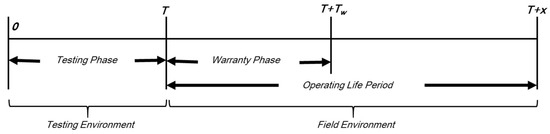
Figure 1. System cost model infrastructure.

The expected total software cost $\mathrm{C}\left(\mathrm{T}\right)$ [24] can be expressed as

$$\mathrm{C}\left(\mathrm{T}\right)={\mathrm{C}}_0+{\mathrm{C}}_1\mathrm{T}+{\mathrm{C}}_2\mathrm{m}\left(\mathrm{T}\right){\mathsf{\mu }}_{\mathrm{y}}+{\mathrm{C}}_3\left(1-\mathrm{R}\left(\mathrm{x}|\mathrm{T}\right)\right)+{\mathrm{C}}_4\left[\mathrm{m}\left(\mathrm{T}+{\mathrm{T}}_{\mathrm{w}}\right)-\mathrm{m}\left(\mathrm{T}\right)\right]{\mathsf{\mu }}_{\mathrm{w}}$$

(17)

where, ${\mathrm{C}}_0$ is the set-up cost of testing, ${\mathrm{C}}_1\mathrm{T}$ is the cost of testing, ${\mathrm{C}}_2\mathrm{m}\left(\mathrm{T}\right){\mathsf{\mu }}_{\mathrm{y}}$ is the expected cost to remove all errors detected by time $\mathrm{T}$ during the testing phase, ${\mathrm{C}}_3\left(1-\mathrm{R}\left(\mathrm{x}|\mathrm{T}\right)\right)$ is the penalty cost owing to failures that occurs after the system release time $\mathrm{T}$, and ${\mathrm{C}}_4\left[\mathrm{m}\left(\mathrm{T}+{\mathrm{T}}_{\mathrm{w}}\right)-\mathrm{m}\left(\mathrm{T}\right)\right]{\mathsf{\mu }}_{\mathrm{w}}$ is the expected cost to remove all of the errors that are detected during the warranty period [$\mathrm{T},\mathrm{T}+{\mathrm{T}}_{\mathrm{w}}$]. The cost that is required to remove faults during the operating period is higher than during the testing period, and the time that is needed is much longer.

Finally, we aim to find the optimal software release time, T*, with the expected minimum in the environment as follows:

$$\mathrm{Minimize}\mathrm{C}\left(\mathrm{T}\right).$$

(18)

5. Numerical Examples

5.1. Data Information

Dataset #1 (DS1), presented in Table 2, was reported by Musa [25] based on software failure data from a real time command and control system (RTC&CS), and represents the failures that were observed during system testing (25 hours of CPU time). The number of test object instructions delivered for this system, which was developed by Bell Laboratories, was 21,700.

Table 2. Dataset #1 (DS1) : real time command and control system (RTC&CS) data set.

Hour Index	Failures	Cumulative Failures	Hour Index	Failures	Cumulative Failures
1	27	27	14	5	111
2	16	43	15	5	116
3	11	54	16	6	122
4	10	64	17	0	122
5	11	75	18	5	127
6	7	83	19	1	128
7	2	84	20	1	129
8	5	89	21	2	131
9	3	92	22	1	132
10	1	93	23	2	134
11	4	97	24	1	135
12	7	104	25	1	136
13	2	106	-	-	-

Dataset #2 (DS2), as shown in Table 3, is the second of three releases of software failure data collected from three different releases of a large medical record system (MRS) [26], consisting of 188 software components. Each component contains several files. Initially, the software consisted of 173 software components. All three releases added new functionality to the product. Between three and seven new components were added in each of the three releases, for a total of 15 new components. Many other components were modified during each of the three releases as a side effect of the added functionality. Detailed information of the dataset can be obtained in the report by Stringfellow and Andrews [26].

Table 3. DS2 : medical record system (MRS) data set.

Week Index	Failures	Cumulative Failures	Week Index	Failures	Cumulative Failures
1	90	90	10	0	190
2	17	107	11	2	192
3	19	126	12	0	192
4	19	145	13	0	192
5	26	171	14	0	192
6	17	188	15	11	203
7	1	189	16	0	203
8	1	190	17	1	204
9	0	190	-	-	-

Dataset #3 (DS3), as shown in Table 4, is from one of four major releases of software products at Tandom Computers (TDC) [27]. There are 100 failures that are observed within testing CPU hours. Detailed information of the dataset can be obtained tin the report by Wood [27].

Table 4. DS3 : Tandom Computers (TDC) data set.

Time Index (CPU hours)	Cumulative Failures	Time Index (CPU hours)	Cumulative Failures	Time Index (CPU hours)	Cumulative Failures
519	16	4422	58	8205	96
968	24	5218	69	8564	98
1430	27	5823	75	8923	99
1893	33	6539	81	9282	100
2490	41	7083	86	9641	100
3058	49	7487	90	10,000	100
3625	54	7846	93	-	-

5.2. Model Analysis

Table 5, Table 6 and Table 7 summarize the results of the estimated parameters of all 10 models in Table 1 using the LSE technique and the values of the six common criteria: MSE, AIC, PRR, PP, SAE, and ${\mathrm{R}}^2$. We obtained the six common criteria at $\mathrm{t}=1,2,\cdots ,25$ from DS1 (Table 2), at $\mathrm{t}=1,2,\cdots ,17$ from DS2 (Table 3), and at cumulative testing CPU hours from DS3 (Table 4). As can be seen in Table 5, when comparing all of the models, the MSE and AIC values are the lowest for the newly proposed model, and the PRR, PP, SAE, and ${\mathrm{R}}^2$ values are the second best. The MSE and AIC values of the newly proposed model are 7.361, 114.982, respectively, which are significantly less than the values of the other models. In Table 6, when comparing all of the models, all criteria values for the newly proposed model are best. The MSE value of the newly proposed model is 60.623, which is significantly lower than the value of the other models. The AIC, PRR, PP, and SAE values of the newly proposed model are 151.156, 0.043, 0.041, and 98.705, respectively, which are also significantly lower than the other models. The value of R² is 0.960 and is the closest to 1 for all of the models. In Table 7, when comparing all of the models, all the criteria values for the newly proposed model are best. The MSE value of the newly proposed model is 6.336, which is significantly lower than the value of the other models. The PRR, PP, and SAE values of the newly proposed model are 0.086, 0.066, and 36.250, respectively, which are also significantly lower than the other models. The value of R² is 0.9940 and is the closest to 1 for all of the models.

Table 5. Model parameter estimation and comparison criteria from RTC&CS data set (DS1). Least-squares estimate (LSE); mean squared error; Akaike’s information criterion (AIC); predictive ratio risk (PRR); predictive power (PP), sum absolute error (SAE), correlation index of the regression curve equation (${\mathrm{R}}^2$ ).

Model	LSE’s	MSE	AIC	PRR	PP	SAE	R2
GOM	$\widehat{\mathrm{a}}$ = 136.050, $\hat{\mathrm{b}}$ = 0.138	33.822	121.878	0.479	0.262	118.530	0.972
DSM	$\hat{\mathrm{a}}$ = 124.665, $\widehat{\mathrm{b}}$ = 0.356	134.582	210.287	12.787	1.181	239.335	0.889
ISM	$\hat{\mathrm{a}}$ = 136.050, $\hat{\mathrm{b}}$ = 0.138 $\hat{\mathsf{\beta }}$ = 0.0001	35.363	123.878	0.479	0.262	118.532	0.972
YIDM	$\widehat{\mathrm{a}}$ = 81.252, $\hat{\mathrm{b}}$ = 0.340 $\hat{\mathsf{\alpha }}$ = 0.0333	9.435	116.403	0.035	0.031	60.842	0.993
PNZM	$\widehat{\mathrm{a}}$ = 81.562, $\widehat{\mathrm{b}}$ = 0.337 $\hat{\mathsf{\alpha }}$ = 0.033, $\hat{\mathsf{\beta }}$ = 0.00	9.888	118.388	0.037	0.032	60.877	0.993
PZM	$\hat{\mathrm{a}}$ = 0.01, $\hat{\mathrm{b}}$ = 0.138 $\widehat{\mathsf{\alpha }}$ = 800.0, $\widehat{\mathsf{\beta }}$ = 0.00, $\widehat{\mathrm{c}}$ = 136.04	38.895	127.878	0.479	0.262	118.530	0.972
DPM	$\hat{\mathsf{\alpha }}$ = 28650, $\hat{\mathsf{\beta }}$ = 0.003 ${\mathrm{t}}_0$ = 0.00, ${\mathrm{m}}_0$ = 71.8	274.911	382.143	0.857	3.568	304.212	0.792
TCM	$\hat{\mathrm{a}}$ = 0.000035, $\widehat{\mathrm{b}}$ = 0.734, $\widehat{\mathsf{\alpha }}$ = 0.29, $\widehat{\mathsf{\beta }}$ = 0.002, $\widehat{\mathrm{N}}$ = 427	7.640	116.932	0.019	0.019	47.304	0.995
3PFDM	$\hat{\mathrm{a}}$ = 1.696, $\widehat{\mathrm{b}}$ = 0.001 $\hat{\mathrm{c}}$ = 6.808, $\hat{\mathsf{\beta }}$ = 1.574 $\widehat{\mathrm{N}}$ = 173.030	17.827	119.523	0.137	0.100	81.313	0.987
New Model	$\widehat{\mathrm{a}}$ = 0.277, $\widehat{\mathsf{\alpha }}$ = 0.328 $\widehat{\mathsf{\beta }}$ = 17.839, $\widehat{\mathrm{N}}$ = 228.909	7.361	114.982	0.022	0.022	47.869	0.994

Table 6. Model parameter estimation and comparison criteria from MRS data set (DS2).

Model	LSE’s	MSE	AIC	PRR	PP	SAE	R2
GOM	$\hat{\mathrm{a}}$ = 197.387, $\widehat{\mathrm{b}}$ = 0.399	80.678	184.331	0.170	0.101	104.403	0.939
DSM	$\hat{\mathrm{a}}$ = 192.528, $\hat{\mathrm{b}}$ = 0.882	232.628	331.857	1.291	0.333	142.544	0.823
ISM	$\hat{\mathrm{a}}$ = 197.354, $\hat{\mathrm{b}}$ = 0.399 $\widehat{\mathsf{\beta }}$ = 0.000001	86.440	186.334	0.171	0.101	104.370	0.939
YIDM	$\hat{\mathrm{a}}$ = 182.934, $\hat{\mathrm{b}}$ = 0.464 $\widehat{\mathsf{\alpha }}$ = 0.0071	78.837	157.825	0.128	0.087	100.617	0.944
PNZM	$\widehat{\mathrm{a}}$ = 183.124, $\hat{\mathrm{b}}$ = 0.463 $\hat{\mathsf{\alpha }}$ = 0.007, $\hat{\mathsf{\beta }}$ = 0.00	84.902	159.873	0.128	0.087	100.608	0.944
PZM	$\hat{\mathrm{a}}$ = 195.990, $\widehat{\mathrm{b}}$ =0.3987 $\hat{\mathsf{\alpha }}$ = 1000.00, $\hat{\mathsf{\beta }}$ = 0.00, $\hat{\mathrm{c}}$ = 1.390	100.989	190.332	0.172	0.102	104.354	0.939
DPM	$\widehat{\mathsf{\alpha }}$ = 26124.0, $\widehat{\mathsf{\gamma }}$ = 0.0044 ${\mathrm{t}}_0$ = 0.00, ${\mathrm{m}}_0$ = 147.00	769.282	480.341	0.415	0.712	334.128	0.494
TCM	$\hat{\mathrm{a}}$ = 0.053, $\widehat{\mathrm{b}}$ = 0.774, $\hat{\mathsf{\alpha }}$ = 181.0, $\hat{\mathsf{\beta }}$ = 38.6, $\hat{\mathrm{N}}$ = 204.1	72.283	158.933	0.052	0.048	103.196	0.956
3PFDM	$\hat{\mathrm{a}}$ = 0.028, $\hat{\mathrm{b}}$ = 0.210 $\widehat{\mathrm{c}}$ = 9.924, $\hat{\mathsf{\beta }}$ = 0.005 $\hat{\mathrm{N}}$ = 206.387	81.090	163.797	0.073	0.061	106.341	0.951
New Model	$\hat{\mathrm{a}}$ = 0.008, $\widehat{\mathsf{\alpha }}$ = 0.275, $\widehat{\mathsf{\beta }}$ = 0.001, $\widehat{\mathrm{N}}$ = 207.873	60.623	151.156	0.043	0.041	98.705	0.960

Table 7. Model parameter estimation and comparison criteria from MRS data set (DS3).

Model	LSE’s	MSE	AIC	PRR	PP	SAE	R2
GOM	$\hat{\mathrm{a}}$ = 133.835, $\hat{\mathrm{b}}$ = 0.000146	8.620	86.136	0.556	0.242	42.166	0.991
DSM	$\hat{\mathrm{a}}$ = 101.918, $\widehat{\mathrm{b}}$ = 0.000507	45.783	117.316	22.692	1.318	101.659	0.951
ISM	$\hat{\mathrm{a}}$ = 133.835, $\widehat{\mathrm{b}}$ = 0.000146 $\hat{\mathsf{\beta }}$ = 0.000001	9.127	88.136	0.556	0.242	42.166	0.991
YIDM	$\hat{\mathrm{a}}$ = 130.091, $\widehat{\mathrm{b}}$ = 0.00015 $\hat{\mathsf{\alpha }}$ = 0.000003	9.084	88.267	0.561	0.243	42.052	0.991
PNZM	$\widehat{\mathrm{a}}$ = 121.178, $\hat{\mathrm{b}}$ = 0.000163 $\hat{\mathsf{\alpha }}$ = 0.000009, $\widehat{\mathsf{\beta }}$ = 0.00	9.532	90.326	0.530	0.234	41.538	0.991
PZM	$\widehat{\mathrm{a}}$ = 122.259, $$ = 0.0002 $\hat{\mathsf{\alpha }}$ = 9955.597, $\hat{\mathsf{\beta }}$ = 0.305 $\widehat{\mathrm{c}}$ = 0.569	11.491	92.020	0.643	0.268	44.848	0.990
DPM	$\hat{\mathsf{\alpha }}$ = 123.193, $\hat{\mathsf{\gamma }}$ = 0.0001 ${\mathrm{t}}_0$ = 0.0001, ${\mathrm{m}}_0$ = 38.459	156.480	212.867	0.917	2.879	196.360	0.851
TCM	$\hat{\mathrm{a}}$ = 0.000013, $\hat{\mathrm{b}}$ = 0.78, $\hat{\mathsf{\alpha }}$ = 141.399, $\widehat{\mathsf{\beta }}$ = 54.71, $\widehat{\mathrm{N}}$ = 254.707	7.090	90.758	0.091	0.068	37.880	0.9937
3PFDM	$\hat{\mathrm{a}}$ = 0.016, $\widehat{\mathrm{b}}$ = 0.07 $\widehat{\mathrm{c}}$ = 0.00001, $\widehat{\mathsf{\beta }}$ = 157.458 $\widehat{\mathrm{N}}$ = 205.025	9.410	92.360	0.420	0.200	39.909	0.992
New Model	$\hat{\mathrm{a}}$ = 0.064, $\hat{\mathsf{\alpha }}$ = 0.731, $\widehat{\mathsf{\beta }}$ = 2509.898, $\widehat{\mathrm{N}}$ = 337.765	6.336	88.885	0.086	0.066	36.250	0.9940

Figure 2, Figure 3 and Figure 4 show the graphs of the mean value functions for all 10 models for DS1, DS2, and DS3, respectively. Figure 5, Figure 6 and Figure 7 show the graphs of the 95% confidence limits of the newly proposed model for DS1, DS2, and DS3. Table A1, Table A2 and Table A3 in Appendix A list the 95% confidence intervals of all 10 NHPP software reliability models for DS1, DS2, and DS3. In addition, the relative error value of the proposed software reliability model confirms its ability to provide more accurate predictions as it remains closer to zero when compared to the other models (Figure 8, Figure 9 and Figure 10).

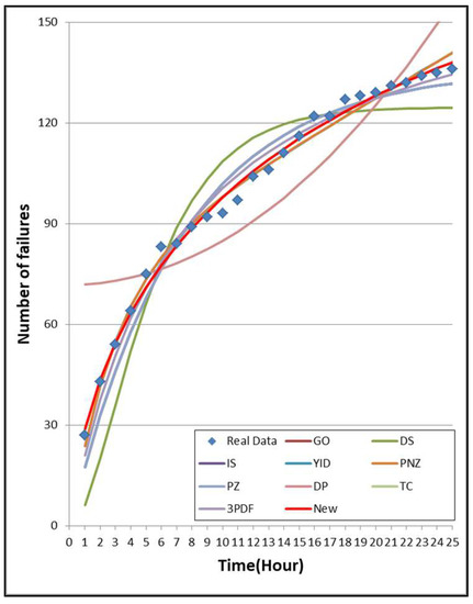
Figure 2. Mean value function of the ten models for DS1.

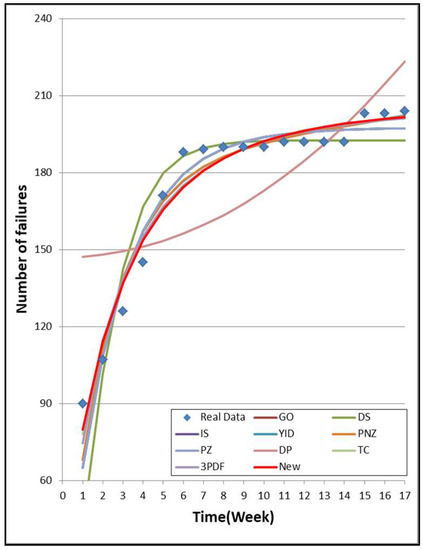
Figure 3. Mean value function of the ten models for DS2.

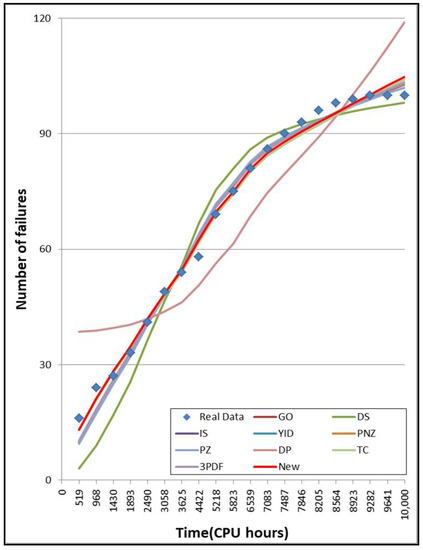
Figure 4. Mean value function of the ten models for DS3.

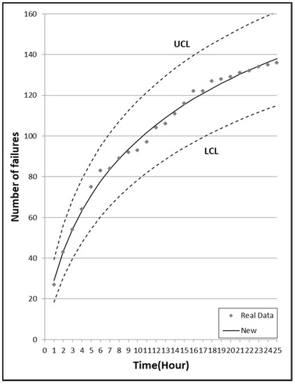
Figure 5. 95% confidence limits of the newly proposed model for DS1.

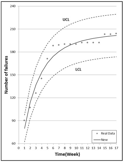
Figure 6. 95% confidence limits of the newly proposed model for DS2.

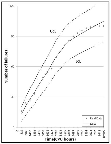
Figure 7. 95% confidence limits of the newly proposed model for DS3.

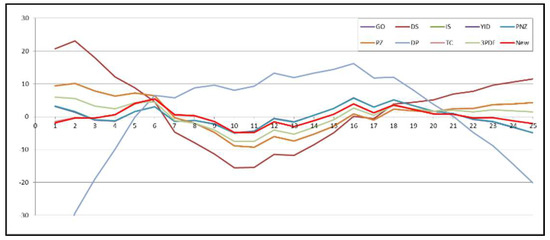
Figure 8. Relative error of the ten models for DS1.

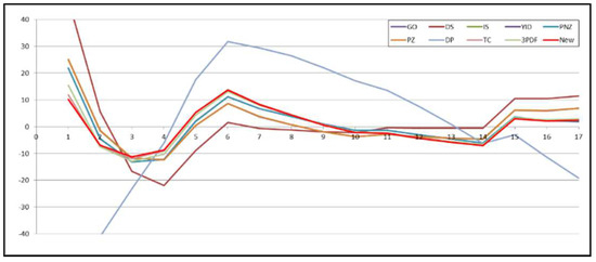
Figure 9. Relative error of the ten models for DS2.

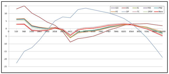
Figure 10. Relative error of the ten models for DS3.

5.3. Optimal Software Release Time

Factor η captures the effects of the field environmental factors based on the system failure rate as described in Section 2. System testing is commonly carried out in a controlled environment, where we can use a constant factor η equal to 1. The newly proposed model becomes a delayed S-shaped model when η = 1 in (7). Thus, we apply different mean value functions $\mathrm{m}\left(\mathrm{t}\right)$ to the cost model $\mathrm{C}\left(\mathrm{T}\right)$ of (8) when considering the three conditions described below. We apply the cost model to these three conditions using DS1 (Table 2). Using the LSE method, the parameters of the delayed S-shaped model and the newly proposed model are obtained, as described in Section 5.2.

(1) The expected total software cost with controlled environmental factor (η = 1) is

$${\mathrm{C}}_1\left(\mathrm{T}\right)={\mathrm{C}}_0+{\mathrm{C}}_1\mathrm{T}+{\mathrm{C}}_2\mathrm{m}\left(\mathrm{T}\right){\mathsf{\mu }}_{\mathrm{y}}+{\mathrm{C}}_3\left(1-\mathrm{R}\left(\mathrm{x}|\mathrm{T}\right)\right)+{\mathrm{C}}_4\left[\mathrm{m}\left(\mathrm{T}+{\mathrm{T}}_{\mathrm{w}}\right)-\mathrm{m}\left(\mathrm{T}\right)\right]{\mathsf{\mu }}_{\mathrm{w}}$$

(19)

where

$$\mathrm{m}\left(\mathrm{T}\right)=\mathrm{a}(1-\left(1+\mathrm{bT}\right){\mathrm{e}}^{-\mathrm{bT}}),\mathrm{m}\left(\mathrm{T}+{\mathrm{T}}_{\mathrm{w}}\right)=\mathrm{a}(1-\left(1+\mathrm{b}\left(\mathrm{T}+{\mathrm{T}}_{\mathrm{w}}\right)\right){\mathrm{e}}^{-\mathrm{b}\left(\mathrm{T}+{\mathrm{T}}_{\mathrm{w}}\right)}).$$

(20)

(2) The expected total software cost with a random operating environmental factor (η = f(x)) is

$${\mathrm{C}}_2\left(\mathrm{T}\right)={\mathrm{C}}_0+{\mathrm{C}}_1\mathrm{T}+{\mathrm{C}}_2\mathrm{m}\left(\mathrm{T}\right){\mathsf{\mu }}_{\mathrm{y}}+{\mathrm{C}}_3\left(1-\mathrm{R}\left(\mathrm{x}|\mathrm{T}\right)\right)+{\mathrm{C}}_4\left[\mathrm{m}\left(\mathrm{T}+{\mathrm{T}}_{\mathrm{w}}\right)-\mathrm{m}\left(\mathrm{T}\right)\right]{\mathsf{\mu }}_{\mathrm{w}}$$

(21)

where

$$\mathrm{m}\left(\mathrm{T}\right)=\mathrm{N}{\left(1-\frac{\mathsf{\beta }}{\mathsf{\beta }+\mathrm{aT}-\ln \left(1+\mathrm{aT}\right)}\right)}^{\mathsf{\alpha }},\mathrm{m}\left(\mathrm{T}+{\mathrm{T}}_{\mathrm{w}}\right)=\mathrm{N}{\left(1-\frac{\mathsf{\beta }}{\mathsf{\beta }+\mathrm{a}\left(\mathrm{T}+{\mathrm{T}}_{\mathrm{w}}\right)-\ln \left(1+\mathrm{a}\left(\mathrm{T}+{\mathrm{T}}_{\mathrm{w}}\right)\right)}\right)}^{\mathsf{\alpha }}.$$

(22)

(3) The expected total software cost between the testing environment (η = 1) and field environment (η = f(x)) is

$${\mathrm{C}}_3\left(\mathrm{T}\right)={\mathrm{C}}_0+{\mathrm{C}}_1\mathrm{T}+{\mathrm{C}}_2{\mathrm{m}}_1\left(\mathrm{T}\right){\mathsf{\mu }}_{\mathrm{y}}+{\mathrm{C}}_3\left(1-\mathrm{R}\left(\mathrm{x}|\mathrm{T}\right)\right)+{\mathrm{C}}_4\left[{\mathrm{m}}_2\left(\mathrm{T}+{\mathrm{T}}_{\mathrm{w}}\right)-{\mathrm{m}}_1\left(\mathrm{T}\right)\right]{\mathsf{\mu }}_{\mathrm{w}}$$

(23)

where

$${\mathrm{m}}_1\left(\mathrm{T}\right)=\mathrm{a}\left(1-\left(1+\mathrm{bT}\right){\mathrm{e}}^{-\mathrm{bT}}\right),{\mathrm{m}}_2\left(\mathrm{T}+{\mathrm{T}}_{\mathrm{w}}\right)=\mathrm{N}{\left(1-\frac{\mathsf{\beta }}{\mathsf{\beta }+\mathrm{a}\left(\mathrm{T}+{\mathrm{T}}_{\mathrm{w}}\right)-\ln \left(1+\mathrm{a}\left(\mathrm{T}+{\mathrm{T}}_{\mathrm{w}}\right)\right)}\right)}^{\mathsf{\alpha }}.$$

(24)

We consider the following coefficients in the cost model for the baseline case:

$${\mathrm{C}}_0=100,{\mathrm{C}}_1=20,{\mathrm{C}}_2=50,{\mathrm{C}}_3=2000,{\mathrm{C}}_4=400,{\mathrm{T}}_{\mathrm{w}}=10,\mathrm{x}=20,{\mathsf{\mu }}_{\mathrm{y}}=0.1,{\mathsf{\mu }}_{\mathrm{w}}=0.2$$

(25)

The results of the baseline case are listed in Table 8, and the expected total cost for the three conditions above is 1338.70, 2398.24, and 2263.33, respectively. For the second condition, the expected total cost and the optimal release time are high. The expected total cost is the lowest for the first condition, and the optimal release time is shortest for the third condition.

Table 8. Optimal release time T* subject to the warranty period.

Warrnaty Period	C1(T)	T*	C2(T)	T*	C3(T)	T*
Tw = 2	1173.41	14.2	1403.78	11.6	599.88	10.5
Tw = 5	1286.95	14.9	1928.63	22.8	1334.72	11.3
Tw = 10(basic)	1338.70	15.1	2398.24	34.7	2263.33	12.3
Tw = 15	1348.88	15.2	2702.33	42.7	2969.88	13.0

To study the impact of different coefficients on the expected total cost and the optimal release time, we vary some of the coefficients and then compare them with the baseline case. First, we evaluate the impact of the warranty period on the expected total cost by changing the value of the corresponding warranty time and comparing the optimal release times for each condition. Here, we change the values of T_w from 10 h to 2, 5, and 15 h, and the values of the other parameters remain unchanged. Regardless of the warranty period, the optimal release time for the third condition is the shortest, and the expected total cost for the first condition is the lowest overall. Figure 11 shows the graph of the expected total cost for the baseline case. Figure 12, Figure 13 and Figure 14 show the graphs of the expected total cost subject to the warranty period for the three conditions.

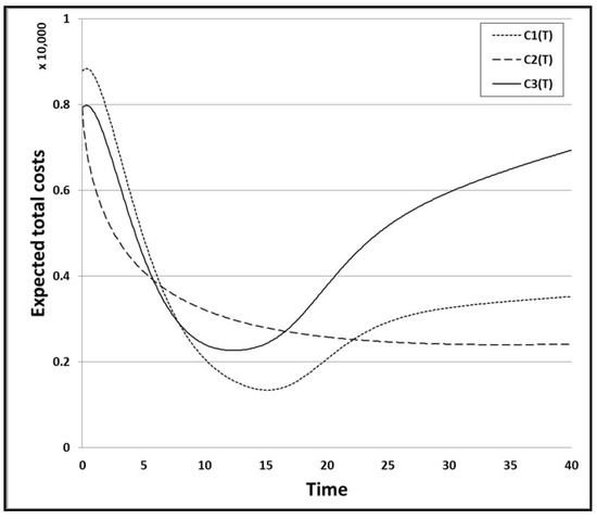
Figure 11. Expected total cost for the baseline case.

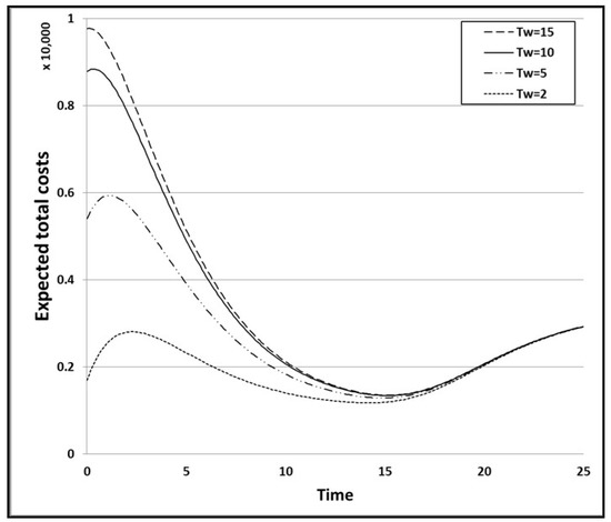
Figure 12. Expected total cost subject to the warranty period for the 1st condition.

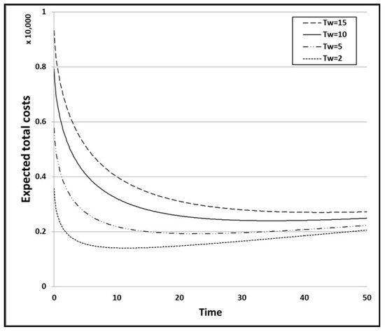
Figure 13. Expected total cost subject to the warranty period for the 2nd condition.

Figure 14. Expected total cost subject to the warranty period for the 3rd condition.

Next, we examine the impact of the cost coefficients, C₁, C₂, C₃, and C₄ on the expected total cost by changing their values and comparing the optimal release times. Without loss of generality, we change only the values of C₂, C₃, and C₄, and keep the values of the other parameters C₀ and C₁ unchanged, because different values of C₀ and C₁ will certainly increase the expected total cost. When we change the values of C₂ from 50 to 25 and 100, the optimal release time is only changed significantly for the second condition. As can be seen from Table 9, the optimal release time T* is 37.5 when the value of C₂ is 25, and 29.1 when the value of C₂ is 100. When we change the value of C₃ from 2000 to 500 and 4000, the optimal release time is only changed significantly for the first condition. As Table 10 shows, the optimal release time T* is 16.5 when the value of C₃ is 500, and 14.6 when the value of C₃ is 4000. When we change the value of C₄ from 400 to 200 and 1000, the optimal release time is changed for all of the conditions. As can be seen from Table 11, the optimal release time T* is 14.3 for the first condition when the value of C₄ is 200, and 16.3 when the value of C₄ is 1000. In addition, the optimal release time T* is 20.0 for the second condition when the value of C₄ is 200, and 61.0 when the value of C₄ is 1000. The optimal release time T* is 11.6 for the third condition when the value of C₄ is 200, and 12.8 when the value of C₄ is 1000. Thus, the second condition has a much greater variation in optimal release time than the other conditions. As a result, we can confirm that the cost model of the first condition does not reflect the influence of the operating environment, and that the cost model of the second condition does not reflect the influence of the test environment. Figure 15 shows the graph of the expected total cost according to the cost coefficient C₂ in the 2nd condition. Figure 16, Figure 17 and Figure 18 show the graphs of the expected total cost according to cost coefficient C₄ in the three conditions.

Table 9. Optimal release time T* according to cost coefficient C_2.

Cost Coefficient C2	C1(T)	T*	C2(T)	T*	C3(T)	T*
C2 = 25	1036.02	15.2	2013.25	37.5	1972.06	12.5
C2 = 50 (basic)	1338.70	15.1	2398.24	34.7	2263.33	12.3
C2 = 100	1943.64	15.1	3141.20	29.1	2843.35	12.1

Table 10. Optimal release time T* according to cost coefficient C_3.

Cost Coefficient C3	C1(T)	T*	C2(T)	T*	C3(T)	T*
C3 = 500	1270.65	16.5	2398.24	34.7	2262.96	12.4
C3 = 2000 (basic)	1338.70	15.1	2398.24	34.7	2263.33	12.3
C3 = 4000	1376.26	14.6	2398.24	34.7	2263.77	12.3

Table 11. Optimal release time T* according to cost coefficient C_4.

Cost Coefficient C4	C1(T)	T*	C2(T)	T*	C3(T)	T*
C4 = 200	1183.14	14.3	1859.29	20	1590.02	11.6
C4 = 400 (basic)	1338.70	15.1	2398.24	34.7	2263.33	12.3
C4 = 1000	1680.99	16.3	3272.23	61	4253.45	12.8

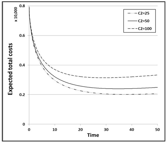
Figure 15. Expected total cost according to cost coefficient C₂ for the 2nd condition.

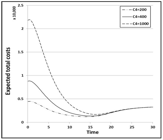
Figure 16. Expected total cost according to cost coefficient C₄ for the 1st condition.

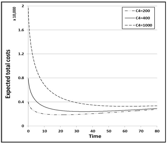
Figure 17. Expected total cost according to cost coefficient C₄ for the 2nd condition.

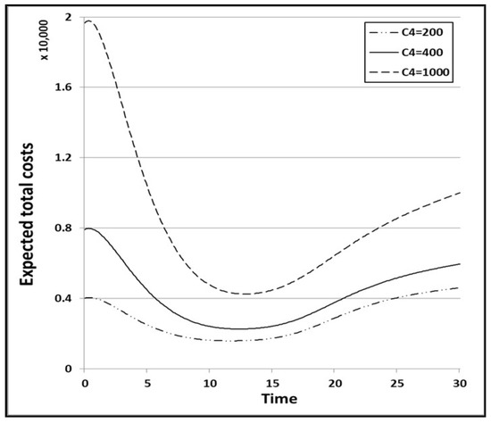
Figure 18. Expected total cost according to cost coefficient C₄ for the 3rd condition.

6. Conclusions

Existing well-known NHPP software reliability models have been developed in a test environment. However, a testing environment differs from an actual operating environment, so we considered random operating environments. In this paper, we discussed a new NHPP software reliability model, with S-shaped growth curve that accounts for the randomness of an actual operating environment. Table 5, Table 6 and Table 7 summarize the results of the estimated parameters of all ten models that are applied using the LSE technique and six common criteria (MSE, AIC, PRR, PP, SAE, and R²) for the DS1, DS2, and DS3 datasets. As can be seen from Table 5, Table 6 and Table 7, the newly proposed model displays a better overall fit than all of the other models when compared, particularly in the case of DS2. In addition, we provided optimal release policies for various environments to determine when the total software system cost is minimized. Using a cost model for a given environment is beneficial as it provides a means for determining when to stop the software testing process. In this paper, faults are assumed to be removed immediately when a software failure has been detected, and the correction process is assumed to not introduce new faults. Obviously, further work in revisiting these assumptions is worth the effort as our future study. We hope to present some new results on this aspect in the near future.

References

- Pham, T.; Pham, H. A generalized software reliability model with stochastic fault-detection rate. Ann. Oper. Res. 2017, 1–11. [Google Scholar] [CrossRef]
- Teng, X.; Pham, H. A new methodology for predicting software reliability in the random field environments. IEEE Trans. Reliab. 2006, 55, 458–468. [Google Scholar] [CrossRef]
- Pham, H. A new software reliability model with Vtub-Shaped fault detection rate and the uncertainty of operating environments. Optimization 2014, 63, 1481–1490. [Google Scholar] [CrossRef]
- Chang, I.H.; Pham, H.; Lee, S.W.; Song, K.Y. A testing-coverage software reliability model with the uncertainty of operation environments. Int. J. Syst. Sci. Oper. Logist. 2014, 1, 220–227. [Google Scholar]
- Inoue, S.; Ikeda, J.; Yamada, S. Bivariate change-point modeling for software reliability assessment with uncertainty of testing-environment factor. Ann. Oper. Res. 2016, 244, 209–220. [Google Scholar] [CrossRef]
- Okamura, H.; Dohi, T. Phase-type software reliability model: Parameter estimation algorithms with grouped data. Ann. Oper. Res. 2016, 244, 177–208. [Google Scholar] [CrossRef]
- Song, K.Y.; Chang, I.H.; Pham, H. A Three-parameter fault-detection software reliability model with the uncertainty of operating environments. J. Syst. Sci. Syst. Eng. 2017, 26, 121–132. [Google Scholar] [CrossRef]
- Song, K.Y.; Chang, I.H.; Pham, H. A software reliability model with a Weibull fault detection rate function subject to operating environments. Appl. Sci. 2017, 7, 983. [Google Scholar] [CrossRef]
- Li, Q.; Pham, H. NHPP software reliability model considering the uncertainty of operating environments with imperfect debugging and testing coverage. Appl. Math. Model. 2017, 51, 68–85. [Google Scholar] [CrossRef]
- Pham, H.; Nordmann, L.; Zhang, X. A general imperfect software debugging model with S-shaped fault detection rate. IEEE Trans. Reliab. 1999, 48, 169–175. [Google Scholar] [CrossRef]
- Pham, H. A generalized fault-detection software reliability model subject to random operating environments. Vietnam J. Comput. Sci. 2016, 3, 145–150. [Google Scholar] [CrossRef]
- Akaike, H. A new look at statistical model identification. IEEE Trans. Autom. Control 1974, 19, 716–719. [Google Scholar] [CrossRef]
- Pham, H. System Software Reliability; Springer: London, UK, 2006. [Google Scholar]
- Goel, A.L.; Okumoto, K. Time dependent error detection rate model for software reliability and other performance measures. IEEE Trans. Reliab. 1979, 28, 206–211. [Google Scholar] [CrossRef]
- Yamada, S.; Ohba, M.; Osaki, S. S-shaped reliability growth modeling for software fault detection. IEEE Trans. Reliab. 1983, 32, 475–484. [Google Scholar] [CrossRef]
- Ohba, M. Inflexion S-shaped software reliability growth models. In Stochastic Models in Reliability Theory; Osaki, S., Hatoyama, Y., Eds.; Springer: Berlin, Germany, 1984; pp. 144–162. [Google Scholar]
- Yamada, S.; Tokuno, K.; Osaki, S. Imperfect debugging models with fault introduction rate for software reliability assessment. Int. J. Syst. Sci. 1992, 23, 2241–2252. [Google Scholar] [CrossRef]
- Pham, H.; Zhang, X. An NHPP software reliability models and its comparison. Int. J. Reliab. Qual. Saf. Eng. 1997, 4, 269–282. [Google Scholar] [CrossRef]
- Pham, H. Software Reliability Models with Time Dependent Hazard Function Based on Bayesian Approach. Int. J. Autom. Comput. 2007, 4, 325–328. [Google Scholar] [CrossRef]
- Li, X.; Xie, M.; Ng, S.H. Sensitivity analysis of release time of software reliability models incorporating testing effort with multiple change-points. Appl. Math. Model. 2010, 34, 3560–3570. [Google Scholar] [CrossRef]
- Pham, H. Software reliability and cost models: Perspectives, comparison, and practice. Eur. J. Oper. Res. 2003, 149, 475–489. [Google Scholar] [CrossRef]
- Pham, H.; Zhang, X. NHPP software reliability and cost models with testing coverage. Eur. J. Oper. Res. 2003, 145, 443–454. [Google Scholar] [CrossRef]
- Kimura, M.; Toyota, T.; Yamada, S. Economic analysis of software release problems with warranty cost and reliability requirement. Reliab. Eng. Syst. Saf. 1999, 66, 49–55. [Google Scholar] [CrossRef]
- Sgarbossa, F.; Pham, H. A cost analysis of systems subject to random field environments and reliability. IEEE Trans. Syst. Man Cybern. Part C Appl. Rev. 2010, 40, 429–437. [Google Scholar] [CrossRef]
- Musa, J.D.; Iannino, A.; Okumoto, K. Software Reliability: Measurement, Prediction, and Application; McGraw-Hill: New York, NY, USA, 1987. [Google Scholar]
- Stringfellow, C.; Andrews, A.A. An empirical method for selecting software reliability growth models. Empir. Softw. Eng. 2002, 7, 319–343. [Google Scholar] [CrossRef]
- Wood, A. Predicting software reliability. IEEE Comput. Soc. 1996, 11, 69–77. [Google Scholar] [CrossRef]
© 2017 by the authors. Licensee MDPI, Basel, Switzerland. This article is an open access article distributed under the terms and conditions of the Creative Commons Attribution (CC BY) license (http://creativecommons.org/licenses/by/4.0/).