Compact Aberration-Free Relay-Imaging Multi-Pass Layouts for High-Energy Laser Amplifiers

Abstract

We present the results from a theoretical investigation of laser beam propagation in relay imaging multi-pass layouts, which recently found application in high-energy laser amplifiers. Using a method based on the well-known ABCD-matrix formalism and proven by ray tracing, it was possible to derive a categorization of such systems. Furthermore, basic rules for the setup of such systems and the compensation for low order aberrations are derived. Due to the introduced generalization and parametrization, the presented results can immediately be applied to any system of the investigated kinds for a wide range of parameters, such as number of round-trips, focal lengths and optics sizes. It is shown that appropriate setups allow a close-to-perfect compensation of defocus caused by a thermal lens and astigmatism caused by non-normal incidence on the imaging optics, as well. Both are important to avoid intensity spikes leading to damages of optics in multi-pass laser amplifiers.

1. Introduction

In the last two decades, the output energy of diode pumped high energy lasers based on Ytterbium doped materials has scaled the achievable output energies into the range of tens of Joules for nanosecond pulses [1], as well as for femtosecond pulses within laser architectures based on the chirped pulse amplification technique [2]. The major advantage of these materials is the long upper state lifetime in comparison to neodymium-doped materials, which are widely used in flash-lamp pumped, high energy systems. This allows one to store a large amount of energy within the active medium with comparably low pump power. Thus, a lower power laser diode pump engine can be used, which reduces size and cost. Nevertheless, this advantage comes at the price of significantly lower cross-sections of the laser medium. Hence, extracting the energy and achieving a reasonable gain in the amplifier requires a higher number of material passes. A major task for the development of such laser systems is the design of multi-pass setups that maintain the typically top-hat-shaped beam profile throughout many amplification steps. As such, beam profiles cannot be propagated without significant diffraction effects, only imaging systems are suitable for this task. In these systems, aberrations should be as little as possible. These includes low order aberrations, as these may cause high intensities, leading to damages of optical elements, clipping of the beam profile due to the deformation of the beam or inhomogeneous depletion of the excitation and, therefore, less efficient amplification.

Though this task is pretty similar to spectroscopic multi-pass cells, the readily available setups, such as Herriott or White cells [3], are no solution for laser amplifiers, since these cells either do not have an image plane that is passed multiple times or as there are non-planar optics within their image planes, which is not feasible in a laser amplifier, since the laser material should be placed in these image planes.

In recent years, some compact imaging multi-pass layouts have been demonstrated. With these setups, a high beam quality and a high number of round-trips have been achieved [4,5,6,7]. Furthermore, due to the repeated use of the imaging optics, the setups described in [5,6,7] allowed one to achieve a high number of material passes with a low number of optics. Such systems offer to scale the number of round-trips without increasing the number of optics, which allows one to achieve simple and compact designs for multi-pass imaging laser amplifiers. Similar layouts with integration into cavities of regenerative amplifiers to achieve multiple amplification passes per resonator round-trip were patented by M. Kumkar et al. [8].

In this work, we will present a method to analyze such systems with multiple round-trips and repeated use of the imaging optics by employing the ABCD-matrix formalism. These imaging elements will be modeled as ideal lenses, while in the following ray tracing simulations, spherical optics will be used for practical reasons.

Thus, starting with only a few basic assumptions, we are able to categorize these systems into two fundamental types. These two kinds of setups are investigated separately for the introduced low order aberrations. First, the defocus, caused by thermal lensing, is investigated. Secondly, astigmatism, caused by tilted incidence on the imaging elements, is analyzed. In both cases, the generalized design parameters and the number of round-trips are varied. We will also derive means for corrections to the system parameters that allow one to compensate for these unwanted effects.

The presented results from the paraxial one-dimensional matrix model are cross-checked using the ray tracing software FRED (Version 9.110 Optimum, Photon Engineering LLC, Tucson, AZ, USA, 2010). Here, an automated routine was programmed to compute the wavefront produced by sample systems with varying parameters. The retrieved wave-fronts were further processed using MATLAB (Version R2012a, MathWorks Inc., Natick, MA, USA, 2012) to obtain the corresponding Zernike coefficients. Using these, a comparison with the parameters calculated with the matrix formalism is realized.

2. The ABCD-Matrix Model

Using the paraxial approximation, any classical optical system containing only translations of lengths d and imaging elements with focal length f can be described by the matrices T for translation and L for the imaging element:

$$\begin{array}{c}\hfill T=\left[\begin{array}{cc}1& d\\ 0& 1\end{array}\right]L=\left[\begin{array}{cc}1& 0\\ -1/f& 1\end{array}\right]\end{array}$$

(1)

In the following, we assume that a round-trip in an imaging multi-pass amplifier is described by alternating free space propagation and ideal imaging elements. Hence, the matrix representing one round-trip in a system of n elements is calculated by:

$$\begin{array}{ccc}\hfill G_n& =& T_{n+1}·L_n·T_n·L_{n-1}·\dots ·L_1·T_1\hfill \end{array}$$

(2)

An imaging system suitable for allowing several round-trips has to restore both the spatial and the angular distribution after each round-trip. Hence, it is required that the optical system matrix equals either the unity matrix U or in the case of a symmetric profile, the negative unity matrix $-U$. If we furthermore demand a constant small angle add-on per pass of the system to separate the different beam passes geometrically, e.g., by introducing a little tilt of the flat optics in the image plane, the latter solution has to be omitted, as the alternating direction of the angular add on will prevent a summation.

Under these constraints, the prescriptions for building such an imaging system can be derived by solving the matrix equation $G_n=U$. In the following, we will give the results for $n=1\dots 3$. Solutions for systems of more than three elements are no longer distinct, as there are too many degrees of freedom. Nevertheless, the used algorithm could be applied for these cases accordingly, especially as most of such systems can be described by a concatenation of systems with less than four imaging elements. In this case, the results presented in the following can be directly applied to the sub-systems.

Starting with a system containing only one imaging element per round-trip, there is no solution, as the focusing or de-focusing effect of the single optic cannot be mitigated and will always alter the collimation state of the input beam.

In the case of $n=2$, there is again no solution that allows one to generate a positive unity matrix. Nevertheless, a solution is found for the negative unity matrix. Hence, double passing such a system back and forth will result in a unity matrix again. This is in a narrower sense a special case for four imaging elements. The solution in this case is:

$$\begin{array}{ccc}\hfill d_1& =& \frac{f_1{f}_2·(f_1+f_2)-d_3{f}_1^2}{f_2^2}\hfill \end{array}$$

(3)

$$\begin{array}{ccc}\hfill d_2& =& f_1+f_2\hfill \end{array}$$

(4)

$$\begin{array}{ccc}\hfill f_1& =& f_2\hfill \end{array}$$

(5)

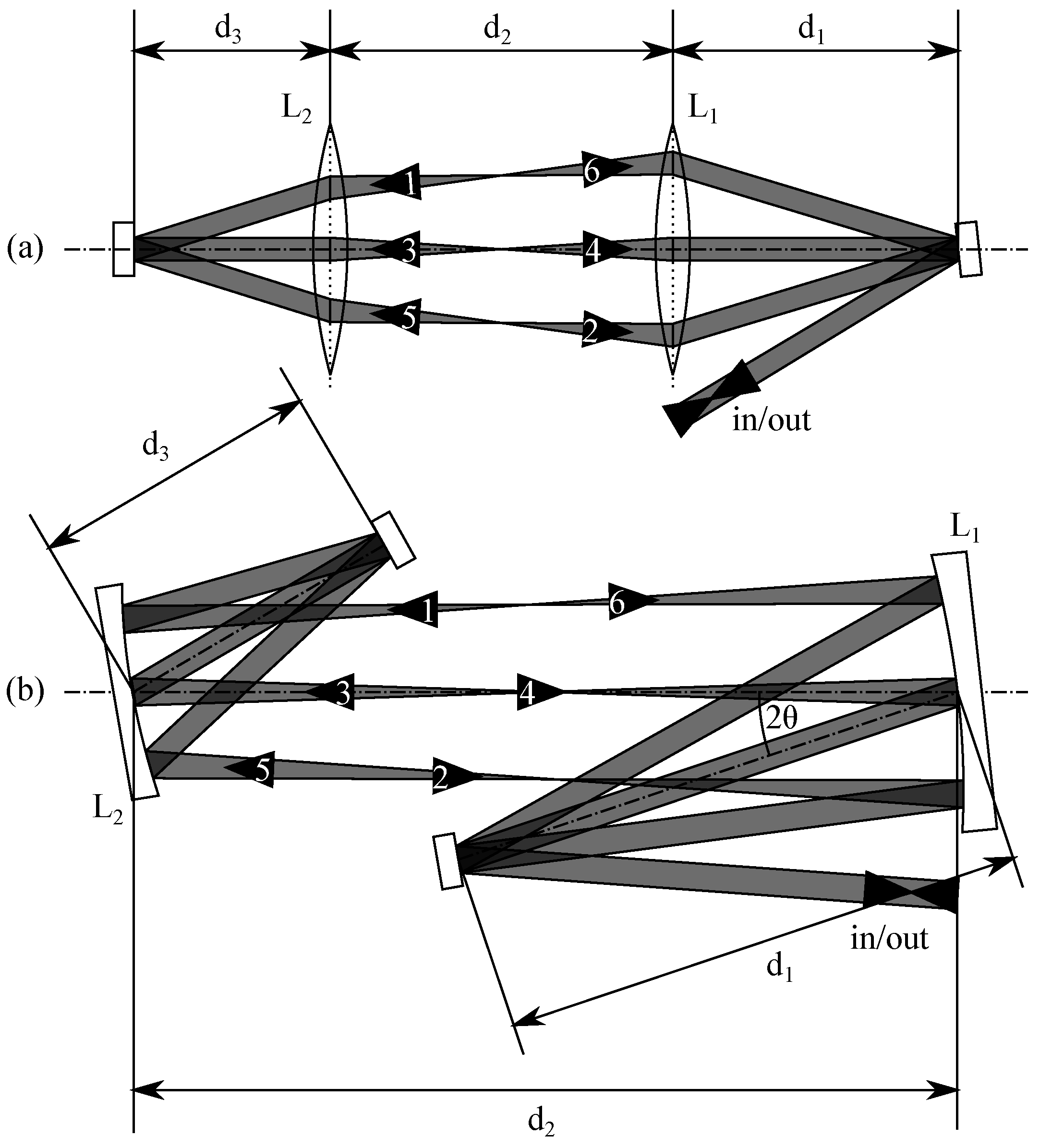
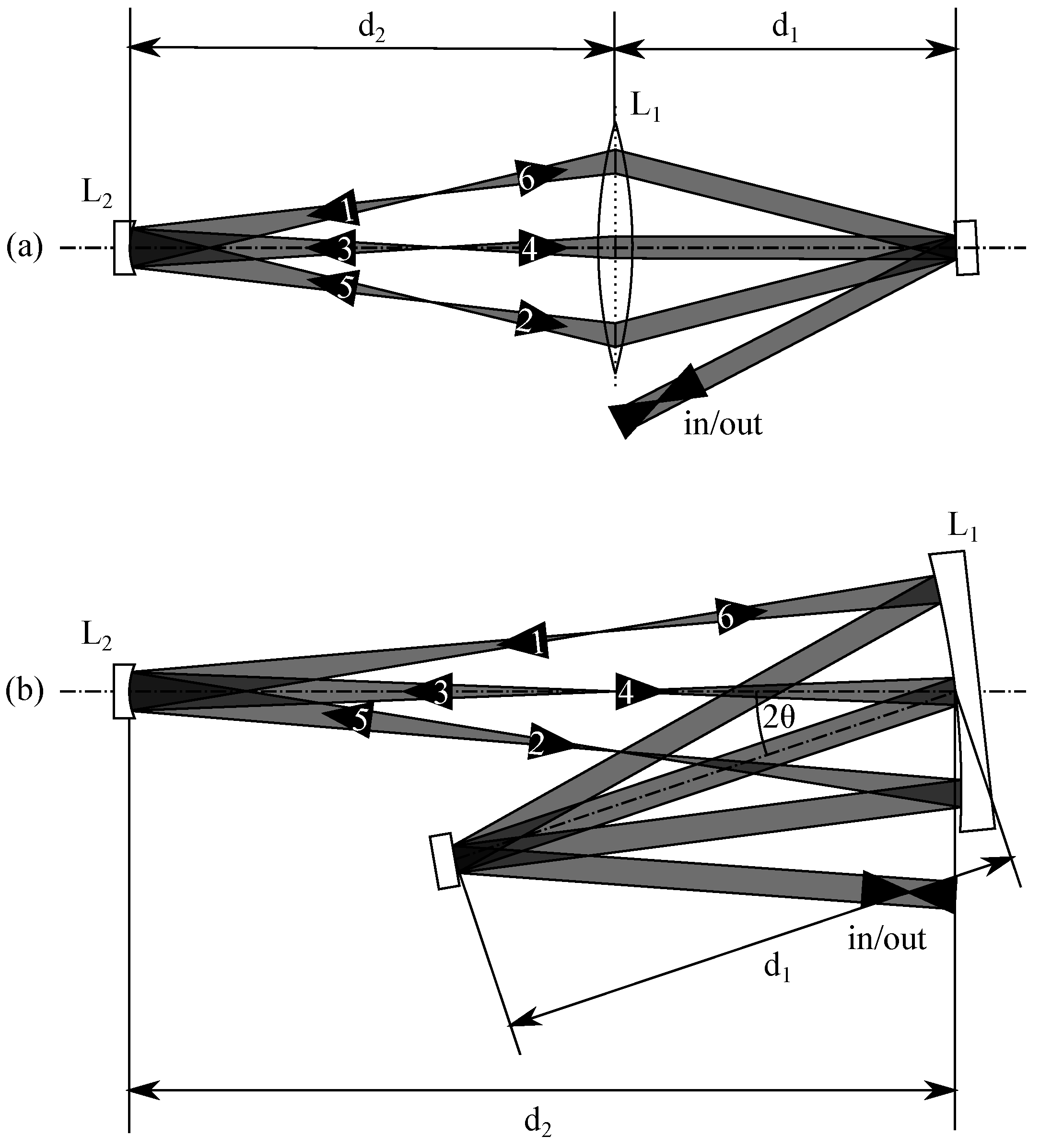
Here, $d_1$ to $d_3$ are the corresponding free space propagation distances, and $f_1$ and $f_2$ are the focal lengths of the imaging elements. This corresponds to the widely-used version of a double-passed 4f-telescope for a multiple imaging layout as, e.g., in [4,6,7]. We will refer to such a kind of system in the following as a Type I system. Schematic setups for optical systems of this type accomplishing three round-trips are exemplarily given in Figure 1.

As this system needs to be double passed to fulfill the constraints, it is not really necessary to have a unity magnification, as was originally requested by the constraints used for deriving this solution. This renders Equation (5) unnecessary, but since all distances have to be ≥0, it follows from Equations (3) and (4) that $f_1$ and $f_2$ must be at least positive. For a system with three imaging elements, there are already too many degrees of freedom with respect to the four different distances to get a closed solution for each distance using our matrix model. Therefore, we concentrate on the special case of a symmetrical system, where the layout is mirrored at the second imaging element. Hence, the additional constraints $f_3=f_1$, $d_4=d_1$ and $d_3=d_2$ reduce the degrees of freedom. Furthermore, in a practical setup, such a layout is very advantageous, as it only requires two different imaging elements. In this case, the ABCD-model results in the following constraints:

$$\begin{array}{ccc}\hfill d_1& =& \frac{f_1^2+2f_1{f}_2}{2f_2}\hfill \end{array}$$

(6)

$$\begin{array}{ccc}\hfill d_2& =& f_1+2f_2\hfill \end{array}$$

(7)

Similar to the Type I system, both $f_1$ and $f_2$ have to be positive to obtain positive distances. Furthermore, solving these results for $\raisebox{1ex}{$1$}\!\left/ \!\raisebox{-1ex}{$f_1$}\right.$, one obtains the imaging equation for an ideal lens:

$$\begin{array}{c}\hfill \frac{1}{f_1}=\frac{1}{d_1}+\frac{1}{d_2}\end{array}$$

(8)

Hence, this system will generate an image of the original beam on the second optical element. This reverses the angular distribution, and the beam is then imaged back to the original image plane by the first element. The diameter of the second element only has to be large enough for supporting the beam itself, as the individual round-trips will not be spatially separated on this optic. Such a system will be referred to as Type II in the following. Schematic examples are given in Figure 2 for three round-trips also.

It should be mentioned that Type I systems are identical to Type II systems for $d_3=0$ and half the focal length of the second element, to consider the double pass on this element. Under these conditions, Equations (3), (4) and (6), (7) are equivalent.

3. Influence of Thermal Lensing and Intrinsic Compensation

In a bulk laser, the thermal load originating from the laser process generates a temperature profile in the laser medium due to thermal expansion and the temperature dependence of the refractive index. This effect is known as thermal lensing. Typically, the most prominent effect is a focusing or defocusing of the beam by the thermal lens leading to increased intensities on amplifier optics and finally to optical damages. This should therefore be considered in the setup.

In the imaging multi-pass schemes presented in this work, the laser active medium is envisioned to be situated in the primary image plane. Hence, due to the imaging properties, the actual beam shape in this plane will be constant irrespective of a thermal lens. Nevertheless, the collimation state will be altered, adding up the focusing of the thermal lens with every round-trip. It is therefore essential to include a means of compensation within the system counteracting this effect. In the following, we will demonstrate that this is possible due to slight adaptions to the optics distances in systems of both types. The thermal lens will be represented by the matrix $L_t$ as an ideal lens with focal length $f_t$.

In a Type I system, this lens is only passed once per half round trip represented by $G_2$. Hence, the modified matrix $G_2^{*}$ is calculated by:

$$\begin{array}{c}\hfill G_2^{*}=G_2·L_t\end{array}$$

(9)

To achieve a compensation in $G_2^{*}$, again, all entries have to be zero, except for the main axis.

The corrected distances are:

$$\begin{array}{c}\hfill d_1=f_1+\frac{f_t}{2}·\left(1-\sqrt{1+\frac{4f_1^2·(d_3-f_2)}{f_t{f}_2^2}}\right)\end{array}$$

(10)

$$\begin{array}{c}\hfill d_2=\frac{f_1{f}_2+(f_1+f_2)·(f_t-d_1)}{f_t+f_1-d_1}\end{array}$$

(11)

$$\begin{array}{c}\hfill d_3=f_2+\frac{f_2^2·(f_1-d_1)}{f_1^2}·\left(1+\frac{f_1-d_1}{f_t}\right)\end{array}$$

(12)

By deriving these compensating solution, all other solutions that do not converge to the original Type I solution for $f_t\to \infty$ are omitted, as these would represent systems integrating the thermal lens as an additional imaging element. A more intuitive formulation of Equations (10)–(12) can be obtained for a standard layout with $d_1=f_1$:

$$\begin{array}{c}\hfill d_1=f_1\end{array}$$

(13)

$$\begin{array}{c}\hfill d_2=f_1+f_2-\frac{f_1^2}{f_t}\end{array}$$

(14)

$$\begin{array}{c}\hfill d_3=f_2\end{array}$$

(15)

According to this solution, the spherical part of a thermal lens in a Type I system can be completely compensated just by adjusting the distance between the imaging optics. In this case, it can further be deduced that the focal length of the thermal lens can only be compensated as long as:

$$\begin{array}{c}\hfill f_t\ge \frac{f_1^2}{f_1+f_2}\end{array}$$

(16)

otherwise, $d_2$ will become negative. However, in real life, setups $f_t$ should be much bigger than $f_1$ in order to avoid intensity spikes on the imaging elements.

The modified matrix for a Type II system, in which the thermal lens is passed in the beginning and at the end of each round-trip, is calculated using:

$$\begin{array}{c}\hfill G_3^{*}=L_t·G_3·L_t\end{array}$$

(17)

To compensate for a thermal lens, $G_3^{*}$ again needs to be equal to U, which leads to:

$$\begin{array}{c}\hfill d_1=f_1+\frac{f_t}{2}·\left(1-\sqrt{1-\frac{2f_1^2}{f_2{f}_t}}\right)\end{array}$$

(18)

$$\begin{array}{c}\hfill d_2=f_1+f_2·\left(1+\sqrt{1-\frac{2f_1^2}{f_2{f}_t}}\right)\end{array}$$

(19)

As for the Type I system, all solutions that do not converge to the original Type II solution for $f_t\to \infty$ are omitted; though the length of both arms is changed. The lens Equation (8) is also valid for the new solution. Hence, the major effect of the thermal lens can be seen as a virtual change of the focal length of $L_2$.

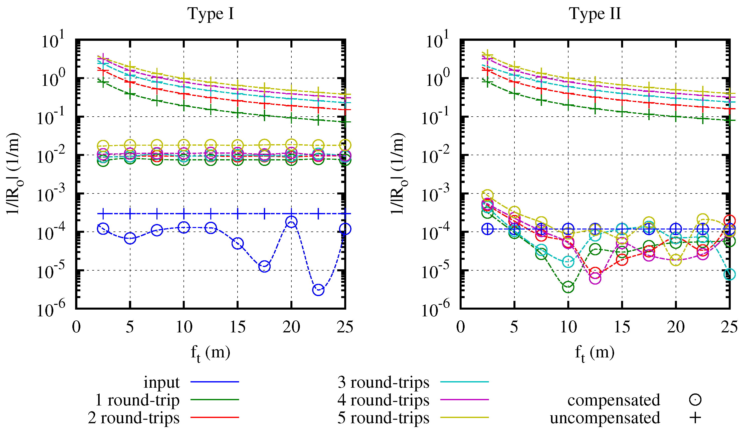
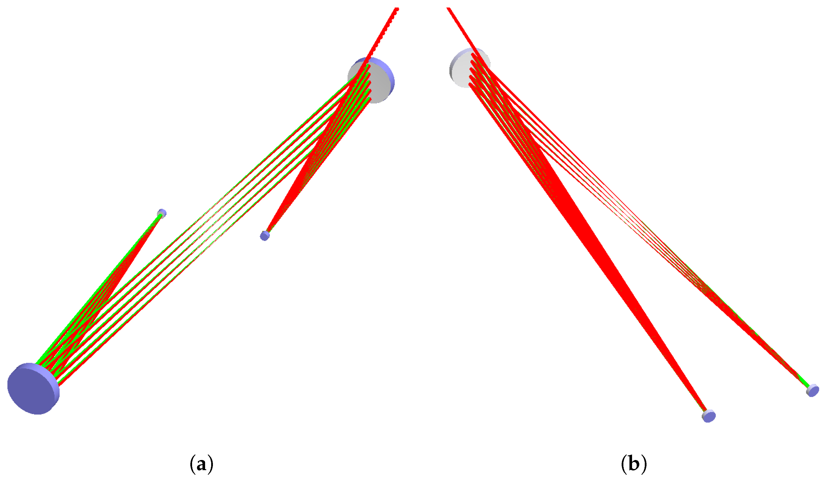
In Figure 3, the validity of the derived compensation formulas is demonstrated using the ray-tracing software FRED. The traces are performed for compensated, as well as for uncompensated systems for different values of $f_t$ and for up to five round-trips. The exact parameters of the test systems are displayed in

Table 1. Configuration parameters for the test systems used in the ray tracings.

Parameter	Type I	Type II
$f_1$	0.5 m	0.5 m
$f_2$	0.5 m	0.25 m
$d_1$	0.5 m	1 m
$d_2$	1 m	1 m
$d_3$	0.5 m	-
diameter $L_1$	75 mm	75 mm
diameter $L_2$	75 mm	19 mm

. The three-dimensional layouts are shown in Figure 4. All test systems were mirror based with a folding angle $2\theta$ = 2° to keep the influence of astigmatism negligible (cf. the next section). All traces were done with a collimated coherent Gaussian TEM00 beam with a full width at half maximum of 2 mm. The source area was 5 mm wide and situated at a 1-mm distance from the image plane, directly pointing towards it. The short distance was chosen to avoid deformation of the wavefront due to propagation effects. The beam was sampled with 255 × 255 points. The analysis surface for recording the wave fronts was placed in front of the image plane and was 10 mm wide with 201 × 201 sampling points.

The thermal lens was implemented by replacing the plane mirror sitting in the image plane by a curved one. The radius of this mirror equals the focal width of the thermal lens, thus simulating the double pass of a laser medium in an active mirror scheme.

The incident wavefront was extracted before each pass of the image plane and saved for processing using the scripting functions included in FRED. The extracted wavefronts were then processed using MATLAB for fitting Zernike polynomials (we used the same numbering as Noll et al. [9]). The radius of the wavefront $R_o$ was finally calculated from the spherical term of the Zernike polynomials.

From the results displayed in Figure 3, it can be seen that for both system types, a good compensation of the thermal lens can be achieved, which is equivalent two a low value of $\raisebox{1ex}{$1$}\!\left/ \!\raisebox{-1ex}{$|R_o|$}\right.$. Further, at least for the simulated range, $\raisebox{1ex}{$1$}\!\left/ \!\raisebox{-1ex}{$|R_o|$}\right.$ is widely independent of $f_t$ for a compensated system. In uncompensated systems, the predicted add-up effect of the thermal lens aberrations with an increasing number of round-trips can also be clearly seen. Comparing the Type I and Type II results, it is further visible that the Type II systems achieve a higher compensation than the Type I systems where a lensing effect slightly increasing with the number of round trips can be seen. As this does not depend on $f_t$, it can be attributed to a system-specific effect, which is very likely caused by spherical aberrations on the large spherical mirrors that are hit out of center. In Type II systems, this is not the case, since the beams are always coming from and are reflected into a common spot in the radius distance of $L_1$. For this, a spherical optic is the optimum case. As the numerical accuracy of the evaluation algorithm can be estimated to be in the range of $R_o=$1 km, variations for values smaller than $\raisebox{1ex}{$1$}\!\left/ \!\raisebox{-1ex}{$|R_o|$}\right.={10}^{-3}\raisebox{1ex}{$1$}\!\left/ \!\raisebox{-1ex}{$m$}\right.$ should be attributed to negligible noise. Furthermore, residual defocus errors in this order of magnitude have no impact in real systems.

4. Astigmatism in Mirror-Based Layouts

In the amplifier, the use of spherical mirrors instead of lenses as imaging elements has many advantages. Typically, the losses within a mirror-based layout are lower than for the corresponding lens design. Furthermore, due to the folding of the setup, a smaller footprint of the system can be realized. Another drawback for a lens-based design is the presence of ghost foci that are generated by residually reflected light from the transmitting surfaces. In high energy laser systems, such ghost foci must be considered very carefully to avoid damages. For the case of a mirror-based design, it is nearly impossible to generate any ghost foci, as light transmitted through the high reflective surfaces is de-focused and typically not re-coupled to the rest of the setup. Another advantage is that a mirror-based design will significantly reduce the collected nonlinear phase, the so-called B-integral.

Nevertheless, the main drawback for a mirror-based design is that to separate the incoming and outgoing beams on a spherical mirror, an incident angle θ has to be used as shown in Figure 1 and Figure 2. This adds a certain amount of astigmatism to the beam, which will also increase during the round-trips in an amplifier. This effect is also problematic in spectroscopic multi-pass cells, as discussed in [3,10,11]. In the following, we derive a quantitative calculation of this effect using the ABCD-algorithm.

In dependence of θ, the focal length in a plane tangential to the optic $f_m$ and vertical (sagittal) to the optic $f_s$ are defined as, e.g., in [12]:

$$\begin{array}{ccc}\hfill f_m& =& f·cos\theta \hfill \end{array}$$

(20)

$$\begin{array}{ccc}\hfill f_s& =& \frac{f}{cos\theta }\hfill \end{array}$$

(21)

In the following, we describe the relay imaging system in each of the planes by modified system matrices $G_m$ and $G_s$, which can be obtained for the corresponding planes by altering the focal lengths of the optics accordingly, while maintaining the original distances.

For simplicity reasons, we will limit our considerations to the basic layouts of Types I and II. In case of Type I, this means that we assume $f_1=f_2=f$ and $d_1=d_2=f$. For Type II, we use $f_1=2f_2=f$ and $d_1=d_2=2f$ accordingly. In the following, we will refer to f as the system’s focal length.

It should be mentioned that the simplifications made are not a general limit of the matrix model, but rather used to reduce the complexity of the resulting expressions. Additionally, the assumptions made here will still meet most real layouts of such systems.

We assume that the input beam into our system is a collimated beam. A parallel ray with distance $x_0$ with respect to the optical axis is represented by:

$$\begin{array}{c}\hfill {\overrightarrow{v}}_0=\left(\begin{array}{c}{x}_0\\ 0\end{array}\right)\end{array}$$

(22)

The resulting output ray after one round-trip in the system in each plane ${\overrightarrow{v}}_{s/m}$ is obtained by multiplying ${\overrightarrow{v}}_0$ with the corresponding system matrix:

$${\overrightarrow{v}}_{s/m}=G_{s/m}·{\overrightarrow{v}}_0$$

(23)

In the case of a Type I system, one obtains for the output after one round-trip:

$${\overrightarrow{v}}_{mI}=\left(\begin{array}{c}{x}_0·\frac{{cos}^4\theta -16{cos}^3\theta +40{cos}^2\theta -32cos\theta +8}{{cos}^4\theta }\\ \frac{x_0}{f}·\frac{-4{cos}^3\theta +20{cos}^2\theta -24cos\theta +8}{{cos}^4\theta }\end{array}\right)$$

(24)

$${\overrightarrow{v}}_{sI}=\left(\begin{array}{c}{x}_0·(1+8{cos}^4\theta -32{cos}^3\theta +40{cos}^2\theta -16cos\theta )\\ \frac{x_0}{f}·(8{cos}^4\theta -24{cos}^3\theta +20{cos}^2\theta -4cos\theta )\end{array}\right)$$

(25)

For further evaluation, we want to use parameters that are independent of both the exact focal length f of the system and the input beam parameter $x_0$. The position of a single ray in the image plain relative to the original position with $\raisebox{1ex}{$x$}\!\left/ \!\raisebox{-1ex}{$x_0$}\right.$ in the respective plane fulfills these requirements and can be used to predict a deformation and a size change of the beam in the image plane.

As a second parameter, we use the ratio of the system’s focal length and the radius of the output wave front $\raisebox{1ex}{$f$}\!\left/ \!\raisebox{-1ex}{$R_o$}\right.$ in the respective plane, which allows one to access a changed collimation state, as well as the astigmatism of the beam. Assuming that the wavefront is orthogonal to each single ray, $\raisebox{1ex}{$f$}\!\left/ \!\raisebox{-1ex}{$R_o$}\right.$ can be calculated within the small angle approximation using:

$$\frac{f}{R_o}=\frac{\alpha f}{x}=\frac{f}{x_0}·x_0·\frac{\alpha }{x}$$

(26)

Using Equations (24) and (25) $\raisebox{1ex}{$f$}\!\left/ \!\raisebox{-1ex}{$R$}\right.$ becomes independent of $x_0$ and f.

Though the exact terms for further round-trips become more complex, so that we refrain from displaying them here, $x_0$ and $\raisebox{1ex}{$x_0$}\!\left/ \!\raisebox{-1ex}{$f$}\right.$ can still be isolated in the respective terms as in Equations (24) and (25) in the same way as before. Hence, the chosen expressions can still be used for describing the behavior of the system.

A Type II system can be treated in the same way obtaining the output ray after one round-trip:

$${\overrightarrow{v}}_{mII}=\left(\begin{array}{c}-x_0·\frac{7{cos}^2\theta -16cos\theta +8}{{cos}^2\theta }\\ -\frac{x_0}{f}·\frac{2{cos}^2\theta -6cos\theta +4}{{cos}^2\theta }\end{array}\right)$$

(27)

$${\overrightarrow{v}}_{sII}=\left(\begin{array}{c}{x}_0·(-8{cos}^2\theta +16cos\theta -7)\\ -\frac{x_0}{f}·(4{cos}^2\theta -6cos\theta +2)\end{array}\right)$$

(28)

Again, the same expressions for describing the system’s behavior as before can be used.

The results for the deformation of the beam are given for up to five round-trips for both system types in Figure 5. Within the given range of angles, the deformation of the beam in the image plane is less than 5 %. The influence in both system types is approximately the same. Because the changes in the tangential and the sagittal direction are nearly identical, the beam shape itself will not be influenced; only the size of the beam is slightly shrunken.

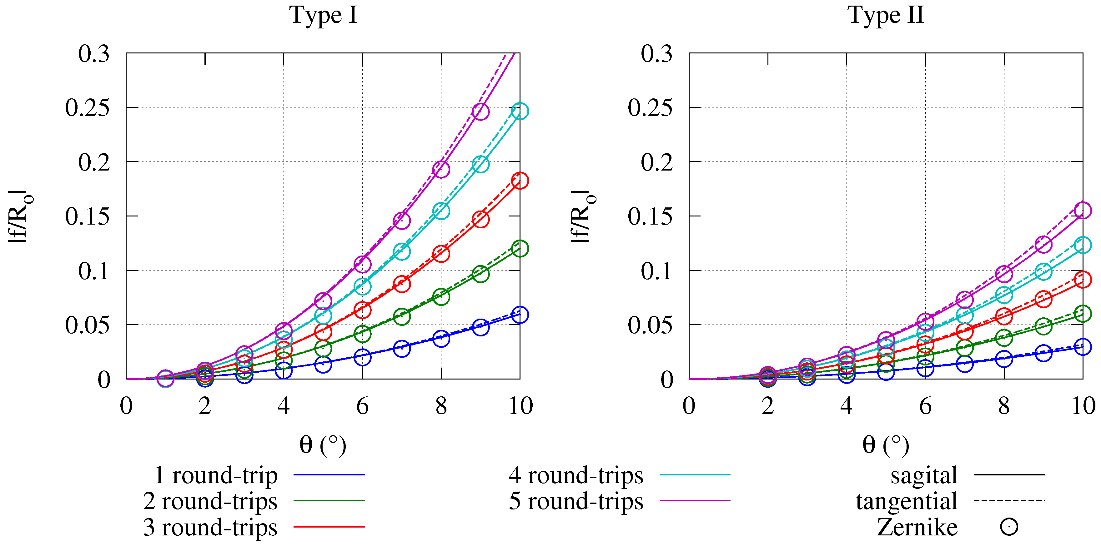
The absolute astigmatic deformation of the wavefront $|\raisebox{1ex}{$f$}\!\left/ \!\raisebox{-1ex}{$R$}\right.|$ in comparison for Type I and Type II is given in Figure 6. We used the absolute value here for a clearer presentation. The sagittal component results in a defocused beam, while the tangential direction results in a focused one. Again, we used the FRED software to benchmark the results from the matrix calculations. The only difference from the previous simulations is that the beam diameter is set to 3 mm and the wave length to 500 nm for Type I systems and 200 nm for Type II. Both changes were made to minimize the propagation effects in the system, which might disturb the comparability of both approaches and to assure a stable wavefront reconstruction. The actual wavefront radius was determined from the quadratic part of the sixth Zernike term. The results show a reasonably good agreement of both calculation methods.

The slight difference of the tangential and sagittal direction in the ABCD-matrix calculation further suggests that a slight spherical term is also added to the beam. As this is much smaller than the actual astigmatic terms, we refrained from further discussing it here.

Comparing Type I and Type II systems, we find that the astigmatic error for the same folding angle in a Type I system is twice the error in a Type II system. This can be explained logically, as the sources for the astigmatism in both systems are the large spherical mirrors, which are hit twice as often per round-trip in a Type I system. Furthermore, it can be seen that the astigmatic error for both systems increases over-proportionally with the folding angle and rather linearly with the number of round-trips. Hence, the folding angle in such a system should be chosen as small as reasonable possible.

5. Astigmatism due to Round-Trips

Another source of astigmatism within the presented relay imaging setups is introduced by the angular separation of the consecutive passes. This leads to a non-normal incidence on optics $L_1$ and $L_2$ in Type I systems and on $L_2$ in Type II systems. As before, we will use the basic system layouts for analyzing this effect.

The astigmatism will be included in the calculation by the same means as before, but using a varying incidence angle $\phi \left(k\right)$.

In the case of a Type II system, the sole source of astigmatism due to the round-trips is the mirror $L_2$. As the mirror $L_1$ is placed in the radius distance to the image plane, the incidence angle on $L_1$ is always normal to its surface. Including the astigmatism terms for $L_2$ according to Equations (20) and (21) for $G_3^m$ and $G_3^s$ for a single round-trip in the tangential and sagittal plane respectively results in:

$$\begin{array}{c}\hfill G_3^m=\left[\begin{array}{cc}1& 0\\ \frac{2cos\left(\phi \right(k\left)\right)-2}{fcos\left(\phi \right(k\left)\right)}& 1\end{array}\right]G_3^s=\left[\begin{array}{cc}1& 0\\ -\frac{2cos\left(\phi \right(k\left)\right)-2}{f}& 1\end{array}\right]\end{array}$$

(29)

Here, $\phi \left(k\right)$ is the incident angle, which varies for each round-trip. Given, that the system matrix represents an ideal lens in each plane, the inverse focal width $\raisebox{1ex}{$1$}\!\left/ \!\raisebox{-1ex}{$f$}\right.$ will just add up over the round trips. Hence, ${\left(\raisebox{1ex}{$1$}\!\left/ \!\raisebox{-1ex}{$R_o$}\right.\right)}_{m/s}$ after n round-trips can be expressed in each plane by a sum:

$$\begin{array}{c}\hfill {\left(\frac{1}{R_o}\right)}_m=-\frac{2}{f}·\sum _{k=1}^n\frac{cos\left(\phi \right(k\left)\right)-1}{cos\left(\phi \right(k\left)\right)}\end{array}$$

(30)

$$\begin{array}{c}\hfill {\left(\frac{1}{R_o}\right)}_s=\frac{2}{f}·\sum _{k=1}^{n}cos\left(\phi \left(k\right)\right)-1\end{array}$$

(31)

The maximum incidence angle ${\phi }_{max}$ can be calculated using:

$$\begin{array}{c}\hfill {\phi }_{max}=arctan\left(\frac{a_n}{2d_2}\right)=arctan\left(\frac{a_n}{4f}\right)\end{array}$$

(32)

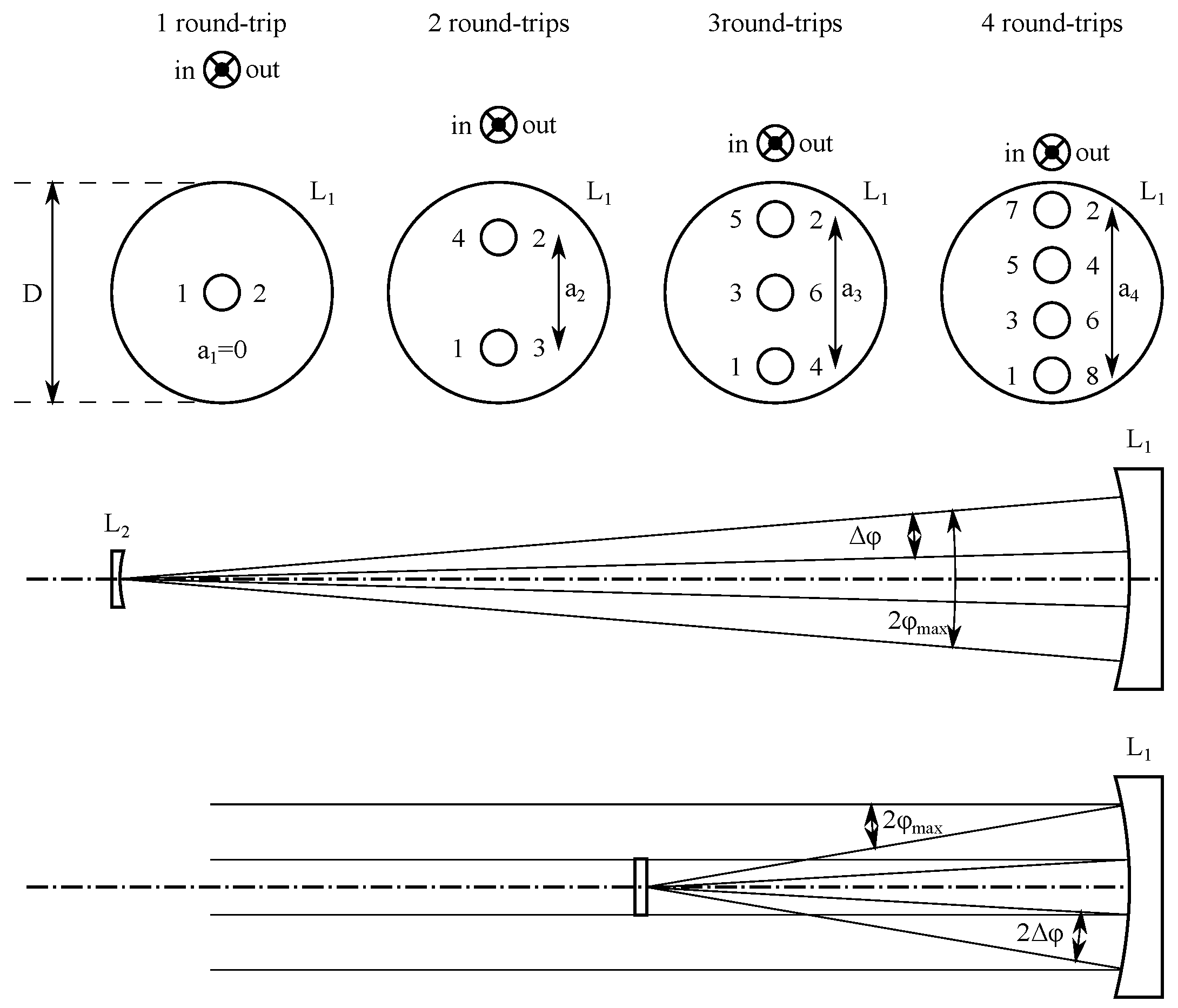
Here, $a_n$ is the maximum separation on the optic $L_1$, and it depends on the total number of round-trips n. $a_n$ again can be calculated assuming an optimum usage of the optics aperture D (cf. Figure 7) using:

$$\begin{array}{c}\hfill a_n=D·\frac{n-1}{n}\end{array}$$

(33)

Hence, the change in the incidence angle for each pass is given by:

$$\begin{array}{c}\hfill \Delta \phi =\frac{2{\phi }_{max}}{n-1}\end{array}$$

(34)

Now, $\phi \left(k\right)$ can be calculated by:

$$\begin{array}{c}\hfill \phi \left(k\right)={\phi }_{max}-(k-1)·\Delta \phi \end{array}$$

(35)

The wavefront radius $R_o$ of the sagittal and tangential plane of the astigmatic wavefront can be directly calculated using Equations (30) and (31).

For the case of Type I systems, such a closed solution no longer exists as both $L_1$ and $L_2$ generate the astigmatism during the round-trips and are not situated in an image plane or in an equivalent one. Hence, propagation effects will also be present. The handling of this type is nevertheless identical to the procedure described in the previous section for the astigmatism due to the folding angle except for a varying incidence angle $\phi \left(k\right)$ for every pass. The computations for $\phi \left(k\right)$ are the same as for Type II systems except for ${\phi }_{max}$, which is half of the value in Type I systems (cf. Figure 7):

$$\begin{array}{c}\hfill {\phi }_{max}=\frac{1}{2}·arctan\left(\frac{a_n}{2d_1}\right)=\frac{1}{2}·arctan\left(\frac{a_n}{2f}\right)\end{array}$$

(36)

For the following results, we used a collimated input beam according to the procedure in Section 4.

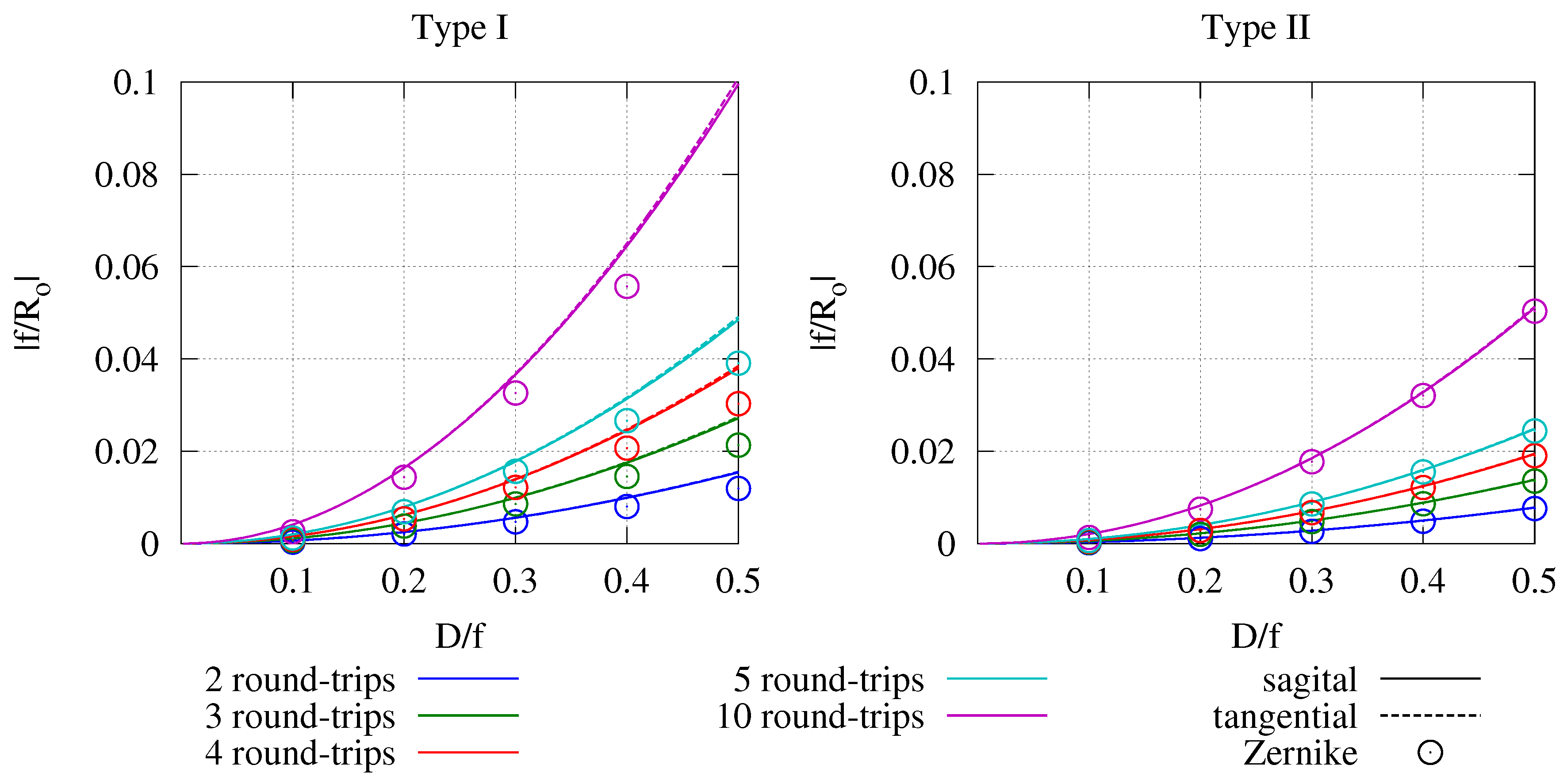
In Figure 8, the absolute astigmatic deformation of the wavefront as a function of the ratio between the diameter of the optic $L_1$ and its focal width is shown for both system types. Using $\raisebox{1ex}{$D$}\!\left/ \!\raisebox{-1ex}{$f$}\right.$ for the x-axis and $|\raisebox{1ex}{$f$}\!\left/ \!\raisebox{-1ex}{$R$}\right.|$ for the y-axis allows being independent from the exact focal width and the actual diameter of $L_1$. Hence, the results are applicable to a wide range of specific systems.

For the ray tracing simulation, systems identical to the ones used in Section 4 were used. To keep the influence of the folding angle negligible, this angle was fixed at 0.5°. Again, the ray-tracing results are in good agreement with the results from the simplified matrix model. Only for Type I systems, there seems to be a small deviation. This is most likely caused by a combination of a residual influence from the system’s folding angle and inaccuracies due to deviations in the propagation lengths, which are not included in the matrix model. These originate from the different distances between the image planes and $L_1$ and $L_2$ for different round-trips.

In Figure 9, the evolution of the astigmatic deformation over the round-trips is shown for sample systems with $\raisebox{1ex}{$D$}\!\left/ \!\raisebox{-1ex}{$f$}\right.$=0.3 with five and with 10 round-trips. It can be seen that due to the variation of φ over the individual passes, the main contribution to the wavefront deformation originates from the first and the last passes, while the intermediate passes add only a minor contribution. Furthermore, as there is virtually no change in the amount of deformation during the middle passes, the assumption that the chosen folding angle θ is sufficiently small to be negligible is confirmed.

In comparison to the astigmatism caused by the system’s folding angle, the obtained astigmatic deformation due to the round-trips is rather small. Nevertheless, for compact systems using a short focal length and a high number of round-trips, a considerable amount of deformation accumulates. In general, Type II systems are less critical by a factor of about two when using the focal length of the optic $L_1$ as a criterion.

6. Intrinsic Astigmatism Compensation Methods

Though astigmatism can be compensated in a straightforward way by using cylindrical optics for pre- and or post-compensation, it is often more convenient to have an intrinsic compensation. If this is achieved in each single pass of the system, it further reduces issues arising from the deformation of the beam profile on optics outside the image plane. The basic idea for such a compensation mechanism is to introduce astigmatism in two orthogonal directions with the same strength, which finally cancel each other. Such approaches were also discussed, e.g., in [3,10,11] for spectroscopic cells. We will present two approaches to achieve this within the presented Type I and Type II systems in the basic configurations, as described in Section 4.

In the case of the astigmatism within a Type I system caused by the folding angle of the arms, a compensating effect can be achieved when both arms are tilted in orthogonal planes by approximately the same amount (cf. Figure 10). Using this configuration in each plane, the beam will have one optic that is hit in the sagittal plane having a focal length of $f_s$ and one in the tangential plane having a focal length of $f_m$, where only the order is reversed for each beam axis. Hence, using Equation (4) results in:

$$\begin{array}{c}\hfill d_2=f_m+f_s=f·\left(cos\left(\theta \right)+\frac{1}{cos\left(\theta \right)}\right)\end{array}$$

(37)

Furthermore, Equation (3) must be fulfilled for both directions to achieve a complete compensation. An exchange of $f_1$ and $f_2$ in Equation (3) must not alter $d_1$ or $d_3$. This results in:

$$\begin{array}{c}\hfill d_1=d_3=\frac{f_m{f}_s^2+f_s{f}_m^2}{f_m^2+f_s^2}=f·cos\theta ·\frac{1+{cos}^2\theta }{1+{cos}^4\theta }\end{array}$$

(38)

A system with the according setup will be fully compensated, at least according to the matrix model. To cross-check this, we modeled a Type I system according to the ones presented in Section 4 with a folding angle of $\theta ={10}^{\circ }$ and five round-trips in the compensated arrangement. The resulting astigmatic deformation of the wavefront $\raisebox{1ex}{$f$}\!\left/ \!\raisebox{-1ex}{$R$}\right.$ was less then $4.5\times {10}^{-3}$ in all individual round-trips. Compared with the original value of $\raisebox{1ex}{$f$}\!\left/ \!\raisebox{-1ex}{$R$}\right.\approx 0.3$, this practically corresponds to a full compensation and proves the results from the matrix model. The residual deformation corresponds to the astigmatism caused by the round-trips, which is in the same range for the chosen configuration ($\raisebox{1ex}{$\mathrm{D}$}\!\left/ \!\raisebox{-1ex}{$\mathrm{f}$}\right.$ = 0.15; cf. Figure 8).

In the case of a Type II system, a compensation according to the just described method in Type I systems is only possible if the system is extended to get a second arm that can be tilted. In the following, we will discuss another way to compensate for astigmatism, which is based on compensating the astigmatism due to the folding angle with the astigmatism originating from the round-trips. We will use a basic Type II system (cf. Section 4) with 10 round-trips, a diameter of $L_1$ of 200 mm and a focal length of f = 500 mm, resulting in $\raisebox{1ex}{$D$}\!\left/ \!\raisebox{-1ex}{$f$}\right.$ = 0.3.

According to Section 5, the total astigmatic deformation due to the round-trips of the system $\raisebox{1ex}{$f$}\!\left/ \!\raisebox{-1ex}{$R_o$}\right.$ is calculated to be 0.0329 in the tangential plane and −0.0328 in the sagittal plane. Now, we use the matrix method according to Section 4 to numerically find an angle that will produce the inverse amount of astigmatic deformation. Therefore, the tangential and the sagittal plane will be exchanged in relation to the round-trip-based astigmatism to achieve a compensating effect. In the tangential plane, we find an angle of θ = 3.27° and in the sagittal plane an angle of θ = 3.29°. Hence, the compensation still has a small error. As a compromise, we use θ = 3.28°. Furthermore, there is a slight error due to the distances that would have to be adapted to the modified new focal lengths. We ignore this here, since the error is small.

The results for the astigmatic deformation from the ray-tracing of an accordingly designed Type II system are shown in Figure 11 in dependence of the round-trip number. As the generation of astigmatism due to the round-trips is strongest for the first and the last pass and nearly vanishes in between, the system is under-compensated for the first and the last passes, while it is over-compensated for the middle passes. The astigmatism due to θ is rather constant. In sum, this leads to an approximately perfect compensation after all passes, which demonstrates the validity of the compensation mechanism.

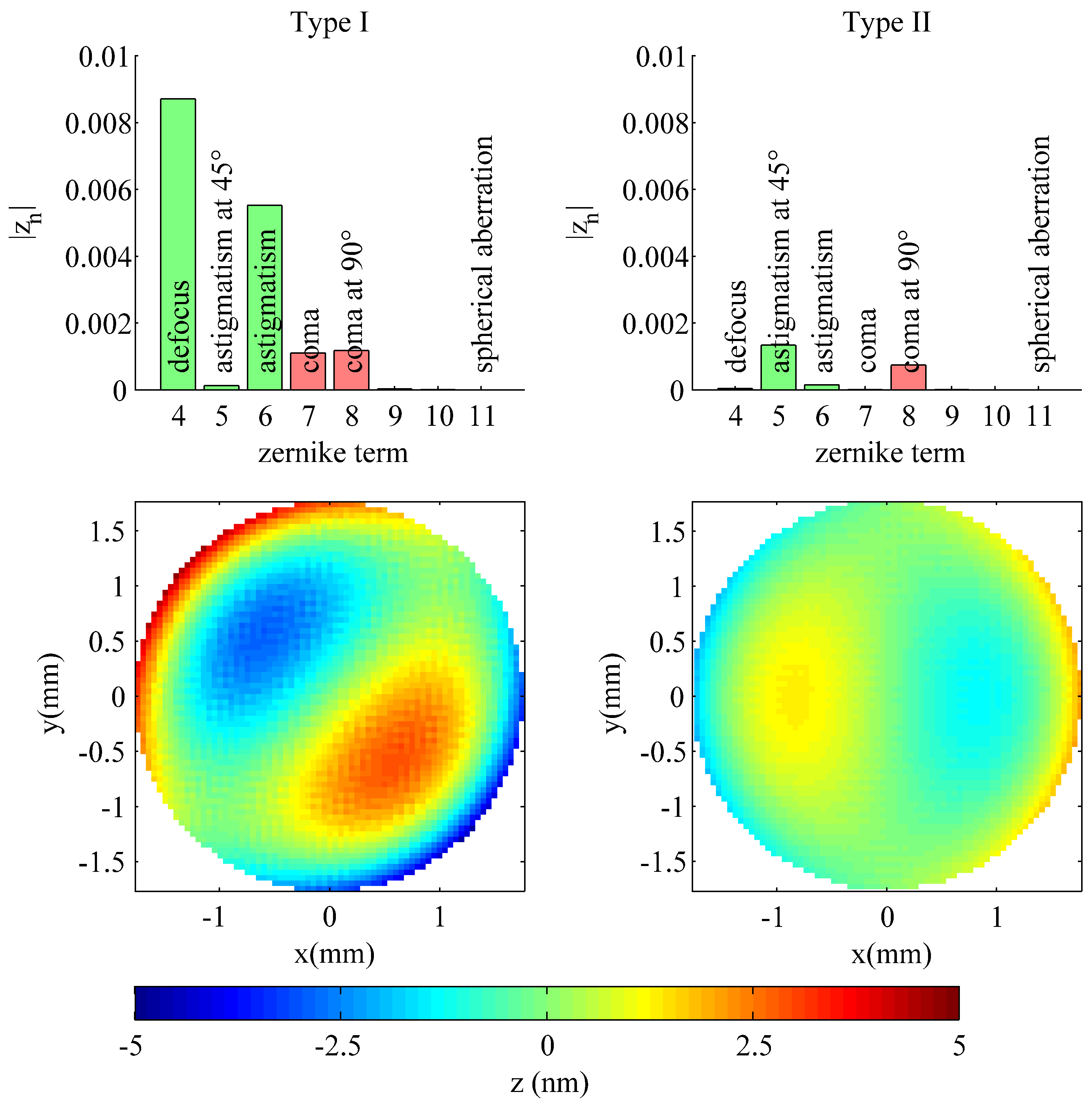
7. Higher Order Aberrations

For further discussion, we have also analyzed the higher order Zernike terms generated in the two astigmatism compensated systems described in Section 6. The derived terms are shown in Figure 12. It can be seen that the overall compensation of the astigmatism works slightly better in the Type II system as the round-trips were compensated, as well. Furthermore, there is some low amount of de-focus left in the Type I system, which can also be contributed to the round-trips. In the case of the Type II system, a very small amount of astigmatism under 45° still remains.

The higher order terms are even smaller than the residual terms for astigmatism in both compensated systems and should be of no practical relevance. The residual distortions are dominated by coma, which has basically the same origin as the astigmatism. Higher order Zernike terms are negligible. The total wavefront error contributed by all terms higher than six is below 10 nm for the Type I system and 2 nm for the Type II system. The corresponding wave forms are shown in the lower part of Figure 12 after subtracting all terms lower than seven. Here, also the coma can be clearly identified.

8. Conclusions

In this work, we presented a matrix model for the categorization and evaluation of imaging setups for multi-pass laser amplifiers in which the imaging elements are repeatedly used to reduce the total number of optics needed. It was found that such systems can be classified into two basic types, which we referred to as Type I and Type II. Here, Type I systems resemble a double-passed telescope, with a total of four interactions with imaging elements. Type II systems resemble a three-element imaging with three interactions of imaging elements per round-trip, accordingly. With the matrix formalism, we directly derived laws for the distances between the optics in dependence of their individual focal lengths.

Further we discussed the influence of aberrations in the setup of such systems. It was shown that both types of systems can be used to internally compensate a thermal lens within their image plane. Correction terms for the distances were again derived by the matrix formalism accordingly.

The problem of astigmatism was analyzed and quantified as well in dependence of the inevitable folding angle of the arms in mirror-based systems as for the tilted incidence required to geometrically separate individual round-trips for in- and out-put coupling. It was found that comparing both system types, equally dimensioned Type II systems exhibit a lower astigmatism by a factor of about two.

Further using the matrix formalism, we demonstrated different methods, where due to geometrical folding, an intrinsic compensation of the system’s astigmatism could be achieved. Here, a Type I system was compensated for the folding angle of the arms, while in a Type II system, compensation of the arms’ folding angle was achieved with the astigmatism generated by the round-trips. In both cases, a nearly complete compensation was demonstrated.

All presented calculations with the matrix method were cross-checked by analyzing the Zernike polynomials of wavefronts calculated by coherent ray-tracing of representative systems in the commercial software FRED. Hereby, a very good agreement between both calculation methods was achieved, proving the validity of the matrix method. The ray-tracing software also allowed analyzing higher order Zernike terms. It was found that both systems exhibit practically negligible higher order distortions even for a high number of round-trips and comparably short focal length.

From a practical point of view, the results of our calculations suggest that, in general, Type II systems show a superior performance when compared to Type I systems. This statement is supported by the lower amount of astigmatic aberrations generated under similar conditions, the higher degree of compensation of effects from a thermal lens and by the overall lower amount of residual aberrations in a compensated system. The latter point is even more pronounced, as the investigated Type II system allows twice the number of passes, and therefore, it is also more compact. Furthermore, from an engineer’s point of view, Type II systems seems to be more convenient as the total number of optics is smaller, in particular for the large diameter optics, on which the round trips are separated. Until now, mostly Type I systems can be found in the literature, but we believe that the use of Type II systems can lead to more compact laser designs with less aberrations, where shorter focal lengths can be employed.