Dynamical Systems Properties of a Mathematical Model for the Treatment of CML

Abstract

A mathematical model for the treatment of chronic myeloid leukemia (CML) through a combination of tyrosine kinase inhibitors and immunomodulatory therapies is analyzed as a dynamical system for the case of constant drug concentrations. Equilibria and their stability are determined and it is shown that, depending on the parameter values, the model exhibits a variety of behaviors which resemble the chronic, accelerated and blast phases typical of the disease. This work provides qualitative insights into the system which should be useful for understanding the interaction between CML and the therapies considered here.

1. Introduction

Chronic myeloid leukemia (CML) is a hematologic cancer that accounts for about 15% of all leukemias in adults and is characterized by uncontrolled expansion of myeloid cells in the bone marrow and their accumulation in the blood [1]. The progression of the disease can be divided into three phases denoted chronic, accelerated and blast [1]. The chronic phase can last several years with levels of immature white blood cells (blasts) growing steadily but at a low rate. Once the disease enters the accelerated or blast phase, cells proliferate rapidly and the disease can be lethal within a few months if not treated. Current standard of care includes targeted tyrosine kinase inhibitors (TKIs), which have significantly improved long-term survival rates [2].

Responses to certain treatments have offered evidence of an immune component in the disease [3]. Early indications were provided by a correlation between incidence of graft-vs-host disease and improved leukemia-free survival in CML patients who had received allogeneic stem cell transplants [4]. Additionally, treatment with interferons (which are known to be immunomodulatory) has led to complete or partial responses in some fraction of CML patients [5]. More recently, studies that include immunomodulatory therapies such as nivolumab have been initiated [6].

Mathematical modeling of CML dynamics has a history dating back to the late 1960s with early work of Rubinow and Lebowitz [7,8]. Models by Fokas et al. [9] in the 1990s focused on maturation and proliferation of T-cell precursors. In 2004, Moore and Li [10] published a model of CML dynamics, which accounts for the actions of naive and effector T-cells separately. In [11], this model was analyzed as an optimal control problem. The model presented here first appeared in [12] and models the immune system effects with one compartment, and separates the CML cells into quiescent and proliferating classes. The rationale behind this new model is the ability to represent certain types of therapies for use in combination treatment. These therapies are: a BCR-ABL1 tyrosine kinase inhibitor (e.g., a therapy such as imatinib), an immunomodulatory therapy (e.g., a therapy such as nivolumab), and a therapy that combines both actions (e.g., a therapy such as dasatinib).

The model introduced in [12] is reviewed in Section 2 and then analyzed as a dynamical system with constant drug concentrations in Section 3. The analysis is carried out theoretically for values of parameters covering a range of dynamic possibilities. As will be seen, there are parameter values for which the model can have an asymptotically stable equilibrium point in which all the state variables are positive. This could be interpreted as disease control through continuous therapy. As parameters change, the system can become unstable and undergo exponential growth, representing the accelerated or blast phases of the disease. Our analysis incorporates constant drug concentrations, and thus provide insights into the dynamics both without and with treatment. In particular, we analyze how an increase in the levels of each of the three treatments affects the values of all three populations, the two types of leukemia cells and the strength of the immune effect. The combination of theoretical analysis and simulations is intended to shed some light on understanding the long-term dynamics of this disease under treatment.

2. A Mathematical Model for the Treatment of CML with BCR-ABL1-Targeted and Immunomodulatory Drugs

The mathematical model below was originally published in [12] in 2015.

2.1. A Brief Review of the Mathematical Model

Let Q be the concentration of quiescent leukemic cells, P the concentration of proliferating leukemic cells, and E the strength of immune system effects. We will consider E to represent effector T cell concentration levels, and will refer to E in the remainder as a concentration of effector T cells. The model contains three controls $u_1$, $u_2$ and $u_3$ that all denote normalized levels of different therapies. The roles of the specific drugs are illustrated in Figure 1 taken from [12] with arrows indicating amplification of effects and vertical bars indicating inhibition. The control $u_1$ represents the normalized concentration of a BCR-ABL1 inhibitor (such as imatinib) that mainly has an inhibitory effect on the highly-proliferating leukemic cells; $u_2$ is a BCR-ABL1 inhibitor that inhibits BCR-ABL1 that also has immune effects (such as dasatinib); while $u_3$ represents an immunomodulatory compound (such as nivolumab).

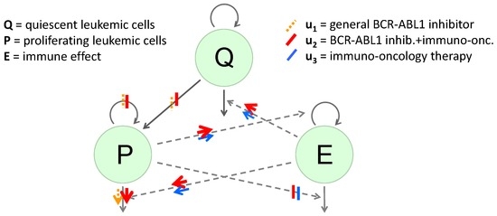
Figure 1. Diagram of the dynamical system. The green circular areas represent the “populations" included in the model. Solid arrows extending from or to the populations represent changes in numbers, with inward-pointing arrows representing increases and outward-pointing arrows decreases. Dashed arrows indicate indirect effects on those increases or decreases. Bars represent inhibition of a production or an indirect effect, due to the represented treatment; arrows represent amplification of a rate or an indirect effect. The effects of the general BCR-ABL1 inhibitor $u_1$ are shown using orange dashed bars and arrows, the effects of the BCR-ABL1 inhibitor $u_2$ which also has immune effects are shown using wide red solid bars and arrows and the effects of the immunomodulatory compound $u_3$ are shown using blue solid bars and arrows.

Representing the pharmacodynamic effects of the drugs using Michaelis-Menten terms results in the following equations:

$$\begin{array}{cc}\hfill \frac{dQ}{dt}& =r_{Q}Q-{\delta }_Q\left[1+\left(1+\frac{U{2}_{max,1}{u}_2}{U2C_{50}+u_2}\right)\left(1+\frac{U{3}_{max,1}{u}_3}{U3C_{50}+u_3}\right)\frac{E_{max,1}E}{E{C}_{50}+E}\right]Q,\hfill \end{array}$$

(1)

$$\begin{array}{cc}\hfill \frac{dP}{dt}=& \left(1-\frac{U{1}_{max,1}{u}_1}{U1C_{50}+u_1}\right)\left(1-\frac{U{2}_{max,2}{u}_2}{U2C_{50}+u_2}\right)\left[k_{P}Q+r_{P}Pln\left(\frac{P_{\mathrm{ss}}}{P}\right)\right]\hfill \\ & -{\delta }_P\left(1+\frac{U{1}_{max,2}{u}_1}{U1C_{50}+u_1}\right)\left(1+\frac{U{2}_{max,3}{u}_2}{U2C_{50}+u_2}\right)P\hfill \\ & -{\delta }_P\left(1+\frac{U{2}_{max,1}{u}_2}{U2C_{50}+u_2}\right)\left(1+\frac{U{3}_{max,1}{u}_3}{U3C_{50}+u_3}\right)\frac{E_{max,2}E}{E{C}_{50}+E}P,\hfill \end{array}$$

(2)

$$\begin{array}{cc}\hfill \frac{dE}{dt}=& s_E\left[1+\left(1+\frac{U{2}_{max,4}{u}_2}{U2C_{50}+u_2}\right)\left(1+\frac{U{3}_{max,2}{u}_3}{U3C_{50}+u_3}\right)\frac{P_{max,1}P}{P{C}_{50}+P}\right]Eln\left(\frac{E_{\mathrm{ss}}}{E}\right)\hfill \\ & -{\delta }_E\left[1+\left(1-\frac{U{2}_{max,5}{u}_2}{U2C_{50}+u_2}\right)\left(1-\frac{U{3}_{max,3}{u}_3}{U3C_{50}+u_3}\right)\frac{P_{max,2}P}{P{C}_{50}+P}\right]E.\hfill \end{array}$$

(3)

In this system, all parameters are non-negative. For $P=0$ or $E=0$, we extend the system by defining it using the limits as $P\to 0$ or $E\to 0$, respectively. The cell count numbers for Q are relatively small and are therefore modeled by an exponential function with growth coefficient $r_Q$. For the proliferating cells P we model growth with a Gompertz function, as Afenya and Calderón state that this is best for describing CML growth [13]. The immune effect E (effector T cells) also has its rate of increase modeled by a Gompertz function, so as to have approximately exponential growth when numbers are very small, but still be bounded above. In the populations P and E, replication rate constants are represented by $r_P$ and $s_E$, and carrying capacities (or steady states) by $P_{\mathrm{ss}}$ and $E_{\mathrm{ss}}$, respectively. The natural death rate constants of the respective populations are denoted by ${\delta }_Q$, ${\delta }_P$ and ${\delta }_E$. The population Q consists of leukemic cells that are quiescent. Some or all of quiescent leukemic cells may be stem cells [14]. When quiescent cells divide, one copy is assumed to be the same kind as the original cell while the second copy may differentiate further into a proliferating type. For this reason, the transition term $k_{P}Q$ is not subtracted from the quiescent cell population in (1). This term represents the rate at which quiescent cells produce differentiated proliferating cancer cells, with the population Q the source for the population P.

The control variables represent the concentrations of the respective drugs, and their effects (pharmacodynamics) are modeled by Michaelis-Menten terms with different maximum effectiveness on the various populations. In modeling the combined drug actions it is assumed that any two drugs act independently of each other. Thus the term

$$\left(1-\frac{U{1}_{max,1}{u}_1}{U1C_{50}+u_1}\right)\left(1-\frac{U{2}_{max,2}{u}_2}{U2C_{50}+u_2}\right)\left[k_{P}Q+r_{P}Pln\left(\frac{P_{\mathrm{ss}}}{P}\right)\right]$$

represents the effects that drugs 1 and 2 have on decreasing the proliferation of the population P. A term of the type

$$-{\delta }_Q\left(1+\frac{U{2}_{max,1}{u}_2}{U2C_{50}+u_2}\right)\left(1+\frac{U{3}_{max,1}{u}_3}{U3C_{50}+u_3}\right)\frac{E_{max,1}E}{E{C}_{50}+E}Q$$

represents the enhancement of the actions of the effector T cells E on the quiescent cells Q as a consequence of the activities of drugs 2 and 3. In each of the equations, the enhancement and inhibition effects of the drugs by means of the immune system are modeled additively.

The “$C_{50}$” parameters $U1C_{50}$, $U2C_{50}$, and $U3C_{50}$ represent the concentrations required to achieve half of the maximal effects of $u_1$, $u_2$, and $u_3$, respectively. These and $E{C}_{50}$ and $P{C}_{50}$ are assumed to be fixed across effects being modeled. These represent “potency” levels depending intrinsically on the particular therapy or population, and not on the setting of the effect. The maximum possible effect size is allowed to depend on the setting.

The equations above represent a semi-mechanistic, fit-for-purpose, minimal model. It is minimal in the sense that it only includes the levels of cell interactions needed to allow the controls to have their expected effects. Some of the terms are based on models validated with data, but other terms take forms that are more heuristic. For example, all of the control effect terms take a Michaelis-Menten or “Emax” form. This is because we wish to model very small effect at low levels of drug, as well as a limiting or asymptotic maximal effect at high levels of drugs. We chose the simplest among the models with this behavior that are typically used in drug development [15].

The states, controls, and related parameters are listed in Table 1 and Table 2. Table 1 gives those parameters that are unrelated to the drug actions and make up the untreated, or uncontrolled, system; Table 2 lists the treatment-specific parameters in the model. In this paper, we do not fit or fix specific parameter values, and instead analyze the dynamic properties of the system (1)–(3) for large ranges of possible values. We include in the tables below two different sets of numerical values that we use to illustrate the dynamic properties of the system. These parameter values are purely for numerical illustration and do not reflect specific model fits or therapies. The focus of this paper is the mathematical analysis of the entire system rather than an analysis for particular parameter values.

Table 1. States and parameters for the dynamical system.

Symbol	Interpretation	Units	Values Used in Figure 2	Values Used in Figure 3 and Figure 4
Q	concentration of quiescent leukemic cells	${10}^2$ cells/mL
P	concentration of proliferating leukemic cells	${10}^7$ cells/mL
$P_{\mathrm{ss}}$	carrying capacity of proliferating	${10}^7$ cells/mL	10	15
	leukemic cells
E	effector T cells	$2\times {10}^3$ cells/mL
$E_{\mathrm{ss}}$	carrying capacity of effector T cells	$2\times {10}^3$ cells/mL	$1.75$	$2.25$
$r_Q$	replication rate constant of quiescent cells	1/day		$0.02$
${\delta }_Q$	natural death rate constant of quiescent cells	1/day		$0.005$
$k_P$	rate constant for quiescent cells Q	1/day		$0.10$
	differentiating into proliferating cells P
$r_P$	replication rate constant of proliferating	1/day	8	$0.30$
	leukemic cells
${\delta }_P$	natural death rate constant of proliferating	1/day	$0.75$	$0.02$
	leukemic cells
$s_E$	growth rate constant for effector T cells	1/day	$0.25$	$0.01$
${\delta }_E$	natural death rate constant of effector T cells	1/day	$0.25$	$0.005$
$P_{max,1}$	maximum stimulation effect of proliferating		2	$0.50$
	leukemic cells P on effector T cells E
$P_{max,2}$	maximum inhibition effect of proliferating		5	$0.20$
	leukemic cells P on effector T cells E
$P{C}_{50}$	size of P with half the maximum effect	1/mL	${10}^7$	${10}^7$
$E_{max,1}$	maximum effect of effector T cells E on			5
	quiescent leukemic cells Q
$E_{max,2}$	maximum effect of effector T cells E on		1	5
	proliferating leukemic cells P
$E{C}_{50}$	size of E with half the maximum effect	1/mL	2000	2000

Table 2. Controls and pharmacodynamic parameters.

Symbol	Interpretation	Values Used in Figure 2	Values Used in Figure 3 and Figure 4
$u_1$	normalized concentration of a general BCR-ABL1
	inhibitor (e.g., imatinib)
$U{1}_{max,1}$	maximum possible effect of $u_1$ on slowing	$0.8$	$0.8$
	transfer of quiescent cells Q into P and
	inhibiting growth of proliferating cells P
$U{1}_{max,2}$	maximum possible effect of $u_1$ on death of	10	2
	proliferating cells P
$U1C_{50}$	concentration of $u_1$ that gives half the maximum effect	1	1
$u_2$	normalized concentration of a BCR-ABL1 inhibitor
	which also has immunomodulatory effects
	(e.g., dasatinib)
$U{2}_{max,1}$	maximum possible effect of $u_2$ on death of leukemic	2	$0.01$
	cells (the same for P and Q)
$U{2}_{max,2}$	maximum possible effect of $u_2$ slowing new P from	$0.6$	$0.03$
	Q and inhibiting growth of proliferating cells P
$U{2}_{max,3}$	maximum possible effect of $u_2$ on	10	$0.01$
	death of proliferating cells P
$U{2}_{max,4}$	maximum possible effect of $u_2$ on	10	$0.025$
	stimulating proliferation of effector T cells
$U{2}_{max,5}$	maximum possible effect of $u_2$ on	$0.4$	$0.02$
	prevention of the death of effector T cells
$U2C_{50}$	concentration of $u_2$ that gives half the maximum effect	$0.6$	$0.8$
$u_3$	normalized concentration of an immunomodulatory
	d agent (e.g., nivolumab)
$U{3}_{max,1}$	maximum possible effect of $u_3$ on death of leukemic	5	$0.02$
	cells (the same for P and Q)
$U{3}_{max,2}$	maximum possible effect of $u_3$ on	5	$0.05$
	stimulating proliferation of effector T cells
$U{3}_{max,3}$	maximum possible effect of $u_3$ on	$0.7$	$0.07$
	prevention of the death of effector T cells
$U3C_{50}$	concentration of $u_3$ that gives half the maximum effect	$0.7$	$0.7$

2.2. Scaling of Parameters

We note that the dynamical system has various groups of symmetries that can be used to scale the variables and controls. Here we normalize all the “$C_{50}$” parameter values to 1 by rescaling the corresponding variables in terms of these quantities. This simply minimizes the number of parameters to be considered in the analysis of the system. For example, let $Q_{\mathrm{ref}}$ be a constant to be determined later, and define

$$\tilde{Q}=\frac{Q}{Q_{\mathrm{ref}}},\tilde{P}=\frac{P}{P{C}_{50}},\tilde{E}=\frac{E}{E{C}_{50}},$$

and

$${\tilde{u}}_1=\frac{u_1}{U1C_{50}},{\tilde{u}}_2=\frac{u_2}{U2C_{50}},{\tilde{u}}_3=\frac{u_3}{U3C_{50}}.$$

Then we have that

$$\frac{E}{E{C}_{50}+E}=\frac{\tilde{E}}{1+\tilde{E}}$$

and analogously for the other terms.

For the differential equations, we obtain

$$\begin{array}{cc}\hfill \frac{d\tilde{Q}}{dt}& =\frac{1}{Q_{\mathrm{ref}}}\frac{dQ}{dt}\hfill \\ & =\frac{1}{Q_{\mathrm{ref}}}\left\{r_{Q}Q-{\delta }_Q\left[1+\left(1+\frac{U{2}_{max,1}{\tilde{u}}_2}{1+{\tilde{u}}_2}\right)\left(1+\frac{U{3}_{max,1}{\tilde{u}}_3}{1+{\tilde{u}}_3}\right)\frac{E_{max,1}\tilde{E}}{1+\tilde{E}}\right]Q\right\}\hfill \\ & =r_Q\tilde{Q}-{\delta }_Q\left[1+\left(1+\frac{U{2}_{max,1}{\tilde{u}}_2}{1+{\tilde{u}}_2}\right)\left(1+\frac{U{3}_{max,1}{\tilde{u}}_3}{1+{\tilde{u}}_3}\right)\frac{E_{max,1}\tilde{E}}{1+\tilde{E}}\right]\tilde{Q}.\hfill \end{array}$$

Under this scaling all remaining parameters in this equation are invariant and need not be changed. Similarly,

$$\begin{array}{ccc}\hfill \frac{d\tilde{P}}{dt}& =& \frac{1}{P{C}_{50}}\frac{dP}{dt}\hfill \\ & =& \frac{1}{P{C}_{50}}\left\{\left(1-\frac{U{1}_{max,1}{\tilde{u}}_1}{1+{\tilde{u}}_1}\right)\left(1-\frac{U{2}_{max,2}{\tilde{u}}_2}{1+{\tilde{u}}_2}\right)\left[k_{P}Q+r_{P}Pln\left(\frac{P_{\mathrm{ss}}}{P}\right)\right]\right.\hfill \\ & & -{\delta }_P\left(1+\frac{U{1}_{max,2}{\tilde{u}}_1}{1+{\tilde{u}}_1}\right)\left(1+\frac{U{2}_{max,3}{\tilde{u}}_2}{1+{\tilde{u}}_2}\right)P\hfill \\ & & \left.-{\delta }_P\left(1+\frac{U{2}_{max,1}{\tilde{u}}_2}{1+{\tilde{u}}_2}\right)\left(1+\frac{U{3}_{max,1}{\tilde{u}}_3}{1+{\tilde{u}}_3}\right)\frac{E_{max,2}\tilde{E}}{1+\tilde{E}}P\right\}\hfill \\ & =& \left(1-\frac{U{1}_{max,1}{\tilde{u}}_1}{1+{\tilde{u}}_1}\right)\left(1-\frac{U{2}_{max,2}{\tilde{u}}_2}{1+{\tilde{u}}_2}\right)\left[\left(k_P\frac{Q_{\mathrm{ref}}}{P{C}_{50}}\right)\tilde{Q}+r_P\tilde{P}ln\left(\frac{P_{\mathrm{ss}}}{\tilde{P}·P{C}_{50}}\right)\right]\hfill \\ & & -{\delta }_P\left(1+\frac{U{1}_{max,2}{\tilde{u}}_1}{1+{\tilde{u}}_1}\right)\left(1+\frac{U{2}_{max,3}{\tilde{u}}_2}{1+{\tilde{u}}_2}\right)\tilde{P}\hfill \\ & & -{\delta }_P\left(1+\frac{U{2}_{max,1}{\tilde{u}}_2}{1+{\tilde{u}}_2}\right)\left(1+\frac{U{3}_{max,1}{\tilde{u}}_3}{1+{\tilde{u}}_3}\right)\frac{E_{max,2}\tilde{E}}{1+\tilde{E}}\tilde{P},\hfill \end{array}$$

and

$$\begin{array}{ccc}\hfill \frac{d\tilde{E}}{dt}& =& \frac{1}{E{C}_{50}}\frac{dE}{dt}\hfill \\ & =& s_E\left[1+\left(1+\frac{U{2}_{max,4}{\tilde{u}}_2}{1+{\tilde{u}}_2}\right)\left(1+\frac{U{3}_{max,2}{\tilde{u}}_3}{1+{\tilde{u}}_3}\right)\frac{P_{max,1}\tilde{P}}{1+\tilde{P}}\right]\tilde{E}ln\left(\frac{E_{\mathrm{ss}}}{\tilde{E}·E{C}_{50}}\right)\hfill \\ & & -{\delta }_E\left[1+\left(1-\frac{U{2}_{max,5}{\tilde{u}}_2}{1+{\tilde{u}}_2}\right)\left(1-\frac{U{3}_{max,3}{\tilde{u}}_3}{1+{\tilde{u}}_3}\right)\frac{P_{max,2}\tilde{P}}{1+\tilde{P}}\right]\tilde{E}.\hfill \end{array}$$

Thus, if we re-scale $k_P$ as

$${\tilde{k}}_P=\frac{Q_{\mathrm{ref}}}{P{C}_{50}}{k}_P$$

(4)

and the steady-state values as

$${\tilde{P}}_{\mathrm{ss}}=\frac{P_{\mathrm{ss}}}{P{C}_{50}}\mathrm{and}{\tilde{E}}_{\mathrm{ss}}=\frac{E_{\mathrm{ss}}}{E{C}_{50}},$$

(5)

then formally the equations are the same as before with all “$C_{50}$” values in the Michaelis-Menten expressions normalized to 1. All other parameters remain unchanged and even their interpretation is the same as before. For the theoretical analysis and numerical computations this eliminates five parameters and introduces a favorable scaling to the variables. Naturally, the original parameters are still calculated for an interpretation of the results.

3. System Properties for Constant Concentrations

CML has three distinct phases, a chronic one that can last from three to five years, during which leukemic cell counts are low but may grow steadily, and accelerated and blast phases that may last for a only a few months and are characterized by higher cell counts or a rapid increase in cell counts followed by death of the patient [10]. Here we analyze the dynamical system to determine if it can capture such features.

3.1. Reduction to the Uncontrolled System and Basic Dynamical System Properties

We carry out the dynamical systems analysis for constant controls, i.e., concentrations. We do not explicitly include pharmacokinetics (fluctuations in concentrations that depend on doses). The treatments considered are either administered daily or have long half-lives, and such pharmacokinetics are not expected to be significant for the treatment periods we consider here (five years or longer). We also mention the 2009 paper by Shudo et al. [16] that supports this assumption in the setting of hepatitis C.

Keeping the “$C_{50}$” parameters in their original formulation in the controls, we define new drug-dependent parameters as

$$\begin{array}{cc}\hfill {\widehat{k}}_P& =\left(1-\frac{U{1}_{max,1}{u}_1}{U1C_{50}+u_1}\right)\left(1-\frac{U{2}_{max,2}{u}_2}{U2C_{50}+u_2}\right)k_P,\hfill \\ \hfill {\widehat{r}}_P& =\left(1-\frac{U{1}_{max,1}{u}_1}{U1C_{50}+u_1}\right)\left(1-\frac{U{2}_{max,2}{u}_2}{U2C_{50}+u_2}\right)r_P,\hfill \\ \hfill {\widehat{\delta }}_P& =\left(1+\frac{U{1}_{max,2}{u}_1}{U1C_{50}+u_1}\right)\left(1+\frac{U{2}_{max,3}{u}_2}{U2C_{50}+u_2}\right){\delta }_P,\hfill \\ \hfill {\widehat{E}}_{max,1}& =\left(1+\frac{U{2}_{max,1}{u}_2}{U2C_{50}+u_2}\right)\left(1+\frac{U{3}_{max,1}{u}_3}{U3C_{50}+u_3}\right)E_{max,1},\hfill \\ \hfill {\widehat{E}}_{max,2}& =\frac{\left(1+\frac{U{2}_{max,1}{u}_2}{U2C_{50}+u_2}\right)\left(1+\frac{U{3}_{max,1}{u}_3}{U3C_{50}+u_3}\right)}{\left(1+\frac{U{1}_{max,2}{u}_1}{U1C_{50}+u_1}\right)\left(1+\frac{U{2}_{max,3}{u}_2}{U2C_{50}+u_2}\right)}{E}_{max,2},\hfill \\ \hfill {\widehat{P}}_{max,1}& =\left(1+\frac{U{2}_{max,4}{u}_2}{U2C_{50}+u_2}\right)\left(1+\frac{U{3}_{max,2}{u}_3}{U3C_{50}+u_3}\right)P_{max,1},\hfill \\ \hfill {\widehat{P}}_{max,2}& =\left(1-\frac{U{2}_{max,5}{u}_2}{U2C_{50}+u_2}\right)\left(1-\frac{U{3}_{max,3}{u}_3}{U3C_{50}+u_3}\right)P_{max,2}.\hfill \end{array}$$

With these identifications, the dynamical system with constant controls is identical with the uncontrolled system and therefore, without loss of generality, the analysis can be done on the uncontrolled system. Returning to the original notation without the carets, we thus consider the following equations:

$$\begin{array}{cc}\hfill \frac{dQ}{dt}& =\left[r_Q-{\delta }_Q\left(1+\frac{E_{max,1}E}{1+E}\right)\right]Q,\hfill \end{array}$$

(6)

$$\begin{array}{cc}\hfill \frac{dP}{dt}& =k_{P}Q+\left[r_{P}ln\left(\frac{P_{\mathrm{ss}}}{P}\right)-{\delta }_P\left(1+\frac{E_{max,2}E}{1+E}\right)\right]P,\hfill \end{array}$$

(7)

$$\begin{array}{cc}\hfill \frac{dE}{dt}& =\left[s_E\left(1+\frac{P_{max,1}P}{1+P}\right)ln\left(\frac{E_{\mathrm{ss}}}{E}\right)-{\delta }_E\left(1+\frac{P_{max,2}P}{1+P}\right)\right]E.\hfill \end{array}$$

(8)

The model with an exponential growth term on Q has various long-term behaviors. These include the extremes in which Q decays exponentially to zero or grows exponentially beyond limits, but there also is the possibility that nontrivial equilibrium points $(Q_{*},P_{*},E_{*})$ exist for which all three populations are positive. The first case corresponds to a scenario in which the patient goes into a stable deep molecular response. For the uncontrolled system, this may not seem to be of interest, but since the model includes the case with controls, this gives us information about which combinations of constant concentrations of the drugs would lead to an eradication of Q. The case of exponential growth may characterize the accelerated or blast phase as these phases have short doubling times [17]. The conditions under which this is the long-term behavior of the system give information about what controls are needed for successful treatment. An asymptotically stable equilibrium point $(Q_{*},P_{*},E_{*})$ with positive values could be interpreted as describing a subset of the chronic phase where net growth rate is zero, controlled by therapy or immune effects. Depending on the values of the parameters, this equilibrium point may be stable or unstable. Since in real life parameters may not be constant, bifurcation phenomena would be a mathematical description of the transition from chronic to the accelerated or blast phases. Knowing the parameter values when this may occur would be of interest. Our aim in the following is thus to determine the asymptotic behavior of the trajectories of the system.

We start with some basic properties. The positive orthant

$$\mathbb{P}=\left\{(Q,P,E):Q>0,P>0,E>0\right\}$$

is positively invariant for the dynamics. This is because the planes $Q=0$ and $E=0$ are invariant under Equations (6) and (8) and $\dot{P}\ge k_{P}Q$ whenever $P=0$. Thus, starting at a positive initial condition $(Q_0,P_0,E_0)$, it follows that the solutions remain positive for all times. For the long-term behavior of the system, the equilibrium solutions in the closure of $\mathbb{P}$, $\overline{\mathbb{P}}=\mathrm{clos}\left(\mathbb{P}\right)$, also matter. Recall that the system is defined and continuous on $\overline{\mathbb{P}}$ due to the use of the limits as $P\to 0$ and $E\to 0$ in place of $P=0$ and $E=0$, respectively. The vector field defining the P and E dynamics is not continuously differentiable at $P=0$ or $E=0$, but these values are repelling and thus this does not become an issue.

Lemma 1.

The equilibrium solution $E_{*}=0$ is repelling: there exists a positive threshold $E_{\Delta }<E_{\mathrm{ss}}$ such that $\frac{dE}{dt}$ is positive on $(0,E_{\Delta }]$. In particular, once $E_{\mathrm{ss}}>E\left(\tau \right)\ge E_{\Delta }$, then $E\left(t\right)\ge E_{\Delta }$ for all $t\ge \tau$. Furthermore, for $E\left(0\right)<E_{\mathrm{ss}}$, E will remain below $E_{\mathrm{ss}}$.

Proof. 

The terms in the last parentheses in Equation (8) are bounded between 1 and $1+P_{max,2}$ and thus, as $E\to 0$, the Gompertzian growth dominates the dynamics. Specifically, let

$$E_{\Delta }=E_{\mathrm{ss}}exp\left(-\frac{{\delta }_E}{s_E}\left(1+P_{max,2}\right)\right);$$

then $E_{\Delta }\le E_{\mathrm{ss}}$ and for $E<E_{\Delta }$ we have that $\frac{dE}{dt}>0$. Furthermore, for $E=E_{\mathrm{ss}}$, Equation (8) reduces to $\frac{dE}{dt}=-{\delta }_E\left(1+\frac{P_{max,2}P}{1+P}\right)E<0$ and thus the values of E cannot reach the value $E_{\mathrm{ss}}$ if they start below $E_{\mathrm{ss}}$.

Lemma 2.

The equilibrium solution $P_{*}\equiv 0$ is repelling: there exists a positive threshold $P_{\Delta }<P_{\mathrm{ss}}$ such that $\frac{dP}{dt}$ is positive on $(0,P_{\Delta }]$. In particular, once $P_{\mathrm{ss}}>P\left(\tau \right)\ge P_{\Delta }$, we have $P\left(t\right)\ge P_{\Delta }$ for all $t\ge \tau$.

Proof. 

For values of E less than $E_{\mathrm{ss}}$, we have that

$${\delta }_P\left(1+\frac{E_{max,2}E}{1+E}\right)<{\delta }_P\left(1+\frac{E_{max,2}{E}_{\mathrm{ss}}}{1+E_{\mathrm{ss}}}\right)$$

for all times. Choosing $P_{\Delta }$ as

$$P_{\Delta }=P_{\mathrm{ss}}exp\left(-\frac{{\delta }_P}{r_P}\left(1+\frac{E_{max,2}{E}_{\mathrm{ss}}}{1+E_{\mathrm{ss}}}\right)\right)$$

the result follows: for $P<P_{\Delta }$ we have that

$$r_{P}ln\left(\frac{P_{\mathrm{ss}}}{P}\right)-{\delta }_P\left(1+\frac{E_{max,2}E}{1+E}\right)>r_{P}ln\left(\frac{P_{\mathrm{ss}}}{P_{\Delta }}\right)-{\delta }_P\left(1+\frac{E_{max,2}{E}_{\mathrm{ss}}}{1+E_{\mathrm{ss}}}\right)=0.$$

This proves the result.

Corollary 1.

The equilibrium solutions $E_{*}\equiv 0$ and $P_{*}\equiv 0$ are unstable.

Note, however, that P is not necessarily bounded. For, with $P=P_{\mathrm{ss}}$, Equation (7) becomes

$$\frac{dP}{dt}=k_{P}Q-{\delta }_P\left(1+\frac{E_{max,2}E}{1+E}\right)P_{\mathrm{ss}}$$

and thus, if Q is large enough, this term will be positive. Hence, if Q grows exponentially, P will diverge to $+\infty$.

Lemma 3.

If Q increases exponentially with time, then ${lim}_{t\to \infty }P\left(t\right)=+\infty$.

Proof. 

We need to show that for every positive value $\widehat{P}$ there exists a time $\widehat{T}$ so that $P\left(t\right)\ge \widehat{P}$ for all $t\ge \widehat{T}$.

We first remark that P is unbounded. For, if there exists a value $\overline{P}$ with $P_{\mathrm{ss}}<\overline{P}<\infty$ so that $P\left(t\right)\le \overline{P}$ for all times t, then the term $\left[r_{P}ln\left(\frac{P_{\mathrm{ss}}}{P}\right)-{\delta }_P\left(1+\frac{E_{max,2}E}{1+E}\right)\right]P$ is bounded below. By assumption, there exist positive constants α and β so that $Q\left(t\right)\ge \alpha e^{\beta t}$ for all t. Hence, for t sufficiently large we have that

$$\frac{dP}{dt}\left(t\right)=\left[r_{P}ln\left(\frac{P_{\mathrm{ss}}}{P\left(t\right)}\right)-{\delta }_P\left(1+\frac{E_{max,2}E\left(t\right)}{1+E\left(t\right)}\right)\right]P\left(t\right)+k_{P}Q\left(t\right)>1.$$

Contradiction.

Given $\widehat{P}\ge P_{\mathrm{ss}}$, choose $\check{T}$ so that

$$\alpha e^{\beta \check{T}}=\frac{1}{k_P}\left[{\delta }_P\left(1+\frac{E_{max,2}{E}_{\mathrm{ss}}}{1+E_{\mathrm{ss}}}\right)-r_{P}ln\left(\frac{P_{\mathrm{ss}}}{\widehat{P}}\right)\right]\widehat{P}.$$

Since P is not bounded, there exists a first time $\widehat{T}>\check{T}$ so that $P(\widehat{T})=\widehat{P}+1$. We claim that $P\left(t\right)>\widehat{P}$ for all $t\ge \widehat{T}$. For, if there exists a time $\tau >\widehat{T}$ such that $P\left(\tau \right)=\widehat{P}$, then

$$\begin{array}{cc}\hfill \frac{dP}{dt}\left(\tau \right)& =\left[r_{P}ln\left(\frac{P_{\mathrm{ss}}}{\widehat{P}}\right)-{\delta }_P\left(1+\frac{E_{max,2}E\left(\tau \right)}{1+E\left(\tau \right)}\right)\right]\widehat{P}+k_{P}Q\left(\tau \right)\hfill \\ & >\left[r_{P}ln\left(\frac{P_{\mathrm{ss}}}{\widehat{P}}\right)-{\delta }_P\left(1+\frac{E_{max,2}{E}_{\mathrm{ss}}}{1+E_{\mathrm{ss}}}\right)\right]\widehat{P}+k_{P}Q\left(\tau \right)\hfill \\ & \ge k_P\alpha \left(e^{\beta \tau }-e^{\beta \check{T}}\right)>0.\hfill \end{array}$$

Contradiction. Thus P diverges to $+\infty$.

3.2. Dynamics on the Plane $Q=0$

The plane $Q=0$ is invariant under the dynamics and can have regions that are repelling or attractive. We first analyze the reduced dynamical system in this boundary stratum of $\mathbb{P}$, i.e., consider the equations

$$\begin{array}{cc}\hfill \frac{dP}{dt}& =\left[r_{P}ln\left(\frac{P_{\mathrm{ss}}}{P}\right)-{\delta }_P\left(1+\frac{E_{max,2}E}{1+E}\right)\right]P,\hfill \end{array}$$

(9)

$$\begin{array}{cc}\hfill \frac{dE}{dt}& =\left[s_E\left(1+\frac{P_{max,1}P}{1+P}\right)ln\left(\frac{E_{\mathrm{ss}}}{E}\right)-{\delta }_E\left(1+\frac{P_{max,2}P}{1+P}\right)\right]E\hfill \end{array}$$

(10)

$$\begin{array}{cc}& =\left[s_{E}ln\left(\frac{E_{\mathrm{ss}}}{E}\right)-{\delta }_E\frac{1+P+P_{max,2}P}{1+P+P_{max,1}P}\right]\left(1+\frac{P_{max,1}P}{1+P}\right)E.\hfill \end{array}$$

(11)

Let ${\mathbb{P}}_0$ denote the open rectangle

$${\mathbb{P}}_0=\left\{(P,E):0<P<P_{\mathrm{ss}},0<E<E_{\mathrm{ss}}\right\}$$

and denote by ${\overline{\mathbb{P}}}_0$ its closure, ${\overline{\mathbb{P}}}_0=\left\{(P,E):0\le P\le P_{\mathrm{ss}},0\le E\le E_{\mathrm{ss}}\right\}$. For $Q\equiv 0$ the variable P is bounded above by $P_{\mathrm{ss}}$ and therefore the compact set ${\overline{\mathbb{P}}}_0$ is positively invariant under Equations (9) and (11). The dynamical system has the following trivial equilibrium solutions in the boundary of ${\overline{\mathbb{P}}}_0$: $(0,0)$, $(P_{*},0)$ with

$$P_{*}=P_{\mathrm{ss}}exp\left(-\frac{{\delta }_P}{r_P}\right)<P_{\mathrm{ss}}$$

and $(0,E_{*})$ with $E_{*}$ given by

$$E_{*}=E_{\mathrm{ss}}exp\left(-\frac{{\delta }_E}{s_E}\right)<E_{\mathrm{ss}}.$$

In view of Lemmas 1 and 2 these solutions are unstable. While the origin has two unstable modes, the equilibrium points $(P_{*},0)$ and $(0,E_{*})$ are saddles with the respective axes forming the stable manifolds and the unstable modes entering the interior of ${\mathbb{P}}_0$. It is clear from this that there needs to exist at least one more equilibrium point $(P_{*},E_{*})$ in ${\mathbb{P}}_0$.

Lemma 4.

There are no periodic orbits in ${\mathbb{P}}_0$.

Proof. 

Changing variables to $\tilde{P}=lnP$ and $\tilde{E}=lnE$, the dynamics transforms into

$$\begin{array}{cc}\hfill \frac{d\tilde{P}}{dt}& =r_P\left(ln{P}_{\mathrm{ss}}-\tilde{P}\right)-{\delta }_P\left(1+E_{max,2}\frac{e^{\tilde{E}}}{1+e^{\tilde{E}}}\right),\hfill \\ \hfill \frac{d\tilde{E}}{dt}& =s_E\left(1+P_{max,1}\frac{e^{\tilde{P}}}{1+e^{\tilde{P}}}\right)\left(ln{E}_{\mathrm{ss}}-\tilde{E}\right)-{\delta }_E\left(1+P_{max,2}\frac{e^{\tilde{P}}}{1+e^{\tilde{P}}}\right).\hfill \end{array}$$

The divergence of this vector field is given by

$$-r_P-s_E\left(1+P_{max,1}\frac{e^{\tilde{P}}}{1+e^{\tilde{P}}}\right)<0$$

and thus the result follows from Bendixson’s negative criterion because of the monotonicity of the logarithm function.

The relations defining equilibrium points inside ${\mathbb{P}}_0$ are

$$P_{*}=P_{\mathrm{ss}}exp\left(-\frac{{\delta }_P}{r_P}\left(1+E_{max,2}\frac{E_{*}}{1+E_{*}}\right)\right)$$

(12)

and

$$\frac{s_E}{{\delta }_E}ln\left(\frac{E_{\mathrm{ss}}}{E_{*}}\right)=\frac{1+P_{*}+P_{max,2}{P}_{*}}{1+P_{*}+P_{max,1}{P}_{*}}$$

or, equivalently,

$$E_{*}=E_{\mathrm{ss}}exp\left(-\frac{{\delta }_E}{s_E}\times \frac{1+P_{*}+P_{max,2}{P}_{*}}{1+P_{*}+P_{max,1}{P}_{*}}\right).$$

(13)

Define

$$\Xi \left(P\right)=\frac{1+P+P_{max,2}P}{1+P+P_{max,1}P},\Psi (\Xi )=\frac{E_{\mathrm{ss}}exp\left(-\frac{{\delta }_E}{s_E}\Xi \right)}{1+E_{\mathrm{ss}}exp\left(-\frac{{\delta }_E}{s_E}\Xi \right)},$$

and

$$\Phi \left(P\right)=P_{\mathrm{ss}}exp\left(-\frac{{\delta }_P}{r_P}\left(1+E_{max,2}\Psi (\Xi \left(P\right))\right)\right).$$

Then equilibrium values $P_{*}$ are fixed points of the function Φ, $P=\Phi \left(P\right)$, in the interval $[0,P_{\mathrm{ss}}]$. Since $\Phi \left(0\right)>0$, $\Phi \left(P_{\mathrm{ss}}\right)<P_{\mathrm{ss}}$, and Φ is continuous in P, it follows that there exists at least one solution. The derivative ${\Phi }^{\prime }$ of Φ is given by

$${\Phi }^{\prime }\left(P\right)=\Phi \left(P\right)\left(-\frac{{\delta }_P}{r_P}{E}_{max,2}\right)\frac{E_{\mathrm{ss}}exp\left(-\frac{{\delta }_E}{s_E}\Xi \left(P\right)\right)}{{\left(1+E_{\mathrm{ss}}exp\left(-\frac{{\delta }_E}{s_E}\Xi \left(P\right)\right)\right)}^2}\left(-\frac{{\delta }_E}{s_E}\right){\Xi }^{\prime }\left(P\right)$$

and thus has the same sign as ${\Xi }^{\prime }\left(P\right)$. Now

$${\Xi }^{\prime }\left(P\right)=\frac{P_{max,2}-P_{max,1}}{{\left(1+P+P_{max,1}P\right)}^2}.$$

Thus Φ is strictly increasing for $P_{max,2}>P_{max,1}$ and strictly decreasing for $P_{max,2}<P_{max,1}$. If $P_{max,2}=P_{max,1}$, then

$$\Phi \left(P\right)=P_{\mathrm{ss}}exp\left(-\frac{{\delta }_P}{r_P}\left(1+E_{max,2}\frac{E_{\mathrm{ss}}exp\left(-\frac{{\delta }_E}{s_E}\right)}{1+E_{\mathrm{ss}}exp\left(-\frac{{\delta }_E}{s_E}\right)}\right)\right)=\mathrm{const}.$$

Equilibria are intersections of the graph of Φ with the diagonal and thus there exists a unique equilibrium point $(P_{*},E_{*})\in {\mathbb{P}}_0$ if $P_{max,1}\ge P_{max,2}$, but multiple solutions are possible if $P_{max,1}<P_{max,2}$.

We determine the stability of $(P_{*},E_{*})$ for the reduced system, i.e., within the invariant plane $Q=0$. The Jacobian matrix at the equilibrium point is given by

$$\left(\begin{array}{cc}-r_P& -{\delta }_P\frac{E_{max,2}}{{\left(1+E_{*}\right)}^2}{P}_{*}\\ \frac{s_E{P}_{max,1}ln\left(\frac{E_{\mathrm{ss}}}{E_{*}}\right)-{\delta }_E{P}_{max,2}}{{\left(1+P_{*}\right)}^2}{E}_{*}& -s_E\left(1+\frac{P_{max,1}{P}_{*}}{1+P_{*}}\right)\end{array}\right).$$

Using the equilibrium relations we can write the $(2,1)$-term as

$$\begin{array}{cc}\hfill {\frac{\partial }{\partial P}}_{\left|\right(P_{*},E_{*})}\left(\frac{dE}{dt}\right)& =\frac{{\delta }_E{P}_{max,1}{E}_{*}}{{\left(1+P_{*}\right)}^2}\left\{\frac{s_E}{{\delta }_E}ln\left(\frac{E_{\mathrm{ss}}}{E_{*}}\right)-\frac{P_{max,2}}{P_{max,1}}\right\}\hfill \\ & =\frac{{\delta }_E{P}_{max,1}{E}_{*}}{{\left(1+P_{*}\right)}^2}\left\{\frac{1+P_{*}+P_{max,2}{P}_{*}}{1+P_{*}+P_{max,1}{P}_{*}}-\frac{P_{max,2}}{P_{max,1}}\right\}\hfill \\ & ={\delta }_E{E}_{*}\frac{P_{max,1}-P_{max,2}}{\left(1+P_{*}\right)\left(1+P_{*}+P_{max,1}{P}_{*}\right)}.\hfill \end{array}$$

The characteristic polynomial of this $2\times 2$ matrix is given by

$$\begin{array}{ccc}\hfill \chi \left(t\right)& =& \left|\begin{array}{cc}t+r_P& {\delta }_P\frac{E_{max,2}}{{\left(1+E_{*}\right)}^2}{P}_{*}\\ -\frac{\left(P_{max,1}-P_{max,2}\right){\delta }_E{E}_{*}}{\left(1+P_{*}\right)\left(1+P_{*}+P_{max,1}{P}_{*}\right)}& t+s_E\left(1+\frac{P_{max,1}{P}_{*}}{1+P_{*}}\right)\end{array}\right|\hfill \\ & =& t^2+\left(r_P+s_E\left(1+\frac{P_{max,1}{P}_{*}}{1+P_{*}}\right)\right)t+r_P{s}_E\left(1+\frac{P_{max,1}{P}_{*}}{1+P_{*}}\right)\hfill \\ & & +{\delta }_E{\delta }_P\frac{E_{max,2}{E}_{*}}{{\left(1+E_{*}\right)}^2}\frac{\left(P_{max,1}-P_{max,2}\right)P_{*}}{\left(1+P_{*}\right)\left(1+P_{*}+P_{max,1}{P}_{*}\right)}.\hfill \end{array}$$

If we write $\chi \left(t\right)=t^2+a_{1}t+a_0$, then $a_1$ is positive and thus the equilibrium point is locally asymptotically stable if $a_0$ is positive while it is unstable if $a_0$ is negative. A saddle node bifurcation occurs as $a_0=0$. It immediately follows that $(P_{*},E_{*})$ is locally asymptotically stable if $P_{max,1}\ge P_{max,2}$, i.e., if the stimulating effect of the tumor on the effector cells is larger than the inhibiting effect of the tumor on the effector cells. We have the following result:

Proposition 1.

If $P_{max,1}\ge P_{max,2}$, then there exists a unique equilibrium point $(P_{*},E_{*})$ in ${\mathbb{P}}_0$ and it is globally asymptotically stable in the sense that its region of attraction is the full rectangle ${\mathbb{P}}_0$.

Proof. 

The set ${\mathbb{P}}_0$ is positively invariant and every trajectory γ starting in ${\mathbb{P}}_0$ has a non-empty ω-limit set $\Omega \left(\gamma \right)$. Because of the stability properties of the equilibria in the boundary of ${\mathbb{P}}_0$, this ω-limit set $\Omega \left(\gamma \right)$ lies in ${\mathbb{P}}_0$. Since there exist no periodic orbits and since $(P_{*},E_{*})$ is the only equilibrium point, it follows from Poincaré-Bendixson theory that $\Omega \left(\gamma \right)=\left\{(P_{*},E_{*})\right\}$, i.e., all trajectories starting in ${\mathbb{P}}_0$ converge to $(P_{*},E_{*})$ as $t\to \infty$. ☐

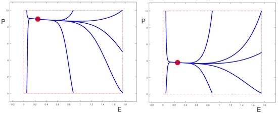
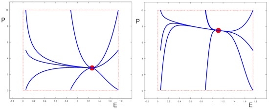
It is clear from Poincaré-Bendixson theory that even if $P_{max,1}<P_{max,2}$, the equilibrium point $(P_{*},E_{*})$ is globally asymptotically stable (in the sense that its region of attraction contains the set ${\mathbb{P}}_0$, and only this region is relevant for the problem) as long as it is the only equilibrium point in ${\mathbb{P}}_0$. This is shown in the phase portraits for the uncontrolled system in Figure 2; Figure 3 shows a case where $P_{max,1}>P_{max,2}$. (The values of the parameters are given in Table 1 and Table 2.) We also show the phase-portraits for the systems when one of the controls is set to be equal to 1 and all others are zero. The two sets of figures illustrate two different scenarios, one where the control parameters are such that the equilibrium can be effectively controlled by all the drugs (Figure 2), the other where it is essentially only the control $u_1$ that is able to move the equilibrium point. However, this behavior depends on the fact that $Q=0$.

Figure 2. Phase portraits of the reduced dynamics for $Q=0$ and $P_{max,1}<P_{max,2}$ for the uncontrolled system (top, left) and for constant controls $u_1\equiv 1$ (top, right), $u_2\equiv 1$ (bottom, left) and $u_3\equiv 1$ (bottom, right). The numerical values for these phase portraits are given in Table 1 and Table 2.

Figure 3. Phase portraits of the reduced dynamics for $Q=0$ and $P_{max,1}>P_{max,2}$ for the uncontrolled system (top, left) and for constant controls $u_1\equiv 1$ (top, right), $u_2\equiv 1$ (bottom, left) and $u_3\equiv 1$ (bottom, right). The numerical values for these phase portraits are given in Table 1 and Table 2.

Since the coefficient $a_1$ is always positive, as $a_0$ vanishes the Jacobian matrix has the eigenvalue 0 and the other eigenvalue is negative. At such a point saddle-node bifurcations arise and two new equilibria, one stable, the other unstable, are born.

Proposition 2.

If $P_{max,2}>P_{max,1}$, then multiple equilibria $(P_{*},E_{*})$ inside ${\mathbb{P}}_0$ can exist. At points $(P_{*},E_{*})$ where

$$\frac{{\delta }_P}{r_P}\frac{\left(P_{max,2}-P_{max,1}\right)P_{*}}{{\left(1+P_{*}+P_{max,1}{P}_{*}\right)}^2}\frac{{\delta }_E}{s_E}\frac{E_{max,2}{E}_{*}}{{\left(1+E_{*}\right)}^2}=1$$

(14)

saddle-node bifurcations occur in which a stable and an unstable equilibrium point merge.

Proof. 

The coefficient $a_0$ vanishes if and only if

$$r_P{s}_E\frac{1+P_{*}+P_{max,1}{P}_{*}}{1+P_{*}}={\delta }_P\frac{E_{max,2}{P}_{*}}{{\left(1+E_{*}\right)}^2}\frac{\left(P_{max,2}-P_{max,1}\right){\delta }_E{E}_{*}}{\left(1+P_{*}\right)\left(1+P_{*}+P_{max,1}{P}_{*}\right)}.$$

This condition is equivalent to (14).

For the underlying biological problem it is natural that an inhibition effect would be smaller than a stimulation effect. Also, the denominators are quadratic in the respective variables E and P, but these variables are scaled. In principle it is possible to satisfy (14), but we did not come across this in our simulations.

3.3. Dynamic Behavior for Positive Q-Values

For the behavior of the overall system, the Q dynamics are essential. If one considers the above equilibria in the plane $Q=0$ now in the full three-dimensional space, then the first row of the Jacobian matrix at $(0,P_{*},E_{*})$ takes the form

$$\left(r_Q-{\delta }_Q\left(1+\frac{E_{max,1}{E}_{*}}{1+E_{*}}\right),0,0\right)$$

and thus $(0,P_{*},E_{*})$ is unstable if $r_Q>{\delta }_Q\left(1+\frac{E_{max,1}{E}_{*}}{1+E_{*}}\right)$ while the local stability properties for the overall system are the same as in the $(P,E)$-plane if $r_Q<{\delta }_Q\left(1+\frac{E_{max,1}{E}_{*}}{1+E_{*}}\right)$. If $r_Q={\delta }_Q\left(1+\frac{E_{max,1}{E}_{*}}{1+E_{*}}\right)$, then there exists a 1-dimensional center manifold (corresponding to the 0 eigenvalue). In this case we have $\dot{Q}=0$ and there exists a curve of equilibria emerging from $(0,P_{*},E_{*})$ parameterized by Q or P (also see below).

Generally, (1)–(3) is a time-varying linear system dominated by exponential growth and decay, depending on the parameter values. If

$$r_Q\ge {\delta }_Q\left(1+E_{max,1}\frac{E_{\mathrm{ss}}}{1+E_{\mathrm{ss}}}\right),$$

then Q grows exponentially and no steady state exists. In this case, the influx $k_{P}Q$ eventually becomes the dominant term in Equation (2) and P also grows beyond limits (Lemma 3). This represents the malignant scenario in the model which corresponds to a highly-aggressive form of the disease or the accelerated or blast phase. The other extreme arises if $r_Q<{\delta }_Q$. In this case Q exponentially decays to 0 for the uncontrolled system and overall trajectories converge to one of the equilibria $(0,P_{*},E_{*})$ in the plane $Q=0$. If there exist multiple such equilibria, there exists a stable manifold for the unstable one that separates the regions of attraction for the stable equilibria. This would reflect a scenario when Q initiates the disease, but eventually dies off and the remaining P population determines the outcome of the disease. This could be benign if $P_{*}$ is small (a form of successful immune surveillance) or malignant if this value is larger. In such a case, however, one only needs to deal with the proliferating cells as far as treatment is concerned. This appears less likely (unless it could be induced by the drugs) and in the uncontrolled case of the disease we would have $r_Q>{\delta }_Q$.

The interesting and most difficult case arises when the uncontrolled system has a chronic steady state or undergoes exponential growth without treatment, but has a negative net growth rate for Q with treatment. This is the case if the parameters satisfy the following condition (A):

$$E_{max,1}\frac{E_{\mathrm{ss}}}{1+E_{\mathrm{ss}}}>\frac{r_Q}{{\delta }_Q}-1>0,$$

(15)

or, with the controls in the original form,

$$E_{max,1}\frac{E_{\mathrm{ss}}}{1+E_{\mathrm{ss}}}\left(1+\frac{U{2}_{max,1}{u}_2}{U2C_{50}+u_2}\right)\left(1+\frac{U{3}_{max,1}{u}_3}{U3C_{50}+u_3}\right)>\frac{r_Q}{{\delta }_Q}-1>0.$$

Thus the replication rate constant $r_Q$ needs to be greater than the death rate constant ${\delta }_Q$ (this naturally will be satisfied for parameters in a disease state), but at the same time, the drugs need to be able to raise the maximum effectiveness ${\widehat{E}}_{max,1}=E_{max,1}\left(1+\frac{U{2}_{max,1}{u}_2}{U2C_{50}+u_2}\right)\left(1+\frac{U{3}_{max,1}{u}_3}{U3C_{50}+u_3}\right)$ high enough that the magnitude of the immune system effect can overcome the difference. These appear to be natural conditions. Assuming that (15) holds, there exists a unique value $E_{*}\in (0,E_{\mathrm{ss}})$ for which $\dot{Q}=0$, namely

$$r_Q={\delta }_Q\left(1+E_{max,1}\frac{E_{*}}{1+E_{*}}\right)⟺E_{*}=\frac{\frac{r_Q}{{\delta }_Q}-1}{E_{max,1}-\left(\frac{r_Q}{{\delta }_Q}-1\right)}$$

(16)

with Q increasing for $E<E_{*}$ and decreasing for $E>E_{*}$. In this case, the interplay between the variables allows for a steady state $(Q_{*},P_{*},E_{*})$ to exist with all values positive. We call such an equilibrium point $(Q_{*},P_{*},E_{*})$ positive.

3.4. Special Case: $P_{max,1}=P_{max,2}$

We first discuss the dynamical behavior of the system for the case $P_{max,1}=P_{max,2}$ which is quite different from the cases $P_{max,1}\ne P_{max,2}$. If these effective rates are equal, we have that

$$\frac{dE}{dt}=\left(s_{E}ln\left(\frac{E_{\mathrm{ss}}}{E}\right)-{\delta }_E\right)\left(1+\frac{P_{max,1}P}{1+P}\right)E$$

and it follows that E is strictly increasing for $E<E_{*}=E_{\mathrm{ss}}exp\left(-\frac{{\delta }_E}{s_E}\right)$ and strictly decreasing for $E>E_{*}$. Therefore, as $t\to \infty$, the E-dynamics approach $E_{*}$, monotonically increasing if the initial condition is smaller, monotonically decreasing if it is higher. Consequently also the Q-dynamics approach the steady-state behavior

$$\frac{dQ}{dt}=\left[r_Q-{\delta }_Q\left(1+\frac{E_{max,1}{E}_{*}}{1+E_{*}}\right)\right]Q$$

and Q will increase exponentially if

$$r_Q>{\delta }_Q\left(1+\frac{E_{max,1}{E}_{*}}{1+E_{*}}\right)$$

and decrease exponentially if

$$r_Q<{\delta }_Q\left(1+\frac{E_{max,1}{E}_{*}}{1+E_{*}}\right).$$

In the first case this also generates unbounded growth in P (Lemma 3) leading to behavior consistent with the blast phase of the system. In the second case, Q decays exponentially to 0 and P converges to the unique and asymptotically stable equilibrium point $P_{*}$ on $Q=0$. Overall, and writing in the constant controls (the respective concentrations $u_i$) we have the following result:

Proposition 3.

Suppose $P_{max,1}=P_{max,2}$ and let

$$\widehat{E}=E_{\mathrm{ss}}exp\left(-\frac{{\delta }_E}{s_E}\right)$$

and

$$\widehat{P}=P_{\mathrm{ss}}exp\left(-\frac{{\delta }_P}{r_P}\left(1+E_{max,2}\frac{\widehat{E}}{1+\widehat{E}}\right)\right).$$

If

$$r_Q<{\delta }_Q\left(1+\left(1+\frac{U{2}_{max,1}{u}_2}{U2C_{50}+u_2}\right)\left(1+\frac{U{3}_{max,1}{u}_3}{U3C_{50}+u_3}\right)\frac{E_{max,1}\widehat{E}}{1+\widehat{E}}\right),$$

then all trajectories $\left(Q\right(t),P(t),E(t\left)\right)$ converge to the unique and asymptotically stable equilibrium point $(0,\widehat{P},\widehat{E})$ in the boundary of ${\mathbb{P}}_0$, whereas if

$$r_Q>{\delta }_Q\left(1+\left(1+\frac{U{2}_{max,1}{u}_2}{U2C_{50}+u_2}\right)\left(1+\frac{U{3}_{max,1}{u}_3}{U3C_{50}+u_3}\right)\frac{E_{max,1}\widehat{E}}{1+\widehat{E}}\right),$$

then Q grows exponentially and ${lim}_{t\to \infty }P\left(t\right)=+\infty$ and ${lim}_{t\to \infty }E\left(t\right)=\widehat{E}$.

If

$$r_Q={\delta }_Q\left(1+\left(1+\frac{U{2}_{max,1}{u}_2}{U2C_{50}+u_2}\right)\left(1+\frac{U{3}_{max,1}{u}_3}{U3C_{50}+u_3}\right)\frac{E_{max,1}\widehat{E}}{1+\widehat{E}}\right),$$

then a positive equilibrium point $(Q_{*},P_{*},E_{*})$ exists, but this relation is non-generic and generally will not be satisfied for a given set of parameters.

3.5. Existence and Stability of a Positive Equilibrium Point $(Q_{*},P_{*},E_{*})$ for $P_{max,1}\ne P_{max,2}$

We analyze whether positive equilibrium points $(Q_{*},P_{*},E_{*})$ exist. Throughout this section we assume that condition (15) is satisfied, i.e., that

$$E_{max,1}\frac{E_{\mathrm{ss}}}{1+E_{\mathrm{ss}}}>\frac{r_Q}{{\delta }_Q}-1>0,$$

since otherwise Q grows exponentially.

Lemma 5.

For $P_{max,1}\ne P_{max,2}$, there exists at most one positive equilibrium point $(Q_{*},P_{*},E_{*})$.

Proof. 

The equilibrium relation for Equation (6) uniquely determines $E_{*}$:

$$r_Q={\delta }_Q\left(1+E_{max,1}\frac{E_{*}}{1+E_{*}}\right)⟺E_{*}=\frac{\frac{r_Q}{{\delta }_Q}-1}{E_{max,1}-\left(\frac{r_Q}{{\delta }_Q}-1\right)}>0.$$

Given $E_{*}$, the equilibrium condition on the effector cells, $\dot{E}=0$, is equivalent to

$$\frac{s_E}{{\delta }_E}ln\left(\frac{E_{\mathrm{ss}}}{E_{*}}\right)=\frac{1+P_{*}+P_{max,2}{P}_{*}}{1+P_{*}+P_{max,1}{P}_{*}}.$$

(17)

The quantity $\frac{s_E}{{\delta }_E}ln\left(\frac{E_{\mathrm{ss}}}{E_{*}}\right)$ is already determined. If $\frac{s_E}{{\delta }_E}ln\left(\frac{E_{\mathrm{ss}}}{E_{*}}\right)=1$, then (17) only has the solution $P_{*}=0$; otherwise there exists a unique solution $P_{*}=P_{*}\left(E_{*}\right)$ given by

$$P_{*}=\frac{1}{1+P_{max,1}}\times \frac{1-\frac{s_E}{{\delta }_E}ln\left(\frac{E_{\mathrm{ss}}}{E_{*}}\right)}{\frac{s_E}{{\delta }_E}ln\left(\frac{E_{\mathrm{ss}}}{E_{*}}\right)-\frac{1+P_{max,2}}{1+P_{max,1}}}.$$

(18)

If $P_{max,1}<P_{max,2}$, this solution is positive if and only if

$$1<\frac{s_E}{{\delta }_E}ln\left(\frac{E_{\mathrm{ss}}}{E_{*}}\right)<\frac{1+P_{max,2}}{1+P_{max,1}}$$

and if $P_{max,1}>P_{max,2}$, the solution is positive if and only if

$$1>\frac{s_E}{{\delta }_E}ln\left(\frac{E_{\mathrm{ss}}}{E_{*}}\right)>\frac{1+P_{max,2}}{1+P_{max,1}}.$$

If one of these inequalities is violated, no positive equilibrium solution $P_{*}=P_{*}\left(E_{*}\right)$ exists and the overall dynamics are determined either by exponential growth or decay of Q. If $P_{*}=P_{*}\left(E_{*}\right)$ exists and is positive, then Equation (7) defines $Q_{*}$ as

$$k_P{Q}_{*}=\left[{\delta }_P\left(1+E_{max,2}\frac{E_{*}}{1+E_{*}}\right)-r_{P}ln\left(\frac{P_{\mathrm{ss}}}{P_{*}}\right)\right]P_{*}.$$

(19)

Using the equilibrium relation for $E_{*}$, this can equivalently be expressed in the form

$$k_P{Q}_{*}=\left[1+\frac{E_{max,2}}{E_{max,1}}\left(\frac{r_Q}{{\delta }_Q}-1\right)-\frac{r_P}{{\delta }_P}ln\left(\frac{P_{\mathrm{ss}}}{P_{*}}\right)\right]{\delta }_P{P}_{*}.$$

(20)

Note that $Q_{*}$ is positive if $P_{*}\ge P_{\mathrm{ss}}$ while otherwise this becomes a requirement on the equilibrium value $P_{*}=P_{*}\left(E_{*}\right)$, namely

$$P_{*}>P_{\mathrm{ss}}exp\left(-\frac{{\delta }_P}{r_P}\left[1+\frac{E_{max,2}}{E_{max,1}}\left(\frac{r_Q}{{\delta }_Q}-1\right)\right]\right).$$

If $E_{max,2}=E_{max,1}$, then this simply becomes $P_{*}>P_{\mathrm{ss}}exp\left(-\frac{{\delta }_P}{r_P}\frac{r_Q}{{\delta }_Q}\right)$. In either case, there exists at most one positive equilibrium point given by Equations (16), (18) and (20).

Remark 1.

As $P_{max,1}\to P_{max,2}$, condition (15) implies that along a positive solution $P_{*}\left(E_{*}\right)$ we must have

$$\frac{s_E}{{\delta }_E}ln\left(\frac{E_{\mathrm{ss}}}{E_{*}}\right)\to 1$$

and thus the limit taken along these positive solutions only exists if $E_{*}\to \widehat{E}=E_{\mathrm{ss}}exp\left(-\frac{{\delta }_E}{s_E}\right)$ and if

$$r_Q={\delta }_Q\left(1+E_{max,1}\frac{\widehat{E}}{1+\widehat{E}}\right).$$

In this degenerate case, the equilibrium conditions $\dot{Q}=0$ and $\dot{E}=0$ are automatically satisfied and there exists a one-dimensional equilibrium manifold, namely $M=\left\{\left(Q_{*}\left(P\right),P,\widehat{E}\right):P>0\right\}$ with the P value arbitrary and $Q_{*}\left(P\right)$ given by

$$Q_{*}\left(P\right)=\frac{1}{k_P}\left[{\delta }_P\left(1+E_{max,2}\frac{\widehat{E}}{1+\widehat{E}}\right)-r_{P}ln\left(\frac{P_{\mathrm{ss}}}{P}\right)\right]P.$$

We now investigate the stability of the positive equilibrium point. The partial derivatives of the equations defining the dynamics at the equilibrium point are given by

$$\begin{array}{cc}\hfill {\frac{\partial f_1}{\partial Q}}_{\left|\right(Q_{*},P_{*},E_{*})}& =0,{\frac{\partial f_1}{\partial P}}_{\left|\right(Q_{*},P_{*},E_{*})}=0,{\frac{\partial f_1}{\partial E}}_{\left|\right(Q_{*},P_{*},E_{*})}=-{\delta }_Q{Q}_{*}\frac{E_{max,1}}{{\left(1+E_{*}\right)}^2},\hfill \\ \hfill {\frac{\partial f_2}{\partial Q}}_{\left|\right(Q_{*},P_{*},E_{*})}& =k_P,{\frac{\partial f_2}{\partial P}}_{\left|\right(Q_{*},P_{*},E_{*})}=-k_P\frac{Q_{*}}{P_{*}}-r_P,{\frac{\partial f_2}{\partial E}}_{\left|\right(Q_{*},P_{*},E_{*})}=-{\delta }_P{P}_{*}\frac{E_{max,2}}{{\left(1+E_{*}\right)}^2},\hfill \\ \hfill {\frac{\partial f_3}{\partial Q}}_{\left|\right(Q_{*},P_{*},E_{*})}& =0,{\frac{\partial f_2}{\partial E}}_{\left|\right(Q_{*},P_{*},E_{*})}=-s_E\left(1+\frac{P_{max,1}{P}_{*}}{1+P_{*}}\right)\hfill \\ \hfill {\frac{\partial f_3}{\partial P}}_{\left|\right(Q_{*},P_{*},E_{*})}& =\frac{s_E{P}_{max,1}ln\left(\frac{E_{\mathrm{ss}}}{E_{*}}\right)-{\delta }_E{P}_{max,2}}{{\left(1+P_{*}\right)}^2}{E}_{*}={\delta }_E{E}_{*}\frac{\left(P_{max,1}-P_{max,2}\right)}{\left(1+P_{*}\right)\left(1+P_{*}+P_{max,1}{P}_{*}\right)}.\hfill \end{array}$$

Note that the equilibrium condition for P brings in $Q_{*}$ in ${\frac{\partial f_2}{\partial P}}_{\left|\right(Q_{*},P_{*},E_{*})}$. The characteristic polynomial for the Jacobian matrix is given by

$$\begin{array}{cc}\hfill \chi \left(t\right)& =\left|\begin{array}{ccc}t& 0& {\delta }_Q{Q}_{*}\frac{E_{max,1}}{{\left(1+E_{*}\right)}^2}\\ -k_P& t+k_P\frac{Q_{*}}{P_{*}}+r_P& {\delta }_P{P}_{*}\frac{E_{max,2}}{{\left(1+E_{*}\right)}^2}\\ 0& {\delta }_E{E}_{*}\frac{P_{max,2}-P_{max,1}}{\left(1+P_{*}\right)\left(1+P_{*}+P_{max,1}{P}_{*}\right)}& t+s_E\left(1+\frac{P_{max,1}{P}_{*}}{1+P_{*}}\right)\end{array}\right|\hfill \\ & =t^3+a_2{t}^2+a_{1}t+a_0.\hfill \end{array}$$

By the Routh-Hurwitz criterion, all eigenvalues have negative real parts if and only if $a_0>0$, $a_1>0$ and $a_1{a}_2>a_0$. These coefficients are given by

$$\begin{array}{cc}\hfill a_2& =\left(k_P\frac{Q_{*}}{P_{*}}+r_P\right)+s_E\left(1+\frac{P_{max,1}{P}_{*}}{1+P_{*}}\right)>0,\hfill \\ \hfill a_1& =\left(k_P\frac{Q_{*}}{P_{*}}+r_P\right)s_E\left(1+\frac{P_{max,1}{P}_{*}}{1+P_{*}}\right)+\frac{E_{max,2}{\delta }_E{E}_{*}}{{\left(1+E_{*}\right)}^2}\frac{\left(P_{max,1}-P_{max,2}\right){\delta }_P{P}_{*}}{\left(1+P_{*}\right)\left(1+P_{*}+P_{max,1}{P}_{*}\right)}\hfill \\ \hfill a_0& ={\delta }_Q{Q}_{*}\frac{E_{max,1}{\delta }_E{E}_{*}}{{\left(1+E_{*}\right)}^2}{k}_P\frac{P_{max,1}-P_{max,2}}{\left(1+P_{*}\right)\left(1+P_{*}+P_{max,1}{P}_{*}\right)}.\hfill \end{array}$$

If $P_{max,1}<P_{max,2}$, then $a_0$ is negative and the positive equilibrium point is unstable, i.e., once the maximal inhibiting effect of the tumor on the effector cells is larger than the maximal stimulating effect, no steady-state positive solution exists. Note further that for $a_0<0$ the characteristic polynomial $\chi \left(t\right)=t^3+a_2{t}^2+a_{1}t+a_0$ has exactly one change of sign in its coefficients and thus there exists a unique positive root. So the equilibrium point has a two-dimensional stable manifold that separates the regions where Q and P diverge to infinity from the region where Q converges to 0. Thus we have the following result:

Theorem 1.

If $P_{max,1}<P_{max,2}$, then the positive equilibrium point $(Q_{*},P_{*},E_{*})$ is unstable with a two-dimensional stable manifold in parameter space.

If $P_{max,1}=P_{max,2}$, then the equilibrium point has the eigenvalue 0 and two negative eigenvalues. Thus there exists a one-dimensional center manifold which in this case consists of all equilibria, namely the equilibrium manifold M defined earlier.

For $P_{max,1}>P_{max,2}$, the coefficients $a_0$, $a_1$ and $a_2$ are all positive. Furthermore

$$\begin{array}{cc}\hfill a_1{a}_2-a_0& =\left[\left(k_P\frac{Q_{*}}{P_{*}}+r_P\right)+s_E\left(1+\frac{P_{max,1}{P}_{*}}{1+P_{*}}\right)\right]\times \hfill \\ & \times \left[\left(k_P\frac{Q_{*}}{P_{*}}+r_P\right)s_E\left(1+\frac{P_{max,1}{P}_{*}}{1+P_{*}}\right)+\frac{E_{max,2}{\delta }_E{E}_{*}}{{\left(1+E_{*}\right)}^2}\frac{\left(P_{max,1}-P_{max,2}\right){\delta }_P{P}_{*}}{\left(1+P_{*}\right)\left(1+P_{*}+P_{max,1}{P}_{*}\right)}\right]\hfill \\ & -{\delta }_Q{Q}_{*}\frac{E_{max,1}{\delta }_E{E}_{*}}{{\left(1+E_{*}\right)}^2}\frac{k_P\left(P_{max,1}-P_{max,2}\right)}{\left(1+P_{*}\right)\left(1+P_{*}+P_{max,1}{P}_{*}\right)}\hfill \\ & >\frac{{\delta }_E{E}_{*}}{{\left(1+E_{*}\right)}^2}\frac{P_{max,1}-P_{max,2}}{\left(1+P_{*}\right)\left(1+P_{*}+P_{max,1}{P}_{*}\right)}{k}_P{Q}_{*}\left({\delta }_P{E}_{max,2}-{\delta }_Q{E}_{max,1}\right).\hfill \end{array}$$

This expression is positive if we make the following assumption (B):

$${\delta }_P{E}_{max,2}\ge {\delta }_Q{E}_{max,1}.$$

(21)

Note from Equations (2) and (3) that ${\delta }_P{E}_{max,2}$ represents the maximal size of the immune effect E on P while ${\delta }_Q{E}_{max,1}$ represents the maximal size of the immune effect E on Q. This effect is assumed to be stronger on the proliferating class of cells than on the quiescent class of cells. Thus assumption (21) is a natural one to make. This assumption is invariant under the actions of the drugs:

$$\begin{array}{cc}\hfill {\widehat{\delta }}_P{\widehat{E}}_{max,2}& =\left(1+\frac{U{1}_{max,2}{u}_1}{U1C_{50}+u_1}\right)\left(1+\frac{U{2}_{max,3}{u}_2}{U2C_{50}+u_2}\right){\delta }_P·\frac{\left(1+\frac{U{2}_{max,1}{u}_2}{U2C_{50}+u_2}\right)\left(1+\frac{U{3}_{max,1}{u}_3}{U3C_{50}+u_3}\right)}{\left(1+\frac{U{1}_{max,2}{u}_1}{U1C_{50}+u_1}\right)\left(1+\frac{U{2}_{max,3}{u}_2}{U2C_{50}+u_2}\right)}{E}_{max,2}\hfill \\ & =\left(1+\frac{U{2}_{max,1}{u}_2}{U2C_{50}+u_2}\right)\left(1+\frac{U{3}_{max,1}{u}_3}{U3C_{50}+u_3}\right){\delta }_P{E}_{max,2}\hfill \end{array}$$

while, letting ${\widehat{\delta }}_Q={\delta }_Q$,

$$\begin{array}{cc}\hfill {\widehat{\delta }}_Q{\widehat{E}}_{max,1}& ={\delta }_Q·\left(1+\frac{U{2}_{max,1}{u}_2}{U2C_{50}+u_2}\right)\left(1+\frac{U{3}_{max,1}{u}_3}{U3C_{50}+u_3}\right)E_{max,1}\hfill \\ & =\left(1+\frac{U{2}_{max,1}{u}_2}{U2C_{50}+u_2}\right)\left(1+\frac{U{3}_{max,1}{u}_3}{U3C_{50}+u_3}\right){\delta }_Q{E}_{max,1}\hfill \end{array}$$

so that these terms are multiplied by the same coefficients. Hence we also have the following result:

Theorem 2.

If $P_{max,1}>P_{max,2}$ and ${\delta }_P{E}_{max,2}\ge {\delta }_Q{E}_{max,1}$, then the positive equilibrium point $(Q_{*},P_{*},E_{*})$ is locally asymptotically stable.

The limiting case $P_{max,1}=P_{max,2}$ represents a degenerate scenario. In many cases no positive equilibrium exists. For example, if $\frac{s_E}{{\delta }_E}ln\left(\frac{E_{\mathrm{ss}}}{E_{*}}\right)\ne 1$, then it follows from (18) that

$$\underset{P_{max,1}\to P_{max,2}}{lim}{P}_{*}=-\frac{1}{1+P_{max,1}}<0.$$

In such a case equilibria will cease to exist, as $P_{max,1}\searrow P_{max,2}$, once the parameter values satisfy

$$1>\frac{s_E}{{\delta }_E}ln\left(\frac{E_{\mathrm{ss}}}{E_{*}}\right)=\frac{1+P_{max,2}}{1+P_{max,1}},E_{*}=\frac{\frac{r_Q}{{\delta }_Q}-1}{E_{max,1}-\left(\frac{r_Q}{{\delta }_Q}-1\right)}.$$

Also, although the positive equilibrium point in Theorem 2 is stable, the value can be very high. In fact, $P_{*}$ diverges to $+\infty$ as these parameter relations are reached (c.f. (18)):

$$P_{*}=\frac{1}{1+P_{max,1}}\frac{1-\frac{s_E}{{\delta }_E}ln\left(\frac{E_{\mathrm{ss}}}{E_{*}}\right)}{\frac{s_E}{{\delta }_E}ln\left(\frac{E_{\mathrm{ss}}}{E_{*}}\right)-\frac{1+P_{max,2}}{1+P_{max,1}}}.$$

For the equilibrium values to be relatively small (‘chronic’), we see that $P_{max,1}$ must be significantly larger than $P_{max,2}$. In terms of the parameter values with drug actions, this can be achieved using the drugs $u_2$ and $u_3$ which increase ${\widehat{P}}_{max,1}$ and decrease ${\widehat{P}}_{max,2}$, c.f.,

$$\begin{array}{cc}\hfill {\widehat{P}}_{max,1}& =\left(1+\frac{U{2}_{max,4}{u}_2}{U2C_{50}+u_2}\right)\left(1+\frac{U{3}_{max,2}{u}_3}{U3C_{50}+u_3}\right)P_{max,1},\hfill \\ \hfill {\widehat{P}}_{max,2}& =\left(1-\frac{U{2}_{max,5}{u}_2}{U2C_{50}+u_2}\right)\left(1-\frac{U{3}_{max,3}{u}_3}{U3C_{50}+u_3}\right)P_{max,2}.\hfill \end{array}$$

So drug administration shifts the balance towards $P_{max,1}$ and this creates an asymptotically stable positive equilibrium point $(Q_{*},P_{*},E_{*})$, hopefully with low values for $P_{*}$ and $Q_{*}$.

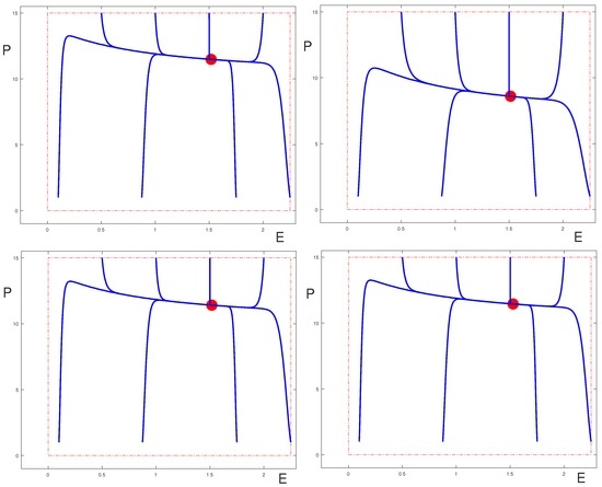
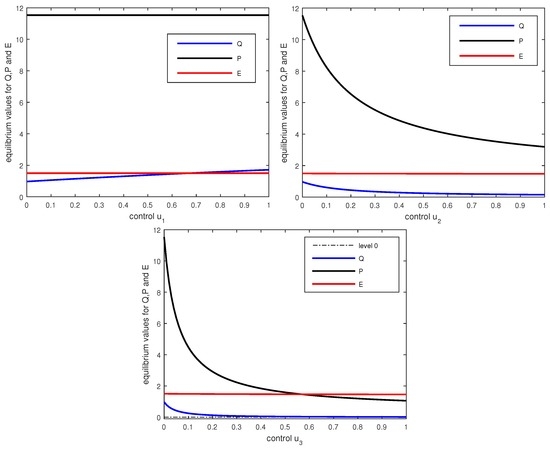
Figure 4 shows how the positive equilibrium values change as (only) one of the controls is varied. Note that the equilibrium values for Q and E do not change if only the control $u_1$ is varied. Also for changes in the controls $u_2$ and $u_3$ these equilibrium values change little and in the graphs the corresponding curves are almost constant. However, in these cases the equilibrium values for Q and P are well-controlled by the therapies. Contrary to the case when $Q=0$, the $u_2$ and $u_3$ controls have strong effects by cutting down the influx of cells from the Q into the P compartment. All equilibria shown in these graphs satisfy the conditions of Theorem 2 and are locally asymptotically stable.

Figure 4. The values of the positive equilibrium point $(Q_{*},P_{*},E_{*})$ as the values for a single control are varied from 0 to 1. The parameter values used in the computations are given in Table 1 and Table 2.

4. Discussion and Conclusions

We considered the dynamical behavior of a mathematical model for CML that incorporated three types of therapies defined by targeted effects on proliferating cells and immunomodulatory properties. We analyzed the long-term dynamical behavior of quiescent and proliferating leukemic cells and immune effects (represented by effector T cells). General parameter values were considered to capture a range of possible scenarios. Some thresholds in the parameter space have been determined analytically that separate different types of dynamical behavior that may correspond to the chronic and the accelerated/blast phases of the disease. It has been illustrated how increasing levels of the therapies affect the equilibrium solutions and their stability. As Q becomes small, the analysis of the dynamics in the plane $Q=0$ indicates that a tyrosine kinase inhibitor can effectively control the disease. However, for larger values of Q, the behavior of the equilibrium solutions shown in Figure 4 suggests that the immunomodulatory properties of the controls $u_2$ and/or $u_3$ are essential in controlling the disease, since $u_1$ alone cannot move the equilibrium value $P_{*}$ if $Q_{*}$ slowly increases. Thus this analysis for constant controls already gives some interesting insights into the roles of the various therapies. Indeed, this analysis for constant parameters and controls is a natural first step towards formulating the model as an optimal control problem where treatment constraints and an objective functional incorporating leukemic cell populations and toxicity for the therapeutic agents will be introduced. Although optimal control solutions such as those computed in [11] can provide insight, optimization of the system under clinical dosing constraints (such as only allowing certain dose levels, and only allowing them to change at certain intervals) would be useful [18].

References

- Faderl, S.; Talpaz, M.; Estrov, Z.; O’Brien, S.; Kurzrock, R.; Kantarjian, H. The biology of chronic myeloid leukemia. N. Engl. J. Med. 1999, 341, 164–172. [Google Scholar] [PubMed]
- Deininger, M.; O’Brien, S.G.; Guilhot, F.; Goldman, J.M.; Hochhaus, A.; Hughes, T.P.; Radich, J.P.; Hatfield, A.K.; Mone, M.; Filian, J.; et al. International randomized study of interferon vs STI571 (IRIS) 8-year follow up: sustained survival and low risk for progression or events in patients with newly diagnosed chronic myeloid leukemia in chronic phase (CML-CP) treated with imatinib. Blood 2009, 114, 1126. [Google Scholar]
- Sawyers, C.L. Chronic myeloid leukemia. N. Engl. J. Med. 1999, 340, 1330–1340. [Google Scholar] [CrossRef] [PubMed]
- Weiden, P.L.; Sullivan, K.L.; Flournoy, N.; Storb, R.; Thomas, E.D.; Seattle Marrow Transplant Team. Antileukemic effect of chronic graft-versus-host disease: Contribution to improved survival after allogeneic marrow transplantation. N. Engl. J. Med. 1981, 304, 1529–1533. [Google Scholar] [CrossRef] [PubMed]
- Talpaz, M.; Kantarjian, H.; McCredie, K.; Trujillo, J.; Keating, M.; Gutterman, J.U. Therapy of chronic myelogenous leukemia. Cancer 1987, 59, 664–667. [Google Scholar] [CrossRef]
- Bristol-Myers Squibb. A Phase 1B Study to Investigate the Safety and Preliminary Efficacy for the Combination of Dasatinib Plus Nivolumab in Patients With Chronic Myeloid Leukemia (CML). Available online: http://clinicaltrials.gov/show/NCT02011945 (accessed on 7 March 2016).
- Rubinow, S.I. A simple model of steady state differentiating cell system. J. Cell Biol. 1969, 43, 32–39. [Google Scholar] [CrossRef] [PubMed]
- Rubinow, S.I.; Lebowitz, J.L. A mathematical model of neutrophil production and control in normal men. J. Math. Biol. 1975, 1, 187–225. [Google Scholar] [CrossRef]
- Fokas, A.S.; Keller, J.B.; Clarkson, B.D. Mathematical model of granulocytopoesis and chronic myelogeneous leukemia. Cancer Res. 1999, 51, 2084–2091. [Google Scholar]
- Moore, H.; Li, N.K. A mathematical model for chronic myelogenous leukemia (CML) and T cell interaction. J. Theor. Biol. 2004, 227, 513–523. [Google Scholar] [CrossRef] [PubMed]
- Nanda, S.; Moore, H.; Lenhart, S. Optimal control of treatment in a mathematical model of chronic myelogenous leukemia. Math. Biosci. 2007, 210, 143–156. [Google Scholar] [CrossRef] [PubMed]
- Moore, H.; Strauss, L.; Ledzewicz, U. Mathematical optimization of combination therapy for Chronic Myeloid Leukemia (CML). In Presented at the 6th American Conference on Pharmacometrics, Crystal City, VA, USA, 4–7 October 2015.
- Afenya, E.K.; Calderón, C. Diverse ideas on the growth kinetics of disseminated cancer cells. Bull. Math. Biol. 2000, 62, 527–542. [Google Scholar] [CrossRef] [PubMed]
- Nakamura-Ishizu, A.; Takizawa, H.; Suda, T. The analysis, roles and regulation of quiescence in hematopoietic stem cells. Development 2014, 141, 4656–4666. [Google Scholar] [CrossRef] [PubMed]
- Gabrielsson, J.; Weiner, D. Pharmacokinetic and Pharmacodynamic Data Analysis: Concepts and Applications, 5th ed.; Apotekarsocieteten: Stockholm, Sweden, 2016. [Google Scholar]
- Shudo, E.; Ribeiro, R.M.; Perelson, A.S. Modelling hepatitis C virus kinetics: the relationship between the infected cell loss rate and the final slope of viral decay. Antivir. Ther. 2009, 14, 459–464. [Google Scholar]
- Branford, S.; Yeung, D.T.; Prime, J.A.; Choi, S.Y.; Bang, J.H.; Park, J.E.; Kim, D.W.; Ross, D.M.; Hughes, T.P. BCR-ABL1 doubling times more reliably assess the dynamics of CML relapse compared with the BCR-ABL1 fold rise: implications for monitoring and management. Blood 2012, 119, 4264–4271. [Google Scholar]
- Schättler, H.; Ledzewicz, U. Optimal Control for Mathematical Models of Cancer Therapies; Springer: New York, NY, USA, 2015. [Google Scholar]
© 2016 by the authors; licensee MDPI, Basel, Switzerland. This article is an open access article distributed under the terms and conditions of the Creative Commons Attribution (CC-BY) license (http://creativecommons.org/licenses/by/4.0/).