Monte Carlo Simulation-Based Robustness Analysis of High-Speed Railway Settlement Prediction Models for Non-Stationary Time Series

Abstract

Accurate prediction of post-construction settlement in high-speed railway (HSR) soft foundations is critical for operational safety yet challenging due to the non-equidistant and non-stationary nature of observation data. This study systematically evaluated the robustness and accuracy of settlement prediction models using a Monte Carlo simulation approach. A numerical model incorporating the permeability characteristics of soft foundations was established to simulate stochastic system responses. Furthermore, an innovative multi-metric evaluation framework was constructed using the entropy weight method, integrating goodness-of-fit, prediction accuracy (systematic error), and stability (random error). Four classical empirical models—Hyperbolic, Exponential Curve, Asaoka, and Hoshino—were assessed. The results indicate that: (1) The Hyperbolic Method significantly outperformed other models ($p<0.01$) in goodness-of-fit (mean correlation coefficient: 0.983 ± 0.006) and accuracy (systematic error: 3.2% ± 1.1%); (2) The Hoshino Method exhibited optimal stability, characterized by the lowest random error (3.8 ± 2.0 mm); and (3) Model performance showed a significant positive correlation with the permeability coefficient ($R^2>0.92$). Validated by five distinct engineering cases, the comprehensive performance ranking was determined as: Hyperbolic > Hoshino > Exponential Curve > Asaoka. These findings provide a scientific strategy for model selection under non-stationary conditions and offer theoretical support for refining railway deformation monitoring standards.

1. Introduction

1.1. Background and Motivation

The smoothness of high-speed railway (HSR) track structures is intrinsically linked to the precise control of post-construction settlement in subgrades. This remains a paramount challenge in the construction and maintenance of modern railway infrastructure [1,2]. In engineering practice, settlement control typically relies on a combination of theoretical calculations and empirical prediction models. However, theoretical approaches, such as the traditional layered summation method, often yield significant computational errors [3]. This is particularly evident in soft foundations characterized by high compressibility ($a=1.5–2.4{ \mathrm{MPa}}^{-1}$), low permeability ($K={10}^{-4}–{10}^{-3} \mathrm{m}/\mathrm{d}$), and pronounced rheological properties [4,5,6]. While refined numerical simulations offer alternatives, they are frequently hindered by low computational efficiency and the difficulty of accurate parameter determination [7]. Consequently, establishing accurate theoretical control is exceptionally difficult, rendering settlement prediction a critical safeguard for ensuring track regularity.

The efficacy of settlement prediction is fundamentally determined by the quality of observational data, which dictates the system response—specifically, the accuracy and stability—of prediction models. However, HSR settlement data inherently exhibit complex characteristics. First, the observation frequency varies drastically across different construction phases (e.g., filling, static loading), leading to non-equidistant data sequences [8,9]. Second, the data contain both genuine time-varying settlement trends and random noise arising from measurement errors, environmental factors, and construction conditions, resulting in non-stationary properties (i.e., time-varying statistical characteristics) [10,11]. The coupling of these non-equidistant and non-stationary features poses a severe threat to the robustness and reliability of prediction models [12].

1.2. Challenges and Research Gaps

Despite the critical nature of this problem, existing research faces significant limitations in data preprocessing, model evaluation, and the understanding of coupled data effects.

To address data irregularities, researchers have employed various interpolation and denoising techniques. Regarding non-equidistant data, methods such as cubic spline interpolation [13], Piecewise Cubic Hermite Interpolating Polynomials (PCHIP) [14], and hybrid neural network approaches [15] have been utilized. Similarly, for non-stationary data, techniques including Wavelet Transform (WT) [16], Kalman Filtering (KF) [17], Empirical Mode Decomposition (EMD) [18], and multi-stage hybrid denoising [19] have shown promise in specific scenarios. However, traditional interpolation often distorts the true time-varying characteristics of settlement, while advanced machine learning methods [20,21] require extensive training datasets and lack physical consistency, limiting their practical application in engineering projects with sparse samples. Furthermore, these methods typically address non-equidistant and non-stationary properties in isolation, failing to account for their interaction.

Current evaluation standards, both in China and internationally, predominantly rely on single metrics. For instance, German railway authorities [22] and Chinese standards [8,9] emphasize goodness-of-fit metrics like the coefficient of determination ($R^2\ge 0.85$) or correlation coefficient ($r\ge 0.92$). However, scholars argue that $R^2$ is potentially misleading for nonlinear regression [23]. While some studies have introduced error-based metrics such as Mean Squared Error (MSE), Mean Absolute Percentage Error (MAPE), or absolute error [24,25,26,27,28], these single-dimension indicators cannot comprehensively capture the multifaceted requirements of HSR settlement control.

Although the individual impacts of data irregularities have been explored, the quantitative mechanisms of the coupled effects of non-equidistant and non-stationary data on model robustness remain unclear. There is a distinct lack of a systematic framework that can effectively quantify these coupled effects and integrate multidimensional performance metrics (goodness-of-fit, accuracy, and stability) through objective weighting. Addressing this gap is essential for selecting robust prediction models in complex engineering environments.

1.3. Contributions and Objectives

To bridge these gaps, this study proposes a robust prediction strategy and a novel evaluation system for HSR soft foundation settlement. The primary contributions and objectives are as follows:

• Quantification of Coupled Effects via Monte Carlo Simulation: Unlike previous studies that treat data issues separately, this research utilizes Monte Carlo simulation to systematically investigate and quantify the impact mechanisms of coupled non-equidistant and non-stationary time series data on the system response of prediction models.
• Development of a Multi-Metric Evaluation Framework: We construct a comprehensive evaluation framework that integrates goodness-of-fit, prediction accuracy (systematic error), and stability (random error). By employing the Entropy Weight Method, this framework objectively assigns weights to each metric, overcoming the bias inherent in single-metric evaluations.
• Validation and Model Selection Strategy: Through numerical experiments and cross-validation with five typical engineering cases, this study evaluates four mainstream empirical models (Hyperbolic, Exponential Curve, Asaoka, and Hoshino). The results provide a scientific, evidence-based strategy for model selection and offer theoretical support for revising railway deformation observation standards.

2. Theoretical Framework and Methodology

2.1. Development of the Settlement Prediction Numerical Model

To systematically investigate the robustness of settlement prediction models, this study establishes an integrated analytical framework that synergizes theoretical consolidation modeling with Monte Carlo-based numerical simulation. The technical roadmap is illustrated in Figure 1. The framework is structured into three progressive phases:

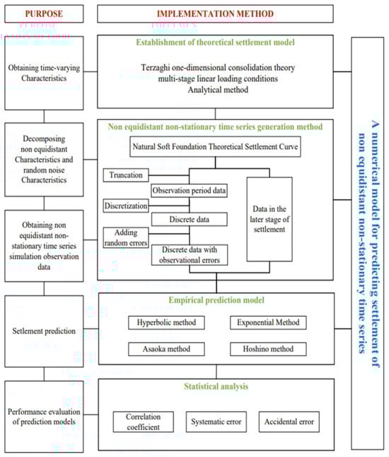
Figure 1. Technical Roadmap.

Phase 1: Baseline Settlement Model: First, a baseline settlement model is constructed based on Terzaghi’s one-dimensional consolidation theory, explicitly accounting for the multi-stage loading conditions typical in high-speed railway construction. Validation against in situ monitoring data confirms the model’s high computational fidelity, with relative errors maintained below 1%, ensuring a reliable physical basis for subsequent simulations.

Phase 2: Monte Carlo Data Generation Protocol: Second, to address the challenges posed by observational data quality, a novel data generation protocol is developed using Monte Carlo simulation. This approach replicates the stochastic nature of field measurements, specifically targeting non-equidistant sampling and non-stationary noise. As detailed in Section 2.2, the protocol implements a sequential workflow: (i) theoretical curve truncation, (ii) non-equidistant discretization, and (iii) random noise superposition. This methodology effectively decouples deterministic time-varying trends from stochastic noise, generating large-scale synthetic datasets ($N={10}^4$ samples per scenario) that statistically mirror the complexities of engineering reality.

Phase 3: Comparative Performance Assessment: Finally, a comparative performance assessment is conducted on four standard empirical models: the Hyperbolic Method, Exponential Curve Method, Asaoka Method, and Hoshino Method. Utilizing a control variable strategy, extensive Monte Carlo iterations are performed to statistically quantify critical performance metrics, including correlation coefficients, systematic errors, and random errors. These quantitative results establish the data foundation for the multi-metric evaluation framework proposed in this study.

2.1.1. Theoretical Formulation of Subgrade Settlement

The governing equations of the model are given in Appendix A, Equation (A1), and detailed derivations, boundary conditions, and solution procedures are also provided in Appendix A.

2.1.2. Method for Generating Non-Equidistant and Non-Stationary Time Series

To systematically evaluate model robustness under realistic monitoring conditions, this study proposes a stochastic data generation framework based on Monte Carlo simulation. Unlike traditional methods that rely on static datasets, this framework enables the quantitative decoupling and parametric control of three critical components inherent in field observations: (i) Generation of Theoretical Baseline, (ii) Non-Equidistant Discretization, (iii) Stochastic Measurement Noise, (iv) Stochastic Noise Injection. By independently manipulating these parameters, the method generates synthetic datasets that statistically mirror complex engineering realities. The generation protocol proceeds through the following sequential steps:

Step 1: Generation of Theoretical Baseline

The analytical solution derived in Section 2.1.1 (Appendix A, Equations (A13) and (A15)) is utilized to generate the continuous theoretical settlement curve, $S\left(t\right)$. This curve represents the “true” physical response of the subgrade under ideal, noise-free conditions.

Step 2: Temporal Partitioning (Truncation)

To simulate realistic prediction scenarios, the continuous timeline is partitioned into two distinct phases based on the observation duration: the monitoring window ($0\le t\le t_{obs}$) and the prediction horizon ($t>t_{obs}$). As illustrated in Figure 2a, only the data within the monitoring window are retained for model fitting, while the subsequent data serve as the ground truth for validation.

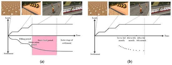
Figure 2. Schematic Diagram of Non-Equidistant and Non-Stationary Time Series Simulation and Observational Data Generation: (a) Theoretical Curve Truncation; (b) Non-Equidistant Discretization [29].

Step 3: Non-Equidistant Discretization

The continuous data within the monitoring window are discretized to replicate irregular field sampling schedules. As shown in Figure 2b, sampling points are selected based on non-uniform time intervals (e.g., varying frequencies across different construction stages), transforming the continuous curve into a discrete, non-equidistant sequence.

Step 4: Stochastic Noise Injection

To emulate non-stationary measurement errors and environmental perturbations, random noise is superimposed onto the discretized observation points. this process generates a massive volume of synthetic observational datasets ($N={10}^4$) characterized by both sampling irregularity and stochastic noise, providing a rigorous database for the subsequent Monte Carlo robustness analysis.

This study adopted the independent and identically distributed normal distribution as the assumption for random noise. On the one hand, according to the Central Limit Theorem, when random errors result from the superposition of multiple independent factors, their distribution tends to approximate a normal distribution. On the other hand, in the absence of specific prior distribution information from engineering practice, the normal distribution, as the most commonly used random distribution assumption, allows for effective control of noise intensity through the standard deviation parameter. This facilitates the quantitative analysis of the impact of non-stationary characteristics on the models. However, we acknowledge that this simplification may not fully capture the noise characteristics under certain specific working conditions. Future research will introduce more complex noise models (such as skewed distributions or autocorrelated noise) to further validate the generalization capability of the models, thereby enhancing the applicability of the prediction system in practical engineering.

2.1.3. Objective Function of Prediction Models

The fitting parameters for empirical prediction models, including the Hyperbolic Method [30], Exponential Curve Method [31], Asaoka Method [32], and Hoshino Method [33,34], are determined based on the least squares principle [35]. The objective function is formulated as Equation (1), illustrated in Figure 3:

$$\arg \min E={\displaystyle \sum _{i=1}^n{(y_i-{\stackrel{⌢}{y}}_i)}^2}$$

(1)

where $n$ is the number of simulated observational data point; $y_i$ is the observed value from simulated data; ${\stackrel{⌢}{y}}_i$ is the fitted value calculated by the respective empirical model.

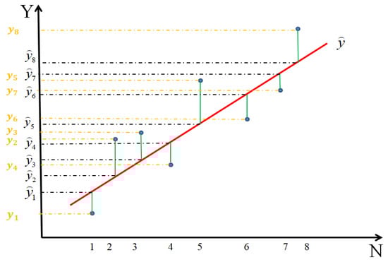
Figure 3. Schematic Diagram of Least Squares Principle.

In this study, a Monte Carlo-based simulation framework was employed to assess the reliability of the four empirical models under uncertainty. As shown in Figure 4a, the models were applied to large-scale synthetic observational data characterized by non-equidistant sampling intervals and non-stationary trends, with varying degrees of random noise introduced to simulate real-world monitoring environments. Equation (2) is shown below:

$$r={\displaystyle \frac{Cov(\overline{X},\overline{Y})}{\sqrt{D(\overline{X})}·\sqrt{D(\overline{Y})}}}$$

(2)

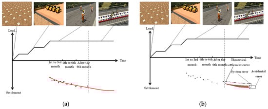
Figure 4. Statistical Analysis of Results: (a) Repeated Settlement Predictions; (b) Statistical Analysis of Results [29].

The statistical distribution of the prediction results is visualized in Figure 4b. To comprehensively evaluate model performance, the total prediction error was decomposed into two distinct components. Equations (3)–(5) are shown below:

$$\mu ={\displaystyle \frac{1}{N_s}}{\displaystyle \sum _{k=1}^{N_s}{S}_k}$$

(3)

$$\overline{x}=\mu -{S_{\infty }}^{\prime }$$

(4)

$$\delta =\overline{x}/{S_{\infty }}^{\prime }$$

(5)

Systematic Error (Measure of Accuracy): This metric quantifies the model’s tendency to consistently overestimate or underestimate the target. It is defined as the discrepancy between the statistical mean of the predicted final settlement (calculated via Equation (3)) and the true theoretical settlement value (derived from Equations (4) and (5)). A lower systematic error indicates higher prediction accuracy [25,26].

Random Error (Measure of Stability): This metric assesses the dispersion of prediction results caused by data noise. It is mathematically represented by the standard deviation of the predicted final settlement (Equation (6)). A smaller standard deviation implies that the model is robust and less sensitive to fluctuations in the input data, thereby reflecting higher stability.

$$\sigma =\sqrt{{\displaystyle \frac{1}{N_s-1}}{\displaystyle \sum _{k=1}^{N_s}{[S_k-\mu ]}^2}}$$

(6)

where $r$ is the correlation coefficient; $Cov(\overline{X},\overline{Y})$ is the covariance between two data series; $D(\overline{X})$ and $D(\overline{Y})$ are the variance of two data series; $\mu$ is the predicted mean of settlement; $\overline{x}$ is the absolute error of settlement prediction; $\delta$ is the relative error of settlement prediction; ${S_{\infty }}^{\prime }$ is the theoretical final settlement; $\sigma$ is the standard deviation of settlement prediction; $N_s$ is the sample size per observation; $S_k$ is the predicted final settlement in the k-th iteration.

2.2. Numerical Simulation Setup

To verify the validity and applicability of the proposed theoretical model, field monitoring data reported by Du Mingfang et al. [36] under complex multi-stage loading conditions were utilized as a benchmark. As illustrated in Figure 5, the settlement trajectory calculated by the theoretical model demonstrated high consistency with the in situ measured data throughout the consolidation process. A quantitative comparison revealed that at the 90-day mark of static loading, the calculated settlement was 115 cm against a field measurement of 116 cm. This resulted in a relative error of merely 0.86%, which falls well within the acceptable range for engineering computational analysis. These findings confirm that the established numerical model effectively captures the settlement behavior of soft foundations.

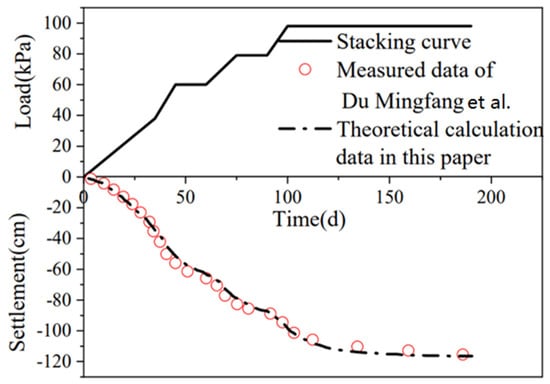
Figure 5. Validation of Theoretical Calculation Results, Du Mingfang et al. [36].

The accuracy of Monte Carlo simulations inherently improves as the sample size increases; however, this comes at the cost of significantly higher computational resources and extended calculation times. To balance computational efficiency with prediction precision, a convergence test was conducted to determine the minimum sample size required for the numerical model. The case study by Du Mingfang et al. [36] was utilized as the baseline scenario.

(1) Convergence Test for Predicted Settlement Means

The simulation setup was consistent with the static loading phase of the case study (commencing from Day 96). A non-equidistant observation scheme was adopted to mimic real-world monitoring: weekly observations for the first three months (1st–3rd month) and bi-weekly observations for the subsequent three months (4th–6th month), totaling 20 observation points over a 6-month period. Random noise was injected into the generated data in accordance with Grade III [37] observation accuracy standards.

To evaluate convergence, single-batch sample sizes ranging from 10 to 200 were tested (corresponding to a total simulated volume of 200–6000 runs). A massive-scale simulation (single-sample size = $1\times {10}^5$, total samples = $2\times {10}^6$) served as the “True Value” benchmark. The predicted mean settlements of the four empirical models (Hyperbolic, Exponential, Asaoka, and Hoshino) were compared against this benchmark, as shown in Figure 6a.

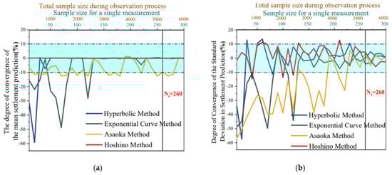
Figure 6. Monte Carlo Simulation Convergence Test: (a) Results of Settlement’s Predicted Mean Convergence Test; (b) Results of Predicted Settlement Standard Deviation Convergence Test.

Adopting a relative deviation threshold of ≤10% [38] as the convergence criterion, distinct behaviors were observed. At small sample sizes, the Hyperbolic and Exponential Curve methods exhibited significant fluctuations, indicating high sensitivity to sampling quantity. However, these fluctuations diminished rapidly as the sample size increased. In contrast, the Asaoka and Hoshino methods demonstrated high stability, with predicted means showing minimal sensitivity to sample size changes. When the single-sample size reached 260, the fluctuations for all models stabilized within the control criterion, balancing accuracy and efficiency.

Using the same methodology, the standard deviations of predicted settlements were tested. Results are shown in Figure 6b. Using a deviation rate ≤ 10% [38] as the control criterion, when the single-sample size was small, the predicted settlement standard deviations from Hyperbolic Method, Exponential Curve Method, and Asaoka Method exhibited significant fluctuations. As the sample size increases, the fluctuations in these three empirical models’ standard deviations decreased markedly. In contrast, the fluctuation of the Hoshino Method’s predicted standard deviation showed minimal correlation with the sample size. When the single-sample size reached $N_s\ge 260$, the fluctuations in predicted standard deviations for all empirical models were well-controlled.

The minimum single-sample size for all empirical models was determined as $N_s\ge 260$, ensuring computational accuracy (deviation rate ≤ 10%). This sample size was adopted in subsequent analyses.

2.3. The Multi-Metric Evaluation Framework

Deformation monitoring for high-speed railway subgrades demands distinct performance metrics from empirical prediction models. These include exceptional fitting capability to capture settlement evolution, high precision in forecasting final settlement to satisfy safety controls, and superior stability to resist noise in non-equidistant and non-stationary datasets. Therefore, model selection constitutes a classic multi-criteria decision-making (MCDM) problem.

In this study, the Entropy Weight Method (EWM) was utilized to resolve this multi-objective challenge [39,40]. The EWM is preferred for its ability to determine weights based solely on the intrinsic dispersion of the indicators. This data-driven approach guarantees mathematical rigor and effectively mitigates the subjective bias often associated with expert scoring methods [41]. The stepwise construction of the comprehensive evaluation index via EWM is detailed below:

Step 1. Construct a judgment matrix A with $p$ alternatives (four empirical models) and $q$ evaluation indicators (correlation coefficient, systematic error, random error);

Step 2. Normalize the judgment matrix to obtain matrix B: Equation (7) is shown below:

$$B=(b_{ij})={\displaystyle \frac{x_{ij}-x_{\min }}{x_{\max }-x_{\min }}}(i=1,2,\dots ,q;j=1,2,\dots ,p)$$

(7)

where $x_{\max }$ and $x_{\min }$ are the maximum and minimum values.

Step 3. Calculate the entropy of each indicator; Equations (8) and (9) are shown below:

$$H_i=-{\displaystyle \frac{1}{\ln p}}\left[{\displaystyle \sum _{j=1}^p(f_{ij}\cdot \ln f_{ij})}\right],(i=1,2,\dots ,q;j=1,2,\dots ,p)$$

(8)

$$f_{ij}={\displaystyle \frac{b_{ij}}{{\displaystyle \sum _{j=1}^p{b}_{ij}}}}$$

(9)

Step 4. Determine the entropy weight, Equations (10) and (11) is shown below:

$$W={({\omega }_i)}_{1\times q}$$

(10)

$${\omega }_i={\displaystyle \frac{1-H_i}{q-{\displaystyle \sum _{i=1}^q{H}_i}}}, \mathrm{and} {\displaystyle \sum _{i=1}^q{\omega }_i}=1$$

(11)

Step 5. Repeat Steps 1–4 for cases with permeability coefficients ranging from K = 2.76 × 10⁻⁴ m/d to 13.6 × 10⁻⁴ m/d, then compute the average entropy weights. The final comprehensive evaluation index is, Equation (12) is shown below:

$$\chi =0.310\times r^n+0.287\times (1-{\delta }^n)+0.403\times (1-{\sigma }^n)$$

(12)

where $r^n$, ${\delta }^n$, ${\sigma }^n$ are the normalized correlation coefficient, systematic error, and random error, respectively.

2.4. Overview of Engineering Cases

(1)

Engineering Background

The selected case study is a 37-m section of the Lanzhou–Lianyungang Railway [42]. The embankment height (3.0–3.6 m) approaches the critical height (3.8–3.9 m). The soft foundation remains untreated, but stability was enhanced using double-layer geotextiles and counterweight berms. Key design parameters included a consolidation degree ($U$) of 20% and a safety factor ($F_s$) of 1.16. The construction featured a rapid filling cycle (2–4 months) without a static loading period.

(2)

Geological Characteristics

The site is located in the Lianyungang Plain, underlain by a 0–12 m thick layer of marine-deposited soft clay. The soil presents typical rheological characteristics of soft marine deposits, including high water content ($w$ = 65.9–78.1%), high compressibility ($a$ = 1.66–2.4 MPa⁻¹), and low shear strength ($q_u$ = 2.33–5.07 kPa). Hydraulic properties are poor, with low permeability ($K\approx {10}^{-3}$ m/d) and a low consolidation coefficient ($C_v\approx {10}^{-4}$ cm²/s). The soil exhibits medium-high sensitivity. ($S_t$ = 2–6) with uniform stratification. Figure 7 illustrates the depth-dependent distribution of these soil parameters.

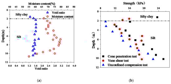
Figure 7. Distribution Patterns of Soil Parameters with Depth: (a) Distribution of Void Ratio and Water Content; (b) Distribution of Comprehensive Strength.

Settlement magnitudes are closely related to soft soil thickness. As shown in Figure 8a, severe settlement areas (e.g., K13–K15 sections) correspond to the thickest soft soil layers and thinnest hard crust layers. The settlement-load–time curves for typical cross-sections in these areas are illustrated in Figure 8b.

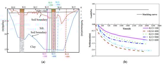
Figure 8. Deformation Observation Data: (a) Relationship Between Soft Soil Thickness and Subgrade Settlement; (b) Settlement-Load–Time Curve for a Typical Cross-Section.

3. Result

3.1. Simulation Results: Accuracy and Stability

(1)

Variation Patterns of Correlation Coefficients

Figure 9 presents the bar chart of correlation coefficients for the empirical prediction models. For the Hyperbolic Method, the correlation coefficient remained ≥0.98 across all permeability conditions, indicating its strong capability to describe the time-varying characteristics of settlement. For the Exponential Curve Method, the correlation coefficient decreased gradually as the permeability coefficient increased. When K < 11.4 × 10⁻⁴ m/d, the coefficient declined significantly, dropping below 0.94 at K > 13.6 × 10⁻⁴ m/d. This suggests that the Exponential Curve Method is more suitable for soft foundations with lower permeability. For the Asaoka Method, the correlation coefficient increased with higher permeability coefficients. When K < 2.76 × 10⁻⁴ m/d, the coefficient remained <0.92, indicating limited applicability to low-permeability soft foundations. For the Hoshino Method, similar to the Asaoka Method, the correlation coefficient improved with increasing permeability. However, when K < 2.76 × 10⁻⁴ m/d, the coefficient remained <0.96, highlighting its dependency on higher permeability for optimal performance.

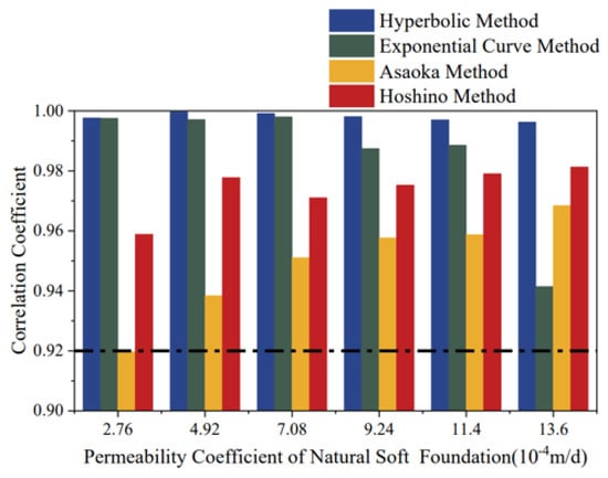
Figure 9. Bar Chart of Correlation Coefficients for Empirical Prediction Models.

(2)

Variation Patterns of Systematic Error and Random Error

Systematic errors in prediction results were evaluated using relative error, while random errors were assessed using the standard deviation of settlement predictions (Equation (5)). As shown in Figure 10 and Figure 11, both systematic and random errors of the four empirical models decreased rapidly with increasing permeability coefficient, following a power function relationship. For soft foundations with lower permeability, both prediction accuracy and stability were relatively poor; however, they improved significantly as the permeability increased. This occurs because under identical observation duration, frequency, and accuracy conditions, soft foundations with higher permeability exhibit a greater degree of settlement completion. The time-varying characteristics of the observed data become smoother, reducing the fitting difficulty of empirical models and thereby enhancing prediction accuracy. These findings are consistent with statistical data reported by Kliesch K and Liu [23,29]. Consequently, accelerating drainage consolidation in soft foundation treatment can effectively improve the quality of deformation monitoring and evaluation.

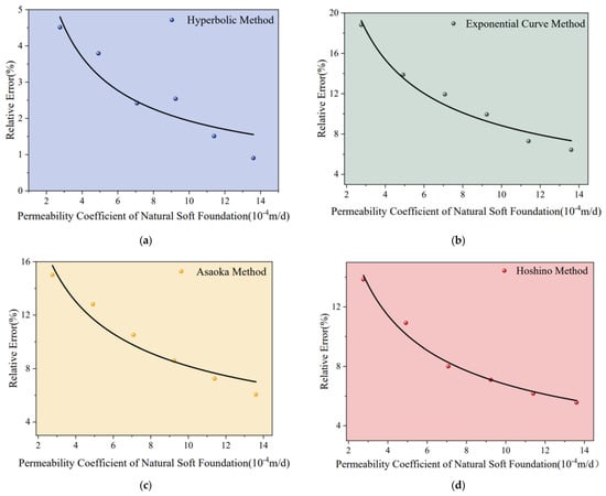
Figure 10. Scatter Plots of Systematic Errors Under Different Permeability Coefficients: (a) Hyperbolic Method; (b) Exponential Curve Method; (c) Asaoka Method; (d) Hoshino Method.

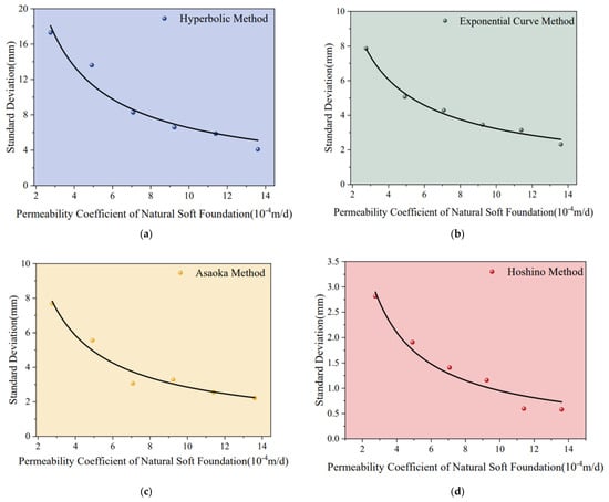
Figure 11. Scatter Plots of Random Errors Under Different Permeability Coefficients: (a) Hyperbolic Method; (b) Exponential Curve Method; (c) Asaoka Method; (d) Hoshino Method.

In terms of magnitude, as shown in Figure 12, the systematic errors of the four empirical models differed significantly. Overall, the ranking was: Exponential Curve Method > Asaoka Method > Hoshino Method > Hyperbolic Method. This indicates that the Hyperbolic Method had the best prediction accuracy, the Exponential Curve Method had the poorest accuracy, while Asaoka Method and Hoshino Method exhibited moderate accuracy.

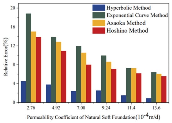
Figure 12. Bar Chart of Systematic Errors for Empirical Prediction Models.

In terms of magnitude, as shown in Figure 13, the random errors of the four empirical models differed significantly. Overall, the ranking was: Hyperbolic Method > Exponential Curve Method ≈ Asaoka Method > Hoshino Method. This indicates that the Hoshino Method had the best stability, Hyperbolic Method had the poorest stability, while the Exponential Curve Method and Asaoka Method exhibited moderate stability.

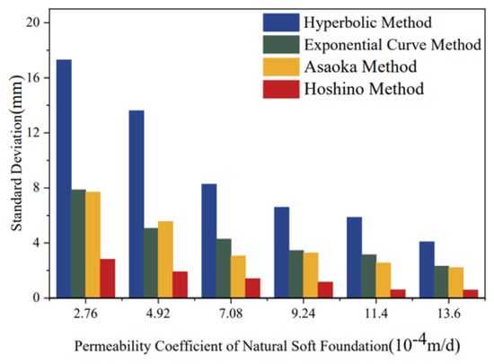
Figure 13. Bar Chart of Random Errors for Empirical Prediction Models.

The above analysis demonstrates that the Hyperbolic Method exhibits strong fitting capability for time-varying settlement curves and high prediction accuracy but poorer stability. The Exponential Curve Method is less effective in describing time-varying characteristics of high-permeability soft foundations, with lower accuracy but better stability. The Asaoka Method is unsuitable for low-permeability soft foundations but provides balanced accuracy and stability. The Hoshino Method ranked second in fitting capability, improved with higher permeability, and offered the best stability (Table 1).

Table 1. Empirical Prediction Models’ Aggregation Results.

Models	Goodness-of-Fit (Correlation Coefficient)	Prediction Accuracy (Systematic Error) (%)	Prediction Stability (Random Error) (mm)
Hyperbolic Method	0.983 ± 0.006	3.2 ± 1.1	>6
Exponential Curve Method	0.91 ± 0.03	13.65 ± 5.35	6.4 ± 3.2
Asaoka Method	0.92 ± 0.02	10.05 ± 3.95	6.4 ± 2.5
Hoshino Method	0.94 ± 0.02	7.65 ± 3.75	3.8 ± 2.0

3.2. Comprehensive Ranking Results

Figure 14 shows the bar chart of comprehensive evaluation indices for the Hyperbolic Method, Exponential Curve Method, Asaoka Method, and Hoshino Method. In terms of trends, the comprehensive evaluation indices of all four empirical models increased with higher permeability coefficients. The performance of the models was higher for soft foundations with better drainage capacity and lower for those with weaker drainage capacity.

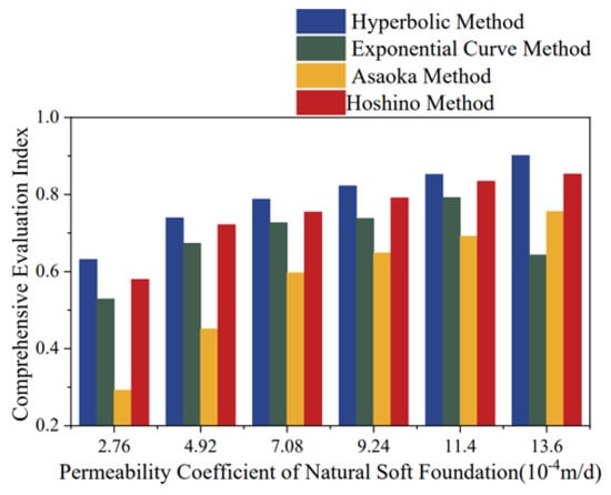
Figure 14. Bar Chart of Comprehensive Evaluation Indices for Empirical Prediction Models.

In terms of magnitude, under different permeability conditions, the comprehensive performance ranking of the models was: Hyperbolic Method > Hoshino Method > Exponential Curve Method > Asaoka Method. For natural soft foundation conditions, the Hyperbolic Method delivered the optimal prediction results, followed by the Hoshino Method, while the Exponential Curve Method and Asaoka Method exhibited poorer performance.

To verify the robustness of the weights derived from the Entropy Weight Method (with goodness-of-fit at 31.0%, accuracy at 28.7%, and stability at 40.3%), we conducted a weight perturbation experiment. We systematically adjusted the weights of each indicator within a ±20% range and observed changes in the rankings of the models’ comprehensive scores. The results (Table 2) indicate that under balanced weight conditions, the ranking order of the four different prediction models remained identical to that under the benchmark weights. When the weighting scheme placed greater emphasis on stability—specifically, when the weight assigned to random error was set to 50%—the Hoshino method rose to the top rank. This finding further underscores that the Hoshino method exhibits stronger stability in its prediction outcomes.

Table 2. Model Ranking Table under Different Weight Combinations.

Alternative Weighting Scenarios	Hyperbolic Method	Exponential Curve Method	Asaoka Method	Hoshino Method	Ranking Changes
Control Weights (31.0%, 28.7%, 40.3%)	0.82	0.72	0.61	0.60	Standard
Balanced Weights (33.3%, 33.3%, 33.3%)	0.79	0.75	0.63	0.62	Unchanged
Stability-focused (25%, 25%, 50%)	0.76	0.78	0.58	0.59	Hoshino Method No.1

3.3. Field Validation Results

The Hyperbolic Method, Exponential Curve Method, Asaoka Method, and Hoshino Method were applied to predict the settlement curves of this case. The correlation coefficients, systematic errors, random errors, and comprehensive evaluation indices are summarized in Table 3. The Hyperbolic Method achieved the highest comprehensive evaluation indices at K13+100, K13+200, K13+600, and K13+900, see Figure 15a–d, demonstrating optimal performance, while the Hoshino Method ranked second in most sections but showed the best performance at K14+400, see Figure 15e. For the Exponential Curve Method and Asaoka Method, they exhibited lower comprehensive evaluation indices across all sections compared to the Hyperbolic and Hoshino Methods. The case study confirms that the comprehensive performance ranking of the models for natural soft foundations is: Hyperbolic Method > Hoshino Method > Asaoka Method ≈ Exponential Curve Method, consistent with the theoretical analysis.

Table 3. Prediction Results of Empirical Models.

Mileage	Model	Correlation Coefficient	Systematic Error (%)	Random Error (mm)	Comprehensive Index
K13+100	Hyperbolic Method	0.95	3.5	6.3	0.74
	Exponential Curve Method	0.93	12	3.7	0.60
	Asaoka Method	0.92	9.3	4.1	0.61
	Hoshino Method	0.92	8	1	0.72
K13+200	Hyperbolic Method	0.93	6	10.3	0.52
	Exponential Curve Method	0.88	19	7.7	0.21
	Asaoka Method	0.9	14	6.1	0.41
	Hoshino Method	0.91	11.4	5.6	0.50
K13+600	Hyperbolic Method	0.96	2.8	5.2	0.82
	Exponential Curve Method	0.94	8.3	3.2	0.72
	Asaoka Method	0.93	6.1	3.9	0.70
	Hoshino Method	0.92	3.9	1.8	0.77
K13+900	Hyperbolic Method	0.97	5.6	10.2	0.66
	Exponential Curve Method	0.92	6.3	7.1	0.58
	Asaoka Method	0.94	7.1	8.3	0.59
	Hoshino Method	0.94	7.9	5.8	0.65
K14+400	Hyperbolic Method	0.98	7.4	15.2	0.52
	Exponential Curve Method	0.9	13.3	9.6	0.32
	Asaoka Method	0.92	10.9	8.9	0.45
	Hoshino Method	0.94	8.3	3.6	0.70

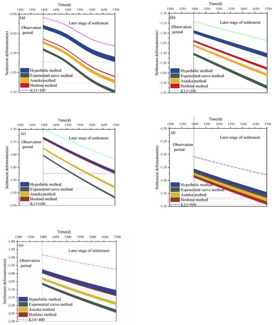
Figure 15. Empirical prediction model results’ distribution plot. (a) K13+100, (b) K13+200, (c) 13+600, (d) K13+900, (e) K14+400.

4. Discussion

4.1. Physical Mechanism of Permeability Influencing Prediction Accuracy

The simulation results (Figure 10 and Figure 12) revealed a strong positive correlation between the permeability coefficient ($K$) and the predictive performance of empirical models. Specifically, as $K$ increased, both systematic error and random error decreased following a power function trend. This phenomenon can be attributed to the consolidation mechanism of soft soil.

According to Terzaghi’s one-dimensional consolidation theory, higher permeability accelerates the dissipation of excess pore water pressure [23]. In high-permeability foundations, the settlement curve enters the secondary consolidation phase or stabilization phase earlier within the same observation window. Consequently, the non-stationary characteristics of the time series diminish, and the data trend becomes more deterministic and asymptotic. This reduces the complexity of curve fitting, thereby enhancing both accuracy and stability. Conversely, for low-permeability soils ($K<2.76\times {10}^{-4}$ m/d), the consolidation process is prolonged, and the observational data remain in a highly nonlinear and non-stationary development stage for a longer duration. This makes empirical models highly sensitive to random noise, a challenge also noted by Huang et al. [43] in their study on marine clay settlement.

4.2. Performance Trade-Off and Mathematical Characteristics of Models

A critical finding of this study is the distinct performance differentiation among the four models, which relates to their mathematical definitions:

Hyperbolic Method (Highest Accuracy, Lower Stability): Our results rank the Hyperbolic method as the most accurate (Systematic Error $\approx 3.2\%$). This aligns with the consensus in the literature that the Hyperbolic method best describes the stress–strain relationship of nonlinearity in soils [42]. However, its stability was the poorest (Random Error $>6$ mm). Mathematically, the Hyperbolic formulation ($S_t=t/(\alpha +\beta t)$) relies heavily on the slope parameter $\beta$ to determine final settlement. Early-stage data fluctuations can cause significant variance in $\beta$ estimation, leading to unstable predictions. This sensitivity confirms the observations by Tan et al. [16], who suggested that the Hyperbolic method is less reliable when data are sparse or noisy.

Hoshino Method (Highest Stability): The Hoshino method demonstrated superior stability (Random Error $\approx 3.8$ mm). This is likely because the Hoshino model relates settlement to the square root of time ($\sqrt{t}$). The square root function inherently acts as a “smoothing filter” for high-frequency random noise in field observations, making the model more robust against outliers compared to the Hyperbolic or Exponential models.

Asaoka and Exponential Methods: The Asaoka method showed limited applicability in low-permeability scenarios. This is consistent with the findings of Magnan [25], who noted that the Asaoka method requires equidistant data and a clear linear recurrence relationship, which is difficult to establish in the chaotic early stages of slow-consolidating soil.

4.3. Effectiveness of the Entropy-Based Evaluation Framework

Traditional model selection often relies solely on the correlation coefficient ($R^2$) or Root Mean Square Error (RMSE) [39]. However, our study demonstrates that a high $R^2$ does not necessarily guarantee a robust prediction of final settlement. For instance, the Hyperbolic method maintained $R^2\ge 0.98$ even when its random error was high.

By introducing the Entropy Weight Method (EWM), this study constructed a comprehensive index integrating goodness-of-fit, accuracy, and stability. The field validation (Table 2) confirmed the simulation-derived ranking: Hyperbolic > Hoshino > Exponential > Asaoka. Notably, in section K14+400, where data noise was presumably higher (indicated by larger random errors), the Hoshino method achieved a better comprehensive index (0.70) than the Hyperbolic method (0.52). This validates that the proposed multi-metric framework is more rigorous for complex engineering environments than single-metric evaluations.

4.4. Practical Implications for HSR Maintenance

Based on the comprehensive ranking and geological sensitivity analysis, the following strategies are proposed for high-speed railway (HSR) settlement monitoring:

Model Selection Strategy: For sections with high permeability or treated foundations (e.g., PVD-improved ground), the Hyperbolic Method is recommended for its high precision. For sections with low permeability or significant observational noise, the Hoshino Method should be prioritized to ensure conservative and stable predictions.

Data Quality Control: Since prediction accuracy is highly dependent on permeability ($K$), engineering measures that accelerate drainage (e.g., surcharge preloading) can fundamentally improve the quality of deformation monitoring data.

Monitoring Frequency: For low-permeability zones, the observation frequency should be increased to compensate for the “non-stationary” nature of the data, thereby reducing the random error component identified in this study.

5. Conclusions

This study addresses the complexity of predicting settlement in high-speed railway soft foundations by establishing a Monte Carlo-based simulation framework and an entropy-based evaluation system. The key findings are as follows:

Stochastic Simulation Framework: A novel data processing method was developed to quantitatively simulate “non-equidistant, time-varying, and random noise” characteristics in observational data. Validated against theoretical benchmarks (relative error < 1%), this framework successfully generated large-scale datasets that replicate realistic engineering conditions, providing a robust foundation for model stress-testing.

Model Performance Trade-offs: The Hyperbolic Method demonstrated the highest accuracy (Systematic Error: 3.2% ± 1.1%) and goodness-of-fit ($R$: 0.983 ± 0.006) but exhibited sensitivity to noise. Conversely, the Hoshino Method offered optimal stability (Random Error: 3.8 ± 2.0 mm), making it robust against data fluctuations. A strong positive correlation ($R^2>0.92$) was identified between the soil permeability coefficient and prediction performance, indicating that faster drainage significantly enhances prediction reliability.

Comprehensive Ranking: An evaluation framework based on the Entropy Weight Method (EWM) was constructed, assigning objective weights to stability (40.3%), goodness-of-fit (31%), and accuracy (28.7%). Validated by five engineering cases, the comprehensive performance ranking for natural soft foundations is: Hyperbolic > Hoshino > Exponential Curve > Asaoka.

Future Directions: While this study focused on natural soft foundations, future research should extend to complex ground treatments (e.g., pile-raft foundations) and explore the quantitative impact of observation frequency. Furthermore, integrating intelligent optimization algorithms (e.g., MOPSO, GA, LSTM, SVM) into this evaluation framework will be crucial for developing adaptive, real-time monitoring standards. Although the independent and identically distributed Gaussian noise assumption adopted in this study facilitates theoretical analysis, actual monitoring data may exhibit more complex statistical characteristics. Future research will consider noise models that better align with engineering reality.

References

- TB 10001-2016; Code for Design of Railway Earth Structure. China Railway Publishing House: Beijing, China, 2017.
- Li, T.F. Mapping relationship and control standard of post-construction settlement deformation of subgrade and ground of 400 km/h high speed railway. Railw. Eng. 2023, 63, 107–112. [Google Scholar] [CrossRef]
- Skempton, A.W.; Bjerrum, L. A contribution to the settlement analysis of foundations on clay. Géotechnique 1957, 7, 168–178. [Google Scholar] [CrossRef]
- Xia, J.; Huang, G.-L.; Yan, S.-B. Behaviour and engineering implications of recent floodplain soft soil along lower reaches of the Yangtze River in Western Nanjing, China. Eng. Geol. 2006, 87, 48–59. [Google Scholar] [CrossRef]
- Lin, D.-F.; Lin, K.-L.; Hung, M.-J.; Luo, H.-L. Sludge ash/hydrated lime on the geotechnical properties of soft soil. J. Hazard. Mater. 2007, 145, 58–64. [Google Scholar] [CrossRef]
- Tang, Y.Q.; Ren, X.; Chen, B.; Song, S.; Wang, J.X.; Yang, P. Study on land subsidence under different plot ratios through centrifuge model test in soft-soil territory. Environ. Earth Sci. 2012, 66, 1809–1816. [Google Scholar] [CrossRef]
- Mesri, G.; Choi, Y.K. Settlement analysis of embankments on soft clays. J. Geotech. Eng. 1985, 111, 441–464. [Google Scholar] [CrossRef]
- TJ [2006] No. 158; Technical Guide for Assessment of Ballastless Track Laying Conditions on Passenger Dedicated Lines. China Railway Publishing House: Beijing, China, 2006.
- Q/CR 9230-2016; Observation and Evaluation Specification for Settlement Deformation of Railway Engineering. China Railway Publishing House: Beijing, China, 2017.
- Cheng, C.; Sa-Ngasoongsong, A.; Beyca, O.; Le, T.; Yang, H.; Kong, Z.; Bukkapatnam, S.T.S. Time series forecasting for nonlinear and non-stationary processes: A review and comparative study. IIE Trans. 2015, 47, 1053–1071. [Google Scholar] [CrossRef]
- Liu, Y.; Wu, H.; Wang, J.; Long, M. Non-stationary transformers: Exploring the stationarity in time series forecasting. In Proceedings of the 36th International Conference on Neural Information Processing Systems, New Orleans, LA, USA, 28 November–9 December 2022; Curran Associates Inc.: Red Hook, NY, USA, 2022; pp. 9881–9893. Available online: https://dl.acm.org/doi/10.5555/3600270.3600988 (accessed on 29 January 2026).
- Juang, C.H.; Wang, L. Reliability-based robust geotechnical design of spread foundations using multi-objective genetic algorithm. Comput. Geotech. 2013, 48, 96–106. [Google Scholar] [CrossRef]
- Li, L.W.; Wu, Y.P.; Miao, F.S. Prediction of non-equidistant landslide displacement time series based on grey wolf support vector machine. J. Zhejiang Univ. Sci. 2018, 52, 1998–2006. [Google Scholar] [CrossRef]
- Wang, L.; Li, T.; Wang, P.; Liu, Z.; Zhang, Q. BiLSTM for predicting post-construction subsoil settlement under embankment: Advancing sustainable infrastructure. Sustainability 2023, 15, 14708. [Google Scholar] [CrossRef]
- Raubitzek, S.; Neubauer, T. A fractal interpolation approach to improve neural network predictions for difficult time series data. Expert Syst. Appl. 2021, 169, 114474. [Google Scholar] [CrossRef]
- Tan, Q.; Wei, J.; Hu, J. Applications of wavelet neural network model to building settlement prediction: A case study. Sens. Transducers 2014, 169, 1–8. [Google Scholar]
- Yu, Y.T.; Zheng, J.G.; Zhang, J.W.; Huang, X.; Xu, W.T. Prediction of settlement based on fusion model of Kalman filter and exponential smoothing algorithm. Chin. J. Geotech. Eng. 2021, 43, 127–131. [Google Scholar] [CrossRef]
- Zhou, J.; Ma, J.L.; Xu, H.; Huang, X.F. Application of EMD denoising method in subgrade settlement prediction of high-speed railways. J. Vib. Shock 2016, 35, 66–72. [Google Scholar] [CrossRef]
- Zhang, P.; Wu, H.-N.; Chen, R.-P.; Chan, T.H.T. Hybrid meta-heuristic and machine learning algorithms for tunneling-induced settlement prediction: A comparative study. Tunn. Undergr. Space Technol. 2020, 99, 103383. [Google Scholar] [CrossRef]
- Yen, N.Y.; Chang, J.-W.; Liao, J.-Y.; Yong, Y.-M. Analysis of interpolation algorithms for the missing values in IoT time series: A case of air quality in Taiwan. J. Supercomput. 2020, 76, 6475–6500. [Google Scholar] [CrossRef]
- Chen, W.H.; Luo, Q.; Wang, T.F.; Jiang, L.W.; Zhang, L. Bi-LSTM based rolling forecast of subgrade post-construction settlement with unevenly spaced time series. J. Zhejiang Univ. Sci. 2022, 56, 683–691. [Google Scholar] [CrossRef]
- Kliesch, K.; Johmann, S.; El-Mossallamy, Y.; Neidhart, T. Zur Setzungsprognose bei Erdbauwerken mit fester Fahrbahn—Erfahrungen an 43 km Neubaustrecke. In Proceedings of the Entwicklungen Bodenmechanik Bodendynamik Geotechnik; Springer: Mainz, Germany, 2002; pp. 333–346. [Google Scholar]
- Liu, J.F.; Zhao, G.T. Selection of prediction model used in assessment of railway subgrade subsidence. Railw. Eng. 2010, 50, 64–68. [Google Scholar] [CrossRef]
- Ying, H.W.; Huang, Z.J.; Ge, H.B.; Shen, H.W.; Wang, K.H.; Gong, X.N. Curve-fitting method for settlement based on staged loading condition and its engineering application. J. Southeast Univ. Sci. Ed. 2021, 51, 300–305. [Google Scholar] [CrossRef]
- Wang, X.Y. Research of Prediction Method for Subgrade Settlement on Railway Passenger Dedicated Line. Master’s Thesis, Institute of Rock and Soil Mechanics, Chinese Academy of Sciences, Wuhan, China, 2009. Available online: https://d.wanfangdata.com.cn/thesis/Y1612023 (accessed on 29 January 2026).
- Leng, W.M.; Yang, Q.; Nie, R.S.; Yue, J. Study of post-construction settlement combination forecast method of high-speed railway bridge pile foundation. Rock Soil Mech. 2011, 32, 3341–3348. [Google Scholar] [CrossRef]
- Qin, P.; Cheng, C.; Su, H. A GA-FGM-RTA combined model for predicting seawall settlement in under insufficient data volume. Soft Comput. 2025, 29, 1133–1146. [Google Scholar] [CrossRef]
- Mustafa, R.; Kumar, K.; Shankar, R. Appraisal of numerous machine learning techniques for the prediction of consolidation settlement subjected to placing of the fill. Transp. Infrastruct. Geotechnol. 2025, 12, 120. [Google Scholar] [CrossRef]
- Liu, Z.; Wang, L.; Li, T.; Guo, H.; Chen, F.; Zhao, Y.; Zhang, Q.; Wang, T. A Monte Carlo simulation framework for evaluating the robustness and applicability of settlement prediction models in high-speed railway soft foundations. Symmetry 2025, 17, 1113. [Google Scholar] [CrossRef]
- Sridharan, A.; Murthy, N.S.; Prakash, K. Rectangular hyperbola method of consolidation analysis. Géotechnique 1987, 37, 355–368. [Google Scholar] [CrossRef]
- Zeng, G.X.; Yang, X.L. Analysis of sand well foundation subsidence. J. Zhejiang Univ. Eng. Sci. 1959, 3, 34–72. Available online: https://kns.cnki.net/KCMS/detail/detail.aspx?dbcode=CJFQ&dbname=CJFD7984&filename=ZDZC195903001 (accessed on 29 January 2026).
- Asaoka, A. Observational procedure of settlement prediction. Soils Found. 1978, 18, 87–101. [Google Scholar] [CrossRef]
- Kong, J.; Kim, H.; Chun, B. Settlement analysis for improvement effect of soft ground method in Incheon Cheongna site. J. Korean GEO-Environ. Soc. 2012, 13, 19–26. Available online: https://www.koreascience.kr/article/JAKO201219066229964.pub?&lang=en (accessed on 29 January 2026).
- Park, E.; An, D.; Chae, H.; Chun, B. A study on the applicability of prediction methods for long-term ground settlement in soft ground of Gyeongnam area. J. Korean GEO-Environ. Soc. 2012, 13, 5–13. Available online: https://koreascience.kr/article/JAKO201219066192921.page (accessed on 29 January 2026).
- Björck, Å. Least squares methods. In Handbook of Numerical Analysis; Elsevier: Amsterdam, The Netherlands, 1990; Volume 1, pp. 465–652. ISBN 978-0-444-70366-8. [Google Scholar]
- Du, M.F.; Li, J.H.; Zheng, X.Y.; Lu, L.L. Variation law of excess pore pressure of soft foundation under multi-stage linear loading. China Sci. 2022, 17, 851–856. [Google Scholar] [CrossRef]
- TB 10038-2022; Specification for Special Rock and Soil Investigation of Railway Engineering. China Railway Publishing House: Beijing, China, 2022.
- Li, Q.F.; Wang, Z.; Yu, Y. Optimization of area replacement ratio of stone column based on robustness principle. J. Jilin Univ. Sci. Ed. 2022, 52, 171–180. [Google Scholar] [CrossRef]
- Zhu, Y.; Tian, D.; Yan, F. Effectiveness of entropy weight method in decision-making. Math. Probl. Eng. 2020, 2020, 3564835. [Google Scholar] [CrossRef]
- Wu, R.M.X.; Zhang, Z.; Yan, W.; Fan, J.; Gou, J.; Liu, B.; Gide, E.; Soar, J.; Shen, B.; Fazal-e-Hasan, S.; et al. A comparative analysis of the principal component analysis and entropy weight methods to establish the indexing measurement. PLoS ONE 2022, 17, e0262261. [Google Scholar] [CrossRef]
- Yang, Y. Elements of information theory. J. Am. Stat. Assoc. 2008, 103, 429. [Google Scholar] [CrossRef]
- Zhao, J.Z. Research on settlement of soft clay ground in Lianyungang. Chin. J. Geotech. Eng. 2000, 22, 643–649. [Google Scholar] [CrossRef]
- Huang, W.X. Engineering Properties of Soils; China Water & Power Press: Beijing, China, 1983; pp. 138–139. [Google Scholar]
Disclaimer/Publisher’s Note: The statements, opinions and data contained in all publications are solely those of the individual author(s) and contributor(s) and not of MDPI and/or the editor(s). MDPI and/or the editor(s) disclaim responsibility for any injury to people or property resulting from any ideas, methods, instructions or products referred to in the content. |
© 2026 by the authors. Licensee MDPI, Basel, Switzerland. This article is an open access article distributed under the terms and conditions of the Creative Commons Attribution (CC BY) license.