Abstract
This paper introduces a novel approach to anomaly-based failure forecasting that jointly optimizes both the ensemble function and the anomaly threshold used for decision making. Unlike conventional methods that apply fixed or classifier-defined thresholds, the proposed framework simultaneously tunes the threshold of the failure probability or anomaly score and the parameters of an ensemble function that integrates multiple machine learning models—specifically, Random Forest and Isolation Forest classifiers trained under diverse preprocessing configurations. The distinctive contribution of this work lies in introducing a weighted mean ensemble function, whose coefficients are co-optimized with the anomaly threshold using a global optimization algorithm, enabling adaptive, data-driven decision boundaries. The method is designed for predictive maintenance applications and validated using sensor data from three industrial domains: aluminum anode production, plastic injection molding, and automotive manufacturing. The experimental results demonstrate that the proposed combined optimization significantly enhances forecasting reliability, improving the Matthews Correlation Coefficient by up to 6.5 percentage units compared to previous approaches. Beyond its empirical gains, this work establishes a scalable and computationally efficient framework for integrating threshold and ensemble optimization in real-world, cross-industry predictive maintenance systems.
1. Introduction
This paper pertains to an algorithm which employs machine learning methods to forecast industrial equipment stoppages in various domains. This capability is critical, as early warnings for potential failures allow plant personnel to take proactive maintenance measures. Based on input from process experts, the ideal forecasting horizon for such alerts is 30 min–2 h before a failure occurs. Particularly, the work builds on our earlier research [1,2,3,4] by investigating the application of supervised and unsupervised machine learning techniques for anomaly detection, with the goal of forecasting failures in the context of condition-based predictive maintenance [5,6]. Our most recent conference paper [2] extended the older work in two directions. The first was the ensemble of multiple classifiers for a common prediction. The second and most important was the integration of an optimization method for the threshold of the failure probability or anomaly score predicted by the classifier above which the classifier raises an alert. This threshold was previously determined by the single classifier itself, without always yielding optimal results in that way. That work was further extended here by the following:
- Introducing a new family of candidate ensemble functions to further improve performance, namely the weighted mean, where the weights are automatically optimized parallel to the failure probability or anomaly score threshold;
- Extending the experimental results from the aluminum also to the plastic and automotive domains;
- Enhancing the literature report regarding both anomaly threshold optimization and ensemble methods.
The remainder of this paper is organized as follows. Section 2 includes the study of the bibliography. Section 3 recaps the industrial data set description, Section 4 presents the methodology, Section 5 presents the experimental results, and Section 6 discusses them more profoundly and concludes the work.
2. Related Work
Numerous studies have investigated the optimization of anomaly score thresholds in binary classification settings. Among the most relevant and recent contributions is the work in [7], where the authors optimized the classifier’s probability threshold to enhance performance across various metrics, such as precision, the Matthews Correlation Coefficient (MCC), the F-measure, and the geometric mean of the true positive and true negative rates. Their approach achieved notably better results than with the default threshold. In [8], a robust algorithm based on Isolation Forest (IF) [9] was introduced and evaluated using performance indicators like the Area Under the Receiver Operating Characteristic (AUC-ROC) curve and the Area Under the Precision–Recall Curve (AUPRC). Comparable efforts can be found in [10,11,12]. The study in [13] highlights a limitation of ROC and precision–recall curves, noting that they do not inherently suggest an optimal threshold, and that relying on them in the context of imbalanced data may lead to misleading interpretations. To address this, the authors proposed a new metric, MCC-, aimed at improving threshold selection via confusion matrix optimization. However, both their findings and our own experiments indicate that the MCC and F-measure often reach their peaks simultaneously. As a result, this new metric has not shown significant added benefit, at least within the context of our implementation. In [14], the authors provided new insight into maximizing scores in the contexts of binary and multi-label classification. In parallel, ref. [15] demonstrated the effectiveness of Long Short-Term Memory (LSTM) networks for anomaly detection in spacecraft telemetry data, augmenting the model with an unsupervised, non-parametric anomaly thresholding approach. The research in [16] explores complex performance measures in binary classification by identifying two key properties: a so-called Karmic property and a more technical threshold quasi-concavity property. These properties ensure that the Bayes optimal classifier is a threshold function of the conditional probability of the positive class. The study in [17] introduces a method that dynamically applies a trustworthy approximated partial AUC-ROC loss while the optimal threshold is selected to avoid false negatives. The optimization of the anomaly thresholds of a Support Vector Machine (SVM) for anomaly detection, by introducing a quantitative measure, has also been proposed in [18], whereas ref. [19] proposed a deep-learning-based anomaly detection model for Internet of Things (IoT) networks incorporating adaptive thresholding techniques. Similarly, in [20], a comprehensive analysis of the IF algorithm enhanced with adaptive thresholding mechanisms has been proposed with improved performance. In [20], an in-depth study and improvement of the IF have also been examined to detect anomalies in industrial applications by comparing various approaches. Also, ref. [21] introduced an automatic method for optimizing the class probability threshold in a Convolutional Neural Network Transformer (CNN-Transformer) model, using numerical gradient-based optimization techniques. Lastly, ref. [22] addresses model architecture optimization and thresholding.
Ensemble learning was originally introduced by Zhou (see updated edition in [23]), demonstrating that combining multiple base models can help to mitigate the errors of individual models. More recently, ref. [24] proposed an Ensemble Learning-Based Detection framework that integrates a selection of established detection methods, including traditional linear ensemble techniques such as the maximum, average, and weighted average, as well as a novel deep ensemble method. This study also introduced a new metric designed to evaluate detection accuracy, robustness, and the capability for multi-step prediction. A comparable strategy was previously adopted in [25]. In [26], the authors applied an optimization strategy using swarm intelligence in conjunction with ensemble learning to address the feature selection problem, yielding promising results. Similarly, ref. [27] presented a software architecture that combines ensemble learning with high-performance computing to manage large-scale user activity data and enhance behavior classification. Meanwhile, ref. [28] proposed an ensemble method that integrates ten different machine learning algorithms, assigning weights to each through a k-fold cross-validation process. Another related study [29] introduced a stacked ensemble combining three supervised classifiers within a generalized linear modeling framework. In the domain of cybersecurity, ref. [30] explored network intrusion detection through two ensemble techniques, including a deep learning method (LSTM) that focused on computing weights or linear combinations across base models. Additionally, ref. [31] addressed the issue of data labeling within semi-supervised learning contexts. SMOTEBoost [32] is a novel ensemble approach capable of learning from imbalanced datasets based on a combination of the Synthetic Minority Over-sampling TEchnique (SMOTE) algorithm and the boosting procedure, with improved performance in the minority class and overall improved F-values. A survey of multiple classifier systems was examined from the point of view of Hybrid Intelligent Systems, such as diversity and decision fusion methods, in [33]. A relevance-weighted ensemble model for anomaly detection in switching data streams was proposed in [34], learning from the history of normal behavior in data streams while accounting for the fact that not all time periods in the past are equally relevant. Similarly, another ensemble method for anomaly detection and distributed intrusion detection in mobile Ad-hoc networks was proposed in [35], using a three-level hierarchical system for data collection, processing, and transmission. The overall results also confirmed the benefits of averaging in detection accuracy. Furthermore, HELAD [36], a novel network anomaly detection model based on heterogeneous ensemble learning based on the organic integration of multiple deep learning techniques such as the Damped Incremental Statistics algorithm, Autoencoder, and LSTM, provided better adaptability and accuracy than other state-of-the-art algorithms. Unsupervised ensemble learning, also known as consensus clustering, focuses on determining the most effective way to merge results from multiple clustering algorithms. In this area, ref. [37] proposed a weighting strategy that leverages internal clustering quality metrics. More recently, ref. [38] introduced a sampling method to enhance financial distress prediction, developing and evaluating multiple ensemble models designed to address class imbalance in financial datasets. In our study, it was found that using standard ensemble functions was adequate for our purposes.
While prior research has made significant contributions to threshold optimization and ensemble learning, existing methods generally treat these two dimensions independently, rely on fixed or heuristically chosen ensemble schemes, or require repeated model retraining during optimization. In contrast, the present work bridges these gaps by introducing a unified, computationally efficient framework that simultaneously optimizes the anomaly score threshold and the ensemble function parameters—most notably the weighted mean coefficients—without refitting the underlying classifiers. This joint optimization not only leverages the strengths of threshold selection studies [7,13,14] and ensemble-based anomaly detection approaches [24,25,36], but also advances them by explicitly characterizing and exploiting the interaction between threshold choice and ensemble behavior. The resulting methodology improves the MCC, F-measure and accuracy across heterogeneous industrial domains. Unlike the dynamic or domain-specific thresholding schemes proposed in earlier works, the proposed approach provides a generalizable optimization strategy applicable to diverse forecasting horizons, ensemble functions, and model families, thereby overcoming the limitations related to fixed metrics, non-scalable optimization, or domain-restricted heuristics observed in the existing literature.
3. Dataset Description
Substantial raw data were available to analyze in the aluminum, plastic, and automotive domains, primarily because of the numerous timestamps. The data are categorized into two main types: input data, which consist of the analyzed signals used to detect anomalies for fault forecasting, and target data, which refer to reference stop data that the analysis attempts to correlate with the input data based on a specific forecasting horizon. Stops can be voluntary (triggered by plant operators, such as planned maintenance) or involuntary (referred to as faults/failures or breakdowns). The data analysis aims to identify the variables (or features) capable of predicting faults of the relevant type in a timely manner. Forecasting voluntary stops was excluded from the scope of this problem, as it is not always clear whether a voluntary action results from a recent anomaly. In cases of voluntary stops, it appears that the plant operators have already identified the potential problem. Further details for each domain are provided below.
3.1. Aluminum Domain
In our earlier study [4], the dataset covered a period of 2.5 years, with the time series data sampled every 2 to 5 s. In contrast, the present work narrows its focus to a 40-day interval, selected because it contains the majority of notable failure events (61 in total) and shows the strongest correlation between anomalies and the specific failures of interest. The sensor data capture various process variables from equipment in the “cold” chain of the anode production line, including the cooler, the paste mixer, and the preheating screw. Malfunctions in these components can negatively affect the quality of green anodes, such as by altering anode density. A detailed description of this production chain is available in our previous work, where it was identified that the cooler level is the most relevant variable for the early detection of anomalies, especially for cooler-related failures. Accordingly, the remainder of this paper will concentrate on that variable and failure type.
In addition to the process variables used for the classifier inputs, another dataset was also available, containing automatically logged equipment stoppages, including start and end times, and failure types, as recorded by an internal system. Since the study employs unsupervised learning, this dataset is used solely for evaluation purposes and not for training. Furthermore, process experts identified certain process signals, other than the cooler level, as indicators of potential failures when they drop below specific thresholds. These signals are referred to as “stop annotators”. A given time point is considered as corresponding to a failure if it is flagged as such either by the internal system or by a stop annotator. Typically, failures are detected first by stop annotators and slightly later by the internal logging system. If the internal system starts logging a failure within a failure period defined by a stop annotator, it is assumed that the failure (associated with the reason identified by the system) actually begins at the initial abnormal timestamp identified by the annotator. Conversely, failure intervals recorded only by annotators (and not confirmed by the internal system) are treated as undefined in terms of failure type. These relationships and assumptions are illustrated in Figure 1.
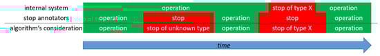
Figure 1.
Algorithm’s consideration for stop periods and their types based on information by the internal system and the stop annotators in the aluminum domain. Reproduced with permission from [2,3,4].
3.2. Plastic Domain
In the previous work [4], data from five injection molding machines for capsule and lid production with various types of failures increasing the product rejection rate were analyzed within a period of about 1 year, with a timestamp step of 6–10 s. The process variables are related to the cycle time and the time needed for its different phases, temperatures, cushion, etc. This work focuses only on one of the machines (no. 49), which proved to involve the most interesting anomaly (related to the mold open time process variable) correlated with 123 relevant upcoming failure instances (associated with a plastic part stuck in a core or cavity).
In this domain, there is no internal system that automatically registers the stops, so the operators register them manually along with their reason. The existence of a stop may also be inferred by the lack of process cycles (which does not indicate the reason, though), which is being identified while the cycle counter variable remains constant for at least double the normal cycle time. Similarly to aluminum, it was assumed that a timestamp belongs to a stop interval if it is recorded by either of the two methods mentioned earlier. In the plastic domain, it was also assumed that a stoppage continues for the first 5 min after the cycle counter begins to increase. This is because both process experts and our own visual observations indicate that during the initial cycles after a stop, the process and the related data have not yet stabilized, so the model may interpret such behavior as anomalous. The definition of stop periods in the plastic domain is shown in Figure 2.
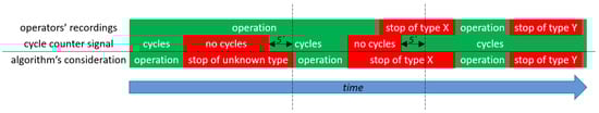
Figure 2.
Algorithm’s consideration for stop periods and their types based on information by the operators’ recordings and the cycle counter signal in the plastic domain. It was assumed that a stop continues at least for the first 5 min after cycles restart. Reproduced with permission from [4].
3.3. Automotive Domain
The dataset’s time interval corresponds to the period when most sensors were available and lasts about 4.5 months. Each sensorial variable has its own timestamps, with variable sampling steps, but generally are close to 1 min. These variables correspond to the phosphate and electrocoat booths use case, involving various problems known by the process experts. After a preliminary analysis of the data, it turned out that, only for the problem of crystallization in the fifth booth (because the water temperature entering the fifth booth after the valve exceeds a predefined threshold), the application of the algorithm makes sense, because the threshold was exceeded several times and it seems that this can be forecasted a couple of hours before. Thus, in the automotive domain, the remainder of this paper will focus only on this problem. To avoid crystallization in the chemical material loop, the automatic valve is put in the half-open position. However, it is even more beneficial to forecast the exceedance of the temperature threshold after the valve.
In this domain, the stop intervals were defined as those when the temperature exceeded the upper threshold, which is not mentioned in the paper due to confidentiality.
4. Materials and Methods
The methodological flow involves firstly preprocessing (aggregaton, feature computation, and variable selection), then base classification models fitting, and, finally, ensemble function and anomaly threshold optimization to define the ensemble model.
4.1. Training Details
The chosen unsupervised classifier for this study was Isolation Forest (IF), whereas the supervised one was Random Forest (RF). These are fast, well-performing, and memory-efficient architectures, which are suitable for big data and do not require them to be scaled, so they were preferred over other alternatives, like Multi-Layer Perceptrons, Support Vector Classifiers [39], Elliptic Envelope [40] and Local Outlier Factor [41]. That is, IF and RF were selected due to their favorable theoretical properties for large-scale failure forecasting. More specifically, both methods scale linearly (up to logarithmic factors) with data size, are invariant to feature scaling, and make minimal distributional assumptions. IF identifies anomalies via random partitioning rather than density estimation, making it robust to high-dimensional, non-Gaussian sensor data. RF leverages ensemble averaging to reduce variance and handle severe class imbalance, while remaining computationally tractable and interpretable. In contrast, kernel-based methods, density estimators, and deep learning architectures require stronger assumptions, extensive tuning, or large labeled datasets, which are often unavailable in industrial failure settings. The classifiers were implemented using the Python (3.13.5) library scikit-learn (scikit-learn, http://scikit-learn.org/stable/, accessed on 23 December 2025). Generally, unsupervised learning was preferred in our work for two main reasons. First, unsupervised methods avoid the need to define a fixed forecasting horizon for labeling data; this is only needed for performance evaluation. Second, unsupervised learning eliminates the requirement to divide the dataset into training and test sets. Supervised learning was also used only in the automotive domain, since IF standalone proved to be inadequate to fully recognize the anomalous pattern that should be correlated with upcoming failures, but, instead, prioritizes anomalies irrelevant to failures, viewing them as more important.
Among the IF hyperparameters, the number of estimators is the most influential, as increasing it generally improves performance, albeit at the expense of greater computational time and memory usage. A value of 20 estimators was chosen, as higher values yielded no noticeable performance gains. Notably, the contamination parameter, which defines the proportion of data points considered outliers, has little relevance in this work. This is because the proposed method triggers alerts based on an optimized anomaly score threshold, independent of the contamination setting. Finally, the random state was set to zero for reproducibility, since it affects the results only slightly. For the other hyperparameters, the default values mentioned in the library documentation were considered (automatic number of samples and input features to train each base estimator, no bootstrap, no warm start etc.).
Regarding the modified hyperparameters of RF, the number of estimators was set to ten to avoid excessive computational burden, and this number proved to be sufficient. Both Gini and entropy criteria to measure split quality were tested, but in the end models based on Gini were preferred due to slightly better results. The maximum depth of 20 appeared to correspond to the near–best trade-off between underfitting and overfitting. The classes weights were selected to be balanced due to the severe imbalance of the classes, since in the automotive domain only 1.74% of the timestamps during operation (that is, not corresponding to a stop) are at a distance from an upcoming failure less than 2 h, which is the considered forecasting horizon based on the needs of the industry. Finally, the random state was set to zero, in accordance with the logic used with respect to IF. For the other hyperparameters, the default settings mentioned in the library documentation were considered (minimum number of samples required to split an internal node = two, minimum samples required to be at a leaf node = one, minimum weighted fraction of the sum total of input samples weights required to be at a leaf node = zero, number of features to consider when looking for the best split = square root of all features, unlimited leaf nodes for tree growing in best–first fashion, node split whenever impurity does not worsen, bootstrap, no out-of-bag samples, no warm start, no pruning, all samples used for each base estimator training, no monotonicity constraints etc.).
4.2. Evaluation Metrics
When unsupervised learning is used, the same dataset (all data) served both for training and evaluation, whereas in supervised learning the earliest 70% of the timestamps were used as the training set and the remaining 30% as the test set. As discussed in our previous work [3,4], standard evaluation metrics, such as precision, recall, F-measure, and accuracy, are derived from the confusion matrix. However, for binary classification tasks, particularly with imbalanced data (as is the case here), the aforementioned MCC stands out as a more objective metric. Thus, it was used as the primary criterion for comparing models during both forward feature selection and anomaly score threshold optimization. This work’s evaluation emphasizes the added value brought by the proposed methodological enhancements. Typically, the model that achieves the best MCC also performs best in terms of the F-measure and accuracy. MCC is preferred because its baseline (neutral) value is always zero, regardless of class distribution, making it less sensitive to imbalance. In contrast, precision and recall offer a more limited view, as each considers only part of the confusion matrix and may not fully reflect the overall performance of the classifier.
4.3. Data Preprocessing Details
Preprocessing followed the same approach as in our earlier work [4], and is therefore only briefly summarized here.
4.3.1. Problem Formulation
Our task is framed as a binary classification problem. Only time points during normal operation (that is, when no stoppage of any kind occurs) are analyzed. Each of these time points is assigned a binary label: it is marked as abnormal (negative class) if a relevant failure is expected to occur within a predefined forecasting horizon, and as normal (positive class) otherwise. In the aluminum domain, relevant failures include those logged by the internal system as cooler related, as well as unregistered failures, which exhibit similar cooler level anomalies within the analysis window. In the plastic domain, the two targeted failure types are those involving plastic parts becoming stuck in either the core or the cavity, as previously discussed. And, finally, in the automotive domain, the relevant failure is associated with the aforementioned exceedance of the temperature threshold of crystallization.
4.3.2. Aggregation
To ensure a consistent time step for classification, the data were aggregated using a 10 s interval for the aluminum domain, a 1 s interval for the plastic domain and a 1 min interval for the automotive domain. The sampling step per domain is selected so that it is close to the average sampling step of the raw data. All these choices are efficient in terms of memory usage. In cases where data were missing, linear interpolation was applied, as long as the gap between the consecutive timestamps did not exceed 1 min in the aluminum and plastic domains, and 2 min in the automotive domain.
4.3.3. Feature Computation
At each time point, features can be extracted from a rolling window containing the most recent data. These optional features can be used for the input to the classifier and include the mean, standard deviation, maximum, minimum, and trend (estimated as proportional to the slope from linear regression on the raw variable within the window), as well as frequency, which was calculated using the power spectrum via the periodogram from the scipy Python library (scipy, https://docs.scipy.org, accessed on 23 December 2025). The use of a raw time series value is also optional. In some models presented in this study, both feature extraction and time lagging were applied to the original time series. The user selects the candidate features and time lags based on insight from the visual observation of the raw data to reduce computational time; however, automatic variable selection follows afterwards, as mentioned below.
4.3.4. Variable Selection over Time
The set of variables obtained through the earlier preprocessing steps can be restricted using the well-known, time-efficient forward feature selection policy, guided by the MCC yielded by training. This is a parameter-free method which selects step by step the best variable to add to the previously selected ones until MCC stops improving.
4.4. Anomaly Score Threshold Optimization and Ensemble Methods
In addition to making categorical predictions, supervised scikit-learn classifiers (like RF) also compute classes’ probabilities, whereas unsupervised ones (like IF) generate a continuous anomaly score that quantifies the degree of anomaly. In this study, the anomaly score is normalized using an affine transformation, mapping it to the range [0, 1], where 0 represents the most normal condition and 1 the most abnormal, and, as the score increases, the anomaly becomes more pronounced (as already happens with the probability for the abnormal class computed by supervised classifiers). If a prediction’s transformed anomaly score falls outside this range, it is clipped to the nearest bound.
The goal is to determine the optimal threshold for the failure probability (in case of RF) or normalized anomaly score (in case of IF), above which a prediction should be classified as a failure. To achieve this, MCC is used as the optimization criterion, aiming to maximize it. Therefore, the objective function is defined as the opposite of MCC, so that the Differential Evolution (DE) global minimization algorithm from scipy can be applied to find the optimal solution. DE was first introduced in [42] and has been shown in subsequent studies [43,44,45,46] to be the most stable and reliable optimization method. Additionally, as will be shown later, our comparative analysis between DE and other global optimizers supported by the library, namely basin-hopping [47], Dual Annealing [48], and Simplicial Homology Global Optimization (SHGO) [49], revealed that DE can find a better solution in a shorter time and with fewer function evaluations, which is expected since MCC entails expensive (since it is based on two time series vectors, each containing around – elements) black box evaluation and thus it cannot be analytically differentiated as well, and the decision variables are few. For the same reasons, DE was also preferred over hybrid Genetic Algorithm–Particle Swarm Optimization (GA-PSO) and multi-swarm PSO approaches, like Real-Coded Genetic Algorithm–Particle Swarm Optimization (RCGA-PSO) [50], Hybrid Multi-Swarm Particle Swarm Optimization (HMSPSO) [51,52], and the Matrix-Based Hybrid Genetic Algorithm (MBHGA) [53]. Unlike PSO- and GA-based hybrids, DE exploits difference vectors to generate self-adaptive search directions, resulting in fewer redundant evaluations. This behavior has been widely reported in the literature for problems with fewer than ten decision variables, as is the case in this work.
The methodology also supports combining multiple classification models to make a single prediction. In our recent conference paper [2], functions such as the mean, median, maximum, and minimum were applied to the normalized anomaly scores of individual models to compute the ensemble’s anomaly score. In this paper, this approach is extended by using a weighted mean ensemble function instead of the regular mean, with the weights optimized alongside the threshold. Since the last weight is determined by the others, it does not influence the decision variables, and a constraint is applied to ensure all the weights are non-negative and sum to one. Models within the same ensemble vary in some of their training arguments, but, for the sake of comparison and efficiency, they must share certain characteristics. These include the raw process variables, the failure types to be predicted, the data time range, the forecasting horizon, the sampling step (before and after preprocessing), the aggregation method (linear interpolation) and the threshold for handling missing values. A particular ensemble may include both supervised and unsupervised classifiers, since the failure probabilities and the normalized anomaly scores are considered comparable.
Mathematically, the optimization problem in the general case is
according to the following notation:
- : the ensemble function among the weighted mean with weights , median, maximum and minimum;
- : the anomaly threshold;
- : the anomaly score time series resulting from ensemble function ;
- : binary prediction time series resulting from anomaly score time series and anomaly threshold ;
- : binary ground truth time series indicating if an interesting failure is upcoming.
That is, the continuous decision variables are vector and scalar . Since the last weight depends on the previous ones, the problem dimension equals the number of base models. Apparently, when weight optimization is not considered, is just omitted in the above, so the only continuous decision variable is .
The parameters of the DE algorithm that were adjusted and influence its results are as follows:
- Bounds: Regarding the bounds of the decision variables, as mentioned before, the weighted mean coefficients must fall within the range from zero to one, and the same applies to the threshold because it refers to failure probability or normalized anomaly score.
- Tolerance: The relevant tolerance for convergence was set to zero (as was by default the case with the absolute tolerance), since the optimizer was found to stop too early for the required accuracy of the optimal solution.
- Maximum number of iterations: To avoid excessive optimization time, the maximum number of generations for evolving the entire population was limited to 400 (aluminum and plastic domains) or 1000 (automotive domain) when optimizing both the threshold and weights simultaneously, and 40 when only optimizing the threshold. During the experiments, the former limit was reached, whereas the latter was not reached sometimes, because the optimizer had already converged.
- Population size: The population size was kept small (five when optimizing both the threshold and weights simultaneously and ten when optimizing only the threshold) to minimize the number of function evaluations. Increasing the population size while decreasing the number of iterations proportionally (to maintain a similar total number of function evaluations) led to poorer results.
- Strategy: The differential evolution strategy was set to “rand2exp” to maximize the exploration; indeed, this choice proved to be crucial for the optimizer to find the global optimum, or, at least, a better solution.
The default values were used for the other parameters (mutation constant from 0.5 to 1 with dithering, recombination constant 0.7, random seed/generator not specified, polishing, Latin hypercube population initialization method, immediate updating, no initial guess to the minimization etc.), and additional details can be found in the library documentation.
The complete process of the anomaly score threshold optimization and ensemble methodology is illustrated in Figure 3 and rigorously described in Algorithm 1.
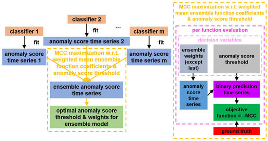
Figure 3.
Architecture of the anomaly threshold optimization and ensemble methods. Whatever applies to the anomaly score also applies to the failure probability.
| Algorithm 1 Weighted mean coefficients and anomaly threshold optimization algorithm |
| 1: . |
| 2: while no termination criterion applies (iteration number/population convergence) do |
| 3: do new MCC trial // population size × problem dimension function evaluations. |
| 4: . |
| 5: end while. |
| 6: polish solution // problem dimension + 1 function evaluations. |
| 7: get optimal MCC, optimal anomaly threshold and optimal weights except last. |
| 8: . |
5. Results
This section presents and analyzes the experimental results obtained by applying the described preprocessing, training, and evaluation methodology to the previously mentioned datasets from the aluminum, plastic, and automotive industries, highlighting the benefits of the extended methodology.
5.1. Aluminum Domain
5.1.1. Preliminary Observations
Within the 40-day period of analysis, there is a total operation interval of about 22 days. In total, 129 failure incidents immediately after normal periods were registered by any of the two aforementioned ways, including 61 interesting ones (11 were registered by the internal system as related to the cooler and 50 were undefined).
As discussed in our previous work [4], usually, before a breakdown of interest the cooler level starts to vibrate with increasing amplitude and a period of about 2 min. Based on the visual observation of this pattern just before each interesting failure instance, the values of the training arguments discussed in the following two subsections were determined.
5.1.2. Other Common Training Arguments
The values selected in our experiments for the arguments that must be common among models of the same ensemble have already been mentioned above. However, the following not necessarily common arguments, which are all related to the definition of the candidate variables for forward selection, happened to be also common in our implementation:
- Raw value inclusion in the candidate inputs: no.
- Mean/maximum/minimum computation: no.
- Standard deviation computation: yes.
5.1.3. Tuned Training Arguments
The optimal ensemble model was found for each combination of forecasting horizon (20 min/30 min/45 min) and ensemble function. The training arguments differing among the four base models of the same ensemble are summarized in Table 1.

Table 1.
Tuned training arguments among the individual models of the ensemble in the aluminum domain.
5.1.4. Forward Selection
Forward selection did not take place in the models of type a (according to Table 1), which had been studied in our previous work, because they involve a single input variable, i.e., the standard deviation of the cooler level. In the other cases, the following features were selected for each combination of arguments values ID and forecasting horizon:
- b—20 min: Standard deviation and frequency (2 min and 1 min) → three variables
- b—30 min/45 min: Standard deviation and frequency (1 min) → two variables
- c—20 min: Standard deviation (lags 0 and 50 s) and trend (lags 10 s and 70 s) → four variables
- c—30 min: Standard deviation (lags 0, 10 s, 30 s, 50 s, and 80 s) → five variables
- c—45 min: Standard deviation (lags 0, 20 s, 30 s, 50 s, and 70 s) → five variables
- d—20 min/30 min: Standard deviation (lags 0, 40 s, and 50 s) → three variables
- d—45 min: Standard deviation (lags 0, 30 s, 40 s, and 50 s) → four variables
5.1.5. Training Results
Table 2 shows the best classification results related to the confusion matrix, along with the improvement of MCC, as well as accuracy and the overall F-measure thanks to the threshold optimization and ensemble methods in the aluminum domain. For each considered forecasting horizon, the best value of each metric is underlined. The benefit of these methods is bigger for higher forecasting horizons, since they are at a higher distance from the average time difference between the start of failures of interest and the respective preceding anomalies (about 20 min). The positive impact of these methods is mostly related to the remarkable reduction in false negatives, although other values of the confusion matrix and some other metrics may worsen slightly. The usefulness of the ensembles is explained by the smoothing that they induce in the time series of anomaly score. Also, it appears that the optimal anomaly score threshold does not always correspond to a contamination equal to the actual percentage of abnormal timestamps, which was the assumption in our previous work in [4] (“None” case in the table). Among the model types of Table 1, type a is the less involved in the optimal ensembles. The median (which coincides with mean in cases of two base models) proves to be the most appropriate ensemble function in case of optimization without weights, although the min is usually better when threshold optimization does not take place either, to increase the percentage of alerts. However, the consideration of automatically optimized weights in the mean ensemble function renders it slightly better than any other function, at least in case of threshold optimization.
Table 2.
Best confusion-matrix-related evaluation metrics showing the benefit from anomaly score threshold and ensemble weights optimization in the aluminum domain. T = threshold optimization, wE = ensemble with weighted mean ensemble function and weight optimization, E = ensemble with selection of function among the mean, median, maximum, and minimum, EFW = ensemble function or weights of the weighted mean, AID = arguments IDs, TP = True Positives, FN = False Negatives, FP = False Positives, TN = True Negatives, Pn%/Rn%/Fn% = precision/recall/F-measure of normal class (%), Pa%/Ra%/Fa% = precision/recall/F-measure of abnormal class (%), Pm%/Rm%/Fm% = mean precision/recall/F-measure from classes (%), Fh% = harmonic mean of Pm% and Rm%, Acc% = accuracy (%), and nfev = number of objective function (MCC) evaluations. Underlined values are the best for the respective rows and forecasting horizons.
Figure 4 shows a representative (for most cooler incidents and incidents identified only by stop annotators in the analyzed period) example of the behavior of the cooler level during the latest operation time before a failure of interest identified only by the stop annotators (right endpoint of plot’s time interval) begins on 20 January 2018. It illustrates the remarkable reduction in false negatives achieved through anomaly score threshold optimization and ensemble methods for a 45 min forecasting horizon, as shown in Table 2. Each of the best individual models without optimization raises false alarms at different timestamps before the gradual anomalous vibration related to the upcoming failure begins, but the ensemble method with the optimization of the weighted mean coefficients and anomaly score threshold raises alerts only after the vibration has started. Such false alarms appear even for higher distances from the upcoming failures than those shown in the figure, so the slight reduction in true negatives is less important. More generally, the fewer false alarms compared to the initial method are obvious from Figure 5.
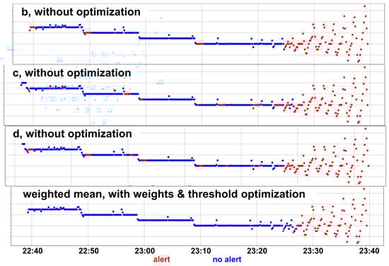
Figure 4.
Representative example of the behavior of the most critical raw variable for forecasting in the aluminum domain during the latest operation time before a failure of interest. The colors correspond to the binary predictions of the best models with 45 min forecasting horizon.
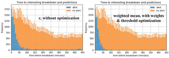
Figure 5.
Stacked histograms of failure alert presence/absence as a function of time before breakdown in the aluminum domain, for cooler stops and stops identified only by the stop annotators, for the best models with 45 min forecasting horizon.
5.2. Plastic Domain
5.2.1. Preliminary Observations
Within the 1-year period of analysis, the clear duration with operation and available data is about 5 months. Among the 1212 stops that occurred in machine 49 during this period, 567 correspond to failures (and the rest to voluntary stops, like maintenance), 229 of which are interesting (i.e., attributed to plastic part stuck in core or cavity). However, data within a 75 h period (ten times the forecasting horizon of 7.5 h eventually considered in our previous work [4] and also here) before the failure and after the previous stop exist in only 142 interesting cases (30 related to plastic part stuck in core and 112 to plastic part stuck in cavity).
5.2.2. Other Common Training Arguments
Based on the visual observation of the data and preliminary training trials, the following not necessarily common arguments happened to also be common in our implementation:
- Raw value inclusion in the candidate inputs: yes.
- Mean/minimum computation: yes.
- Standard deviation/trend/frequency computation: no.
- Feature window size: 30 min.
- Maximum lagging steps: 0.
5.2.3. Tuned Training Arguments
In this domain, the only tuned training argument was the one related to maximum computation. Just in case it is not computed, two values were considered for the random state hyperparameter of the classifier, since it proved to remarkably affect performance. Hereafter, these base models will be denoted as follows:
- a0/a1: Model without maximum computation and random state 0/1, respectively;
- b: Model with maximum computation.
5.2.4. Forward Selection
The following features were selected for each arguments values ID:
- a0: mean and minimum → two variables
- a1: minimum → one variable
- b: raw value, mean, maximum, and minimum (i.e., all four candidate variables)
5.2.5. Training Results
Similarly to the aluminum-oriented Table 2, Table 3 shows the confusion-matrix-related metrics for the plastic domain, for the eventually considered 7.5 h forecasting horizon. Based on the visual observations of the data, it was concluded that it does not make sense to examine other horizons. Also in this domain, MCC is slightly improved compared to the conventional approach of [4], mostly thanks to the reduction in false negatives, despite the lower increase in false positives. However, here, it appears that the optimal ensemble function is minimum. What is more, there is no better ensemble model based on the weighted mean ensemble function than the optimal individual model with threshold optimization only; when simultaneous weight and threshold optimization is attempted, almost all the weight (99.66%) falls on the optimal individual model b in the optimal solution. Another observation is that, in the case of ensemble without optimization, model a0 is selected instead of the generally better model a1, but, regardless, these two models differ only in the random state, so their difference in performance may not be statistically significant. The histograms of failure alert presence or absence as a function of time before breakdown are shown in Figure 6. Due to the small improvement of MCC in the optimal model (compared to the model without optimization) in relation to the overall poor performance in this domain caused by the greater difficulty in identifying anomalies just before failures in the respective data, the performance difference is not very obvious, but, still, the remarkable reduction in false negatives may be observed.
Table 3.
Best confusion-matrix-related evaluation metrics showing the benefit from anomaly score threshold optimization and ensemble methods in the plastic domain for the 7.5 h forecasting horizon. The abbreviations are explained in Table 2. Underlined values are the best for the respective rows.
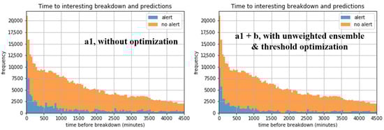
Figure 6.
Stacked histograms of failure alert presence/absence as a function of time before breakdown in the plastic domain, for stops due to plastic part being stuck in a core or cavity, for the best models.
5.3. Automotive Domain
5.3.1. Preliminary Observations
Over the 4.5-month analysis period, there is a total operation interval of approximately 4 months. During this time, a total of 35 crystallization threshold exceedance failure events, each occurring directly after a normal operating period, were identified according to the previously described method; in the RF case, 25 and 10 of them correspond to the training and test set, respectively. Sometimes, only a few timestamps intervene between two consecutive failure intervals.
Breakdowns of interest are typically preceded by the gradual increase in the water inlet temperature of the fifth booth after the valve for a couple of hours. By visually inspecting this trend prior to each relevant failure event, the values of the training parameters outlined in the next subsection were determined.
5.3.2. Tuned Training Arguments
All the training arguments that did not need to be common among the five base models constituting the ensemble model, which was optimized for each ensemble function, were tuned and are summarized in Table 4.
Table 4.
Tuned training arguments among the individual models of the ensemble in the automotive domain.
5.3.3. Forward Selection
For the model RF1 (as defined in Table 4), the eight selected features were trend, standard deviation, and frequency for periods 2 min, 2 min 13 s, 2 min 51 s, 4 min, 5 min, and 10 min. From the table, it follows that, regarding the other models IF and RF2-RF4, where forward selection was not intended, the input variables were 1, 11, 16, and 6 respectively.
5.3.4. Training Results
Similarly to the previous domains, Table 5 presents the best classification results from the intersection of the test sets of the base models in the automotive domain, for the considered 2 h forecasting horizon, which proved to be close to the average time difference between the beginning of the anomaly of interest and the crystallization failure, as will be shown later. Also in this domain, MCC is slightly improved compared to the conventional approach, but here false positives also decrease along with false negatives. All five base models play a significant role in the optimal ensemble, although IF, RF2, and RF3 seem more important. When using unweighted ensembles, with or without threshold optimization, the mean performs best as well.
Table 5.
Best confusion-matrix-based evaluation metrics demonstrating the impact of anomaly threshold and ensemble weights optimization in the automotive domain, for the 2 h forecasting horizon. The abbreviations are explained in Table 2. Underlined values are the best for the respective rows.
Similarly to the aluminum domain, Figure 7 demonstrates the reduction in false negatives, but also false positives, achieved through anomaly threshold optimization and ensemble methods, as detailed in Table 5. Each base model (without optimization) has its own disadvantages. IF perfectly detects high temperature, but does not recognize the anomalous upward trend on time, since it relies only on the raw value. The RF models detect the trend in a timely manner, but either miss some high values (RF3) or trigger false alarms before the real anomaly in trend (RF2). Instead, the optimized ensemble, which uses weighted averaging and threshold tuning, solves all these issues. More broadly, the overall improvement compared to the baseline method is visible in Figure 8.
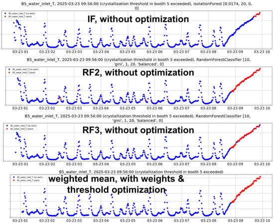
Figure 7.
Representative example of the behavior of the most critical raw variable (temperature) for forecasting in the automotive domain. The plot captures an entire interval with temperature below the crystallization threshold, which is exceeded just before and afterwards. The colors correspond to the binary predictions of the best models.
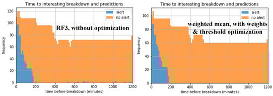
Figure 8.
Stacked histograms of failure alert presence/absence as a function of time before crystallization breakdown in the automotive domain, for the best models. In the ensemble case, the observations are fewer, because not all the features involved in all base models can be computed for some timestamps after lagging.
As previously promised, Table 6 demonstrates that DE is the most appropriate global optimizer of scipy for the simultaneous optimization of ensemble weights and the anomaly threshold in terms of convergence and computational complexity. The automotive domain was selected as an indicative example, since it involves the highest number of decision variables (5).
Table 6.
Comparative analysis of computational complexity among ensemble–threshold optimization methods in the automotive domain, for the 2 h forecasting horizon. Underlined values are the best for the respective columns.
6. Conclusions, Limitations, and Future Work
This work demonstrated how optimizing the failure probability/anomaly score threshold and the ensemble function parameters can be effectively combined to address the challenging task of timely anomaly detection for predictive maintenance, leading to improvements in the MCC, overall F-measure, and accuracy by a few percentage units. The algorithm was tested across multiple domains, showcasing its scalability across different industries, as well as highlighting both commonalities and differences in the implementations and their results. The findings from the aluminum domain suggest that the level of improvement may vary depending on the forecasting horizon. Indeed, the two main factors determining the improvement are, first, the distance between the forecasting horizon used for training/evaluation and the actual average time difference between the start of the anomaly and the associated failure, and, secondly, the complexity of the anomalous pattern in relation to the normal behavior, which determines the features to combine for accurate and timely anomaly detection only when needed. The observed variability in ensemble function performance across domains can be explained by the differences in failure manifestation, score calibration, and noise structure that are inherent to each industrial process. Weighted mean ensembles are effective when base models produce partially redundant yet complementary anomaly scores, allowing errors to compensate smoothly. However, in domains where failures are localized, rare, or inconsistently reflected across preprocessing pipelines, averaging may attenuate informative signals, leading to intermediate performance relative to individual models. In such cases, alternative ensemble functions that emphasize consensus or extreme responses (like the minimum) can yield superior discrimination. Importantly, these effects are further modulated by the jointly optimized decision threshold, as different aggregation schemes induce distinct score distributions and separability properties. The optimal value of the threshold depends on the ensemble function; for example, the minimum is expected to be associated with a lower threshold than the mean (weighted or not) or median, whereas the maximum is associated with higher. While the optimal ensemble–threshold configuration cannot be predicted analytically a priori, the proposed joint optimization framework enables systematic adaptation to domain-specific characteristics without manual tuning. Ensemble function and threshold optimization mainly decrease the false alerts, which is beneficial overall, even when it slightly increases their false absence when they should be raised. From the results, especially in the aluminum and automotive domains, it becomes obvious that there is no great margin for further improving performance, since alerts are more or less raised exactly while the actual anomaly preceding a failure of interest appears. The reason why MCC is far from one1 for any forecasting horizon is the uncertainty in the time before failure when the anomaly starts. Thus, it was considered pointless to test classifiers other than the efficient IF and RF. On the other hand, as results from the automotive case, using only one kind of classifier between the two is not always sufficient, because, since the one is unsupervised and the other supervised, they detect different characteristics determining anomalies. Finally, it is important to mention that, in our initial study using data from the aluminum domain, combining the classification method with regression models to forecast anomaly scores or raw values/features for earlier anomaly detection led to worse results compared to simply extending the classifier’s forecasting horizon.
The univariate optimization of MCC with regard to the threshold can be completed in just a few seconds using the Differential Evolution global optimizer with suitable parameter settings. This approach does not necessitate refitting the classifier for each objective function evaluation, as the failure probability or anomaly score is independent of the threshold, which only influences the percentage of alerts. In case the weighted mean ensemble function coefficients are also optimized, the ensemble anomaly scores are recomputed in every function evaluation, but again without refitting some classifier, since the base models remain the same. Simultaneous weight and threshold optimization takes some minutes and has linear complexity with regard to the number of timestamps. The main factor increasing the time complexity is the number of objective function evaluations. In our implementations, the values of this number are comparable between the T + wE and T + E cases, as shown in the relevant tables, but in the second case it would increase exponentially to the number of decision variables (or base models), so weighted mean coefficient optimization is more scalable. Indeed, as results from Algorithm 1, the number of function evaluations has complexity , where k, p, and m denote the number of iterations, population size, and problem dimension, respectively. Considering that the original DE paper [42] explicitly recommends a population size proportional to the problem dimension, and empirical evidence from benchmarking work on DE in the bibliography shows that the number of generations required for satisfactory convergence exhibits modest (often near-linear to sub-quadratic) complexity across a wide range of test problems [54], the number of function evaluations if k and p are considered functions of m has complexity . Furthermore, from preliminary experiments, it was proven that two-level optimization (firstly for the weights and secondly for the threshold) would require higher computational cost. Finally, the memory required is mainly due to the reading of the raw data and feature computation instead of training and optimization. As is well-known, generally, the IF and RF classifiers have time complexity and linear memory complexity with regard to the number of samples n, and these are independent of the number of input variables.
Regarding the limitations of the algorithm, sensor data alone are sufficient to run the models; however, ground truth equipment stop data are also required for evaluation purposes during the optimization of the predictive function, even for an unsupervised classifier, as without these, the relevance of the detected anomalies with upcoming interesting failures cannot be verified. Usually, stop information is not automatically registered and requires human input. If this is also unavailable, failure diagnosis methods based on the behavior of data during stops may be applied, such as clustering or Hidden Markov Models. In addition, different configurations and training may be needed for different components or failure reasons for optimal performance; otherwise, multi-class supervised methods may be tested, with the following disadvantages: severe class imbalance becomes harder to manage, probability estimates independence among failure types is lost, flexibility in feature relevance is reduced, cost-sensitive optimization gets harder, the addition of new failure types is not scalable (ir requires retraining the whole classifier, the performance of which can degrade on existing classes), evaluation and interpretation get more challenging, and, finally, overlapping or sequential failures are not supported.
In future research, the occasional automatic retraining of the models may be examined based on the time passed since the latest training or the evaluated deterioration of their performance based on a user-defined threshold for MCC or its decrease compared to the initial performance, since process conditions or the long-term behavior of the data may change from time to time. Furthermore, the optimization method may be further improved with smart automatic hyperparameter tuning approaches. Finally, in future work, a decentralized, parallel training of the base models constituting an ensemble may be examined.
Author Contributions
Conceptualization and project administration, D.I. and D.T.; methodology, investigation, writing—original draft preparation, and funding acquisition, N.K., V.T., and A.Z.; software, validation, formal analysis, data curation, writing—review and editing, visualization, and supervision, N.K.; and resources, not applicable. All authors have read and agreed to the published version of the manuscript.
Funding
This research and the APC were funded by the European Commission through the project HORIZON EUROPE-INNOVATION ACTIONS (IA)—grant number 101058453—FLEXIndustries. The opinions expressed in this paper are those of the authors and do not necessarily reflect the views of the European Commission.
Institutional Review Board Statement
Not applicable.
Informed Consent Statement
Not applicable.
Data Availability Statement
Restrictions apply to the availability of data from the industries due to privacy; data were obtained from their partners and are available from the authors with the permission of these partners.
Acknowledgments
The authors would like to thank the industrial partners for sharing data and communicating specifications.
Conflicts of Interest
The authors declare no conflicts of interest.
Abbreviations
The following abbreviations are used in this manuscript:
| AID | Arguments IDs |
| AUC-ROC | Area Under the Receiver Operating Characteristic |
| AUPRC | Area Under the Precision-Recall Curve |
| CNN | Convolutional Neural Network |
| DE | Differential Evolution |
| E | Ensemble with selection of functions among mean, median, maximum, and minimum |
| EFW | Ensemble function or weights of weighted mean |
| Fa% | F-measure of abnormal class (%) |
| Fh% | Harmonic mean of Pm% and Rm% |
| Fm% | Mean F-measure from classes (%) |
| FN | False Negatives |
| Fn% | F-measure of normal class (%) |
| FP | False Positives |
| GA | Genetic Algorithm |
| HMSPSO | Hybrid Multi-Swarm PSO |
| ID | Identity |
| IF | Isolation Forest |
| INISTA | International Conference on Innovations in Intelligent Systems and Applications |
| IoT | Internet of Things |
| LSTM | Long Short-Term Memory |
| MBHGA | Matrix-Based Hybrid Genetic Algorithm |
| MCC | Matthews Correlation Coefficient |
| nfev | Number of function evaluations |
| Pa% | Precision of abnormal class (%) |
| Pm% | Mean precision from classes (%) |
| Pn% | Precision of normal class (%) |
| PSO | Particle Swarm Optimization |
| Ra% | Recall of abnormal class (%) |
| RCGA-PSO | Real Coded GA-PSO |
| RF | Random Forest |
| Rm% | Mean recall from classes (%) |
| Rn% | Recall of normal class (%) |
| SHGO | Simplicial Homology Global Optimization |
| SMOTE | Synthetic Minority Over-sampling TEchnique |
| SVM | Support Vector Machine |
| T | Threshold optimization |
| TN | True Negatives |
| TP | True Positives |
| wE | Ensemble with weighted mean ensemble function and weights optimization |
References
- Kolokas, N.; Vafeiadis, T.; Ioannidis, D.; Tzovaras, D. Forecasting faults of industrial equipment using machine learning classifiers. In Proceedings of the International Conference on Innovations in Intelligent Systems and Applications (INISTA), Thessaloniki, Greece, 3–5 July 2018. [Google Scholar]
- Kolokas, N.; Tatsis, V.; Zacharaki, A.; Ioannidis, D.; Tzovaras, D. Improved Outlier Detection for Failure Forecasting using Anomaly Score Threshold Optimization and Ensemble Methods. In Proceedings of the International Conference on Innovations in Intelligent Systems and Applications (INISTA), Craiova, Romania, 4–6 September 2024. [Google Scholar]
- Kolokas, N.; Vafeiadis, T.; Ioannidis, D.; Tzovaras, D. Anomaly Detection in Aluminium Production with Unsupervised Machine Learning Classifiers. In Proceedings of the International Conference on Innovations in Intelligent Systems and Applications (INISTA), Sofia, Bulgaria, 3–5 July 2019. [Google Scholar]
- Kolokas, N.; Vafeiadis, T.; Ioannidis, D.; Tzovaras, D. A generic fault prognostics algorithm for manufacturing industries using unsupervised machine learning classifiers. Simul. Modell. Pract. Theory 2020, 103, 102109. [Google Scholar] [CrossRef]
- Mann, L.; Saxena, A.; Knapp, G.M. Statistical-based or condition-based preventive maintenance? J. Qual. Maint. Eng. 1995, 1, 46–59. [Google Scholar] [CrossRef]
- Yam, R.C.M.; Tse, P.W.; Li, L.; Tu, P. Intelligent predictive decision support systems for condition-based maintenance. Int. J. Adv. Manuf. Technol. 2001, 17, 383–391. [Google Scholar] [CrossRef]
- Hancock, J.; Johnson, J.M.; Khoshgoftaa, T.M. A comparative approach to threshold optimization for classifying imbalanced data. In Proceedings of the IEEE 8th International Conference on Collaboration and Internet Computing (CIC), Atlanta, GA, USA, 14–16 December 2022. [Google Scholar]
- Li, J.L.; Zhou, Y.F.; Ying, Z.Y.; Xu, H.; Li, Y.; Li, X. Anomaly detection based on isolated forests. In Advances in Artificial Intelligence and Security; Sun, X., Zhang, X., Xia, Z., Bertino, E., Eds.; Springer: Cham, Switzerland, 2021. [Google Scholar]
- Liu, T.; Ting, K.M.; Zhou, Z.-H. Isolation Forest. In Proceedings of the Eighth IEEE International Conference on Data Mining, Pisa, Italy, 15–19 December 2008. [Google Scholar]
- Wang, H.; Liang, Q.; Hancock, J.T.; Khoshgoftaar, T.M. Feature selection strategies: A comparative analysis of shap-value and importance-based methods. J. Big Data 2024, 11, 44. [Google Scholar] [CrossRef]
- Lakshmi, M.; Rajavikram, G.; Dattatreya, V.; Jyothi, B.S.; Patil, S.; Bhavsingh, M. Evaluating the isolation forest method for anomaly detection in software-defined networking security. J. Electr. Syst. 2023, 19, 279–297. [Google Scholar] [CrossRef]
- Vávra, J.; Hromada, M.; Lukáš, L.; Dworzecki, J. Adaptive anomaly detection system based on machine learning algorithms in an industrial control environment. Int. J. Crit. Infrastruct. Prot. 2021, 34, 100446. [Google Scholar] [CrossRef]
- Cao, C.; Chicco, D.; Hoffman, M.M. The MCC-F1 curve: A performance evaluation technique for binary classification. arXiv 2020, arXiv:2006.11278. [Google Scholar] [CrossRef]
- Lipton, Z.C.; Elkan, C.; Narayanaswamy, B. Thresholding Classifiers to Maximize F1 Score. arXiv 2014, arXiv:1402.1892. [Google Scholar]
- Hundman, K.; Constantinou, V.; Laporte, C.; Colwell, I.; Soderstrom, T. Detecting Spacecraft Anomalies Using LSTMs and Nonparametric Dynamic Thresholding. In Proceedings of the 24th ACM SIGKDD International Conference on Knowledge Discovery & Data Mining, London, UK, 19–23 August 2018; pp. 387–395. [Google Scholar]
- Yan, B.; Koyejo, S.; Zhong, K.; Ravikumar, P. Binary Classification with Karmic, Threshold-Quasi-Concave Metrics. In Proceedings of the 35th International Conference on Machine Learning, Stockholm, Sweden, 10–15 July 2018. [Google Scholar]
- Bougaham, A.; Frénay, B. Towards a Trustworthy Anomaly Detection for Critical Applications through Approximated Partial AUC Loss. arXiv 2025, arXiv:2502.11570. [Google Scholar] [CrossRef]
- Lau, M.; Seck, I.; Meliopoulos, A.P.; Lee, W.; Ndiaye, E.H. Revisiting Non-separable Binary Classification and its Applications in Anomaly Detection. arXiv 2023, arXiv:2312.01541. [Google Scholar] [CrossRef]
- Varalakshmi, S.; Premnath, S.; Yogalakshmi, V.; Kavitha, V.R.; Vimalarani, G. Design of IoT Network using Deep Learning-based Model for Anomaly Detection. In Proceedings of the Fifth International Conference on I-SMAC (IoT In Social, Mobile, Analytics and Cloud) (I-SMAC), Palladam, India, 11–13 November 2021; pp. 216–220. [Google Scholar]
- Chabchoub, Y.; Togbe, M.; Boly, A.; Chiky, R. An In-Depth Study and Improvement of Isolation Forest. IEEE Access 2022, 10, 10219–10237. [Google Scholar] [CrossRef]
- Kong, Q.; Xu, Y.; Wang, W.; Plumbley, M.D. Sound Event Detection of Weakly Labelled Data with CNN-Transformer and Automatic Threshold Optimization. IEEE/ACM Trans. Audio Speech Lang. Process. 2020, 28, 2450–2460. [Google Scholar] [CrossRef]
- Seman, L.O.; Aquino, L.S.; Stefenon, S.F.; Yow, K.-C.; Mariani, V.C.; Coehlo, L.d.S. Simultaneously anomaly detection and forecasting for predictive maintenance using a zero-cost differentiable architecture search-based network. Comput. Ind. Eng. 2025, 208, 111412. [Google Scholar] [CrossRef]
- Zhou, Z.-H. Ensemble Methods: Foundations and Algorithms; CRC Press: Boca Raton, FL, USA, 2025. [Google Scholar]
- Xin, R.; Liu, H.; Chen, P.; Zhao, Z. Robust and accurate performance anomaly detection and prediction for cloud applications: A novel ensemble learning-based framework. J. Cloud Comput. 2023, 12, 7. [Google Scholar] [CrossRef]
- Velásquez, D.; Pérez, E.; Oregui, X.; Artetxe, A.; Manteca, J.; Mansilla, J.E.; Toro, M.; Maiza, M.; Sierra, B. A hybrid machine-learning ensemble for anomaly detection in real-time industry 4.0 systems. IEEE Access 2022, 10, 72024–72036. [Google Scholar] [CrossRef]
- Chohra, A.; Shirani, P.; Karbab, E.B.; Debbabi, M. Chameleon: Optimized feature selection using particle swarm optimization and ensemble methods for network anomaly detection. Comput. Secur. 2022, 117, 102684. [Google Scholar] [CrossRef]
- Diop, A.; Emad, N.; Winter, T.; Hilia, M. Design of an Ensemble Learning Behavior Anomaly Detection Framework. 2023. Available online: https://hal.science/hal-04194528/ (accessed on 14 May 2024).
- Tyralis, H.; Papacharalampous, G.; Langousis, A. Super ensemble learning for daily streamflow forecasting: Large-scale demonstration and comparison with multiple machine learning algorithms. Neural Comput. Appl. 2021, 33, 3053–3068. [Google Scholar] [CrossRef]
- Tama, B.A.; Nkenyereye, L.; Islam, S.M.R.; Kwak, K.-S. An enhanced anomaly detection in web traffic using a stack of classifier ensemble. IEEE Access 2020, 8, 24120–24134. [Google Scholar] [CrossRef]
- Adeyemo, V.E.; Abdullah, A.; JhanJhi, N.Z.; Supramaniam, M.; Balogun, A.O. Ensemble and deep-learning methods for two-class and multi-attack anomaly intrusion detection: An empirical study. Int. J. Adv. Comput. Sci. Appl. 2019, 10, 520–528. [Google Scholar]
- Jian, C.; Ao, Y. Imbalanced fault diagnosis based on semi-supervised ensemble learning. J. Intell. Manuf. 2023, 34, 3143–3158. [Google Scholar] [CrossRef]
- Chawla, N.V.; Lazarevic, A.; Hall, L.O.; Bowyer, K.W. SMOTEBoost: Improving prediction of the minority class in boosting. In Proceedings of the European Conference on Principles of Data Mining and Knowledge Discovery, Cavtat-Dubrovnik, Croatia, 22–26 September 2003; pp. 107–119. [Google Scholar]
- Woźniak, M.; Grana, M.; Corchado, E. A survey of multiple classifier systems as hybrid systems. Inf. Fusion 2014, 16, 3–17. [Google Scholar] [CrossRef]
- Salehi, M.; Leckie, C.A.; Moshtaghi, M.; Vaithianathan, T. A Relevance Weighted Ensemble Model for Anomaly Detection in Switching Data Streams. In Proceedings of the Advances in Knowledge Discovery and Data Mining: 18th Pacific-Asia Conference (PAKDD), Tainan, Taiwan, 13–16 May 2014. [Google Scholar]
- Cabrera, J.B.D.; Gutiérrez, C.; Mehra, R.K. Ensemble methods for anomaly detection and distributed intrusion detection in Mobile Ad-Hoc Networks. Inf. Fusion 2008, 9, 96–119. [Google Scholar] [CrossRef]
- Zhong, Y.; Chen, W.; Wang, Z.; Chen, Y.; Wang, K.; Li, Y.; Yin, X.; Shi, X.; Yang, J.; Li, K. HELAD: A novel network anomaly detection model based on heterogeneous ensemble learning. Comput. Netw. 2020, 169, 107049. [Google Scholar] [CrossRef]
- Ünlü, R.; Xanthopoulos, P. A weighted framework for unsupervised ensemble learning based on internal quality measures. Ann. Oper. Res. 2019, 276, 229–247. [Google Scholar] [CrossRef]
- Liu, W.; Suzuki, Y.; Du, S. Ensemble learning algorithms based on easyensemble sampling for financial distress prediction. Ann. Oper. Res. 2025, 346, 2141–2172. [Google Scholar] [CrossRef]
- Cortes, C.; Vapnik, V. Support-vector networks. Mach. Learn. 1995, 20, 273–297. [Google Scholar] [CrossRef]
- Rousseeuw, P.J.; Driessen, K.V. A Fast Algorithm for the Minimum Covariance Determinant Estimator. Technometrics 1999, 41, 212–223. [Google Scholar] [CrossRef]
- Breunig, M.M.; Kriegel, H.-P.; Ng, R.T.; Sander, J. LOF: Identifying Density-based Local Outliers. In Proceedings of the ACM SIGMOD International Conference on Management of Data, Dallas, TX, USA, 15–18 May 2000. [Google Scholar]
- Storn, R.; Price, K. Differential evolution—A simple and efficient heuristic for global optimization over continuous spaces. J. Glob. Optim. 1997, 11, 341–359. [Google Scholar] [CrossRef]
- Mezura-Montes, E.; Velázquez-Reyes, J.; Coello Coello, C.A. A comparative study of differential evolution variants for global optimization. In Proceedings of the 8th Annual Conference on Genetic and Evolutionary Computation (GECCO), Seattle, WA, USA, 8–12 July 2006. [Google Scholar]
- Plevris, V.; Papadrakakis, M. A hybrid particle swarm-gradient algorithm for global structural optimization. Comput.-Aided Civ. Infrastruct. Eng. 2011, 26, 48–68. [Google Scholar] [CrossRef]
- Abbas, Q.; Ahmad, J.; Jabeen, H. A novel tournament selection based differential evolution variant for continuous optimization problems. Math. Probl. Eng. 2015, 2015, 205709. [Google Scholar] [CrossRef]
- Charalampakis, A.E.; Tsiatas, G.C. Critical evaluation of metaheuristic algorithms for weight minimization of truss structures. Front. Built Environ. 2019, 5, 113. [Google Scholar] [CrossRef]
- Wales, D.J.; Doye, J.P.K. Global Optimization by Basin-Hopping and the Lowest Energy Structures of Lennard-Jones Clusters Containing up to 110 Atoms. J. Phys. Chem. A 1997, 101, 5111–5116. [Google Scholar] [CrossRef]
- Xiang, Y.; Sun, D.Y.; Fan, W.; Gong, X.G. Generalized Simulated Annealing Algorithm and Its Application to the Thomson Model. Phys. Lett. A 1997, 233, 216–220. [Google Scholar] [CrossRef]
- Endres, S.C.; Sandrock, C.; Focke, W.W. A simplicial homology algorithm for Lipschitz optimisation. J. Glob. Optim. 2018, 72, 181–217. [Google Scholar] [CrossRef]
- Akopov, A.S.; Beklaryan, A.L.; Zhukova, A.A. Optimization of Characteristics for a Stochastic Agent-Based Model of Goods Exchange with the Use of Parallel Hybrid Genetic Algorithm. Cybern. Inf. Technol. 2023, 23, 87–104. [Google Scholar] [CrossRef]
- Akopov, A.S. A Hybrid Multi-Swarm Particle Swarm Optimization Algorithm for Solving Agent-Based Epidemiological Model. Cybern. Inf. Technol. 2025, 25, 59–77. [Google Scholar] [CrossRef]
- Chen, Y.; Li, L.; Xiao, J.; Yang, Y.; Liang, J.; Li, T. Particle swarm optimizer with crossover operation. Eng. Appl. Artif. Intell. 2018, 70, 159–169. [Google Scholar] [CrossRef]
- Akopov, A.S. MBHGA: A Matrix-Based Hybrid Genetic Algorithm for Solving an Agent-Based Model of Controlled Trade Interactions. IEEE Access 2025, 13, 26843–26863. [Google Scholar] [CrossRef]
- Apolloni, J.; García-Nieto, J.; Alba, E.; Leguizamón, G. Empirical evaluation of distributed Differential Evolution on standard benchmarks. Appl. Math. Comput. 2014, 236, 351–366. [Google Scholar] [CrossRef]


Disclaimer/Publisher’s Note: The statements, opinions and data contained in all publications are solely those of the individual author(s) and contributor(s) and not of MDPI and/or the editor(s). MDPI and/or the editor(s) disclaim responsibility for any injury to people or property resulting from any ideas, methods, instructions or products referred to in the content. |
© 2026 by the authors. Licensee MDPI, Basel, Switzerland. This article is an open access article distributed under the terms and conditions of the Creative Commons Attribution (CC BY) license.