Parametric Estimation and Analysis of Lifetime Models with Competing Risks Under Middle-Censored Data

Abstract

Middle-censoring is a general censoring mechanism. In middle-censoring, the exact lifetimes are observed only for a portion of the units and for others, we can only know the random interval within which the failure occurs. In this study, we focus on statistical inference for middle-censored data with competing risks. The latent failure times are assumed to be independent and follow Burr-XII distributions with distinct parameters. To begin with, we derive the maximum likelihood estimators for the unknown parameters, proving their existence and uniqueness. Additionally, asymptotic confidence intervals are constructed using the observed Fisher information matrix. Furthermore, Bayesian estimates under squared loss function and the corresponding highest posterior density intervals are obtained through the Gibbs sampling method. A simulation study is carried out to assess the performance of all proposed estimators. Lastly, an analysis for a practical dataset is provided to demonstrate the inferential processes developed.

1. Introduction

1.1. Middle-Censored Data and Competing Risks

Censoring occurs frequently in life test studies and cannot be completely avoided because of various practical constraints. Middle-censoring, a general censoring mechanism, was proposed by Jammalamadaka and Mangalam [1]. In middle-censoring, the precise failure time of the tested component cannot be detected when it occurs within a random interval. That is, the exact lifetimes of some units are observable, while for others we only know the intervals.

It is supposed that there are n identical units in a life test. The lifetimes of these units are defined as $T_1,T_2,\dots ,T_n$, and the i-th corresponding random interval is $[L_i,R_i]$. If $T_i\in [L_i,R_i]$, we cannot know the actual lifetime of the i-th unit, then ${\delta }_i=0$. Otherwise, ${\delta }_i=1$ denotes that the exact lifetime of the i-th unit can be observed directly. We can reorder the data, placing the complete data at the front, then the data can be described as:

$$(T_1,{\delta }_1),(T_2,{\delta }_2),\dots ,(T_{n_1},{\delta }_{n_1}),([L_{n_1+1},R_{n_1+1}],{\delta }_{n_1+1}),\dots ,([L_{n_1+n_2},R_{n_1+n_2}],{\delta }_{n_1+n_2}).$$

Jammalamadaka and Mangalam [1] not only put forward the middle-censoring scheme, but also developed an algorithm for obtaining the self-consistent estimator for the middle-censored data. The maximum likelihood estimator (MLE) in a non-parametric setting was also obtained. In addition, Jammalamadaka and Iyer [2] developed an approximation to the distribution function of the middle-censored data. Then, they also suggested a straightforward alternative estimator for the lifetime distribution function, analyzed its performance under middle-censored data, and established its consistency and weak convergence.

Moreover, several scholars have delved into middle-censored data within the parametric situation. Iyer et al. [3] considered a middle-censoring scheme in the case where the lifetime of the tested unit follows the exponential distribution. The maximum likelihood estimator was derived and its consistency and asymptotic properties were rigorously established. Additionally, the Bayes estimator was derived under a Gamma prior distribution. Davarzani and Parsia [4] studied a discrete set-up with middle-censored data, where the survival time, the left endpoint of the censoring interval, and the length of the interval are all variables modeled by geometric distributions. They derived the MLE of the unknown parameter using the EM algorithm. Bayesian estimator and the corresponding credible intervals were also obtained. Jammalamadaka and Bapat [5] developed the estimation under the middle-censoring paradigm in a multinomial distribution with k distinct possible outcomes. Abuzaid et al. [6] concentrated on the Weibull and exponential distributions to explore the robustness of their parameter estimates and discovered that estimations for middle-censoring exhibited greater robustness when contrasted with those for right censoring.

In practical applications, failure causes are typically pre-existing risk factors that may interact competitively. For example, in engineering reliability testing, environmental stressors such as temperature and humidity often compete to induce component failure. Statistical literature refers to this competitive failure mechanism as ‘competing risks’, emphasizing how multiple antecedent factors compete to be the first to exceed critical thresholds and cause system breakdown.

To consider the different reasons for failure, many studies combine competing risks with middle-censoring. Based on middle-censored data with two independent competing risks, Wang [7] explored various estimations of the parameter for exponential distribution. Ahmadi et al. [8] considered different estimations under middle-censored independent competing risks data with exponential distribution. Both the fix-point method and the EM algorithm were used to calculate the MLE. In addition, the Bayesian estimate under the Gamma prior was derived using both the Lindley’s approximation method and Gibbs sampling. The reconstruction of the censoring data was also explored. Wang et al. [9] investigated the dependent competing risks model based on middle-censored data by making use of the Marshall–Olkin bivariate Weibull distribution. They derived MLEs, midpoint approximation estimates, and asymptotic confidence intervals (ACIs) for the unknown parameters. They also considered the Bayesian estimates under the Gamma–Dirichlet prior by the acceptance–rejection sampling method. Davarzani et al. [10] analyzed a dependent middle-censoring model with the Marshall–Olkin bivariate exponential distribution.

In addition, other risk models have been explored. Sankaran and Prasad [11] proposed a proportional hazards regression framework to analyze middle-censored lifetime data with Weibull distribution. Rehman and Chandra [12] studied the cumulative incidence function by modeling the cause-specific hazard as a Weibull distribution for middle-censored survival data. Sankaran and Prasad [13] investigated an Exponentiated–Exponential regression model for middle-censored survival time analysis.

1.2. Burr-XII Distribution

The Burr XII distribution is a flexible and versatile distribution that is useful for modeling a wide range of data types. Its parameters allow it to exhibit different kurtosis and tail properties to adapt to different shapes, and the distribution has non-monotone hazard rates. In addition, both the cumulative and reliability function of the Burr-XII distribution have closed-form expressions, making it easier to compute percentiles and the likelihood function based on censored data, which makes it a valuable tool in statistical modeling and analysis [14].

A random variable X is said to follow the Burr $(a,b)$ distribution if its probability density function (PDF) and cumulative distribution function (CDF) are given by the following expressions, respectively:

$$f(t;a,b)=ab{t}^{b-1}{(1+t^b)}^{-(a+1)},t>0;a,b>0,$$

(1)

$$F(t;a,b)=1-{(1+t^b)}^{-a},t>0,$$

(2)

where $a,b$ are two positive shape parameters of the Burr-XII distribution.

In addition, the reliability and hazard rate function take the form as:

$$R(t;a,b)={(1+t^b)}^{-a},t>0,$$

(3)

$$h(t;a,b)={\displaystyle \frac{ab{t}^{b-1}}{1+t^b}},t>0.$$

(4)

In the density plots in Figure 1, it can be observed that when $b\le$ 1, the density curve is strictly decreasing, while the Burr-XII distribution density curve is unimodal when $b>1$ and at this time, a larger a corresponds to a higher peak height of the curve.

Figure 1. PDF plots of Burr-XII distribution under various parameter configurations.

In addition, Figure 2 shows the hazard rate function plots. As shown in the picture, when $b\le 1$, the hazard rate function decreases with t becoming larger, while the plot has a single peak when $b>1$. The peak is higher when the value of parameter a becomes larger.

Figure 2. Hazard rate function plots of Burr-XII distribution under various parameter configurations.

Recently, owing to its versatility in applied contexts like reliability analysis, quality assurance, and quantum systems, the Burr-XII distribution has attracted significant interest from several scholars.

There are many studies for Burr-XII distribution based on various life tests and censoring schemes. Soliman [15] derived both the MLE and Bayesian estimation approaches for the Burr-XII distribution parameters under progressive Type-II censoring scenarios. Yan et al. [16] exploited the MLE and Bayes estimation within an improved adaptive Type-II progressive censoring framework under the Burr-XII distribution. Du and Gui [17] investigated the Burr-XII distribution in competitive risk modeling under adaptive Type-II progressive censoring. Bayesian point estimates under various loss functions and the corresponding highest posterior density credible intervals were obtained through MCMC simulations.

Although there are a large amount of statistical inferences related to the Burr-XII distribution along with censored data, they mainly focused on Type-II censoring or other progressive censoring schemes, and studies on the Burr-XII distribution under middle censoring are currently limited. Abuzaid [18] analyzed middle-censored data from the Burr-XII distribution. MLEs of two parameters were obtained, and Bayesian inferences under a Gamma prior were established through the application of Lindley’s approximation technique. However, it did not consider the failure reasons. Thus, based on that, in this paper we will introduce independent competing risks to study the middle-censored data under Burr-XII distribution.

To our knowledge, no existing studies have comprehensively investigated the parameter-estimation challenges for Burr-XII distributions considering both middle-censored data and competing risks models. In this paper, we combine the competing risks with middle-censored data to address the parameter-estimation problems for the Burr-XII distribution. Compared to [17], we introduce a new censoring scheme and consider different numbers of failure causes. Different from [18], we introduce a competing risks model to the analysis framework.

In this paper, we use the perspective of latent failure times for a competing risk model suggested by Cox [19]. An analysis of the independent competing risks model is conducted within a middle-censoring scenario. It is assumed that each latent failure time variable follows the Burr-XII distribution. In Section 2, we make some reasonable assumptions for our model. In Section 3, we prove that the MLEs exist uniquely, implementing both optimization techniques and the EM algorithm to obtain them. In addition, we derive ACIs in accordance with the properties of MLEs. In Section 4, we obtain the Bayesian estimators under exponential and Gamma prior distributions using Gibbs sampling, and HPD credible intervals are also constructed. Section 5 presents the simulation results to validate estimator performance and applies the model to a practical dataset to demonstrate the application value of our model.

2. Model Assumption and Notation

Assume that $n\in \mathbb{N}$ homogeneous units are assigned to a lifetime test. For each unit, there are s failure causes. We suppose that these s latent failure times are mutually independent and conform to the Burr-XII distribution.

Thus, define $T_i$ as the exact lifetime of the i-th tested unit, and 

$$T_i=min\left\{X_{i1},X_{i2},\dots ,X_{is}\right\},$$

where $X_{ij}$ represents the random variable corresponding to the j-th latent failure cause. Moreover, $X_{i1},X_{i2},\dots ,X_{is}$ are independent of each other. We assume that $X_{ij},j=1,2,\dots ,s$ follow the Burr-XII distributions with the same second parameter ($b>0$) and different first parameters ($a_1,a_2,\dots ,a_s>0$). The PDF and CDF of $X_{ij}$ are presented as follows, respectively:

$$f_j(t;a_j,b)=a_{j}b{t}^{b-1}{(1+t^b)}^{-(a_j+1)},t>0;a_j,b>0,$$

(5)

and

$$F_j(t;a_j,b)=1-{(1+t^b)}^{-a_j},t>0,$$

(6)

where $a_j$ and b are unknown parameters to be estimated and they are all positive, $j=1,2,\dots ,s$.

As exhibited in Figure 1, the parameter b affects the overall shape of the density curve. For different failure causes of the same product, it is reasonable to assume that the distributions share the same parameter b. The assumption that the potential failure distributions share a common parameter while differing in the other has been widely used in previous studies on competing risks data, such as [20,21].

Additionally, we use $D_i$ to denote the failure cause. $D_i=j$ if the i-th unit has failed as a result of the j-th failure cause. We suppose that $\left\{X_{i1},X_{i2},\dots ,X_{is}\right\}$ are independent and cannot be observed directly, while $T_i$ and $D_i$ can be observed if the data are not censored. Therefore, taking into account the competing risks data under a middle-censoring framework, we consider a corresponding random censoring interval $[L_i,R_i]$ for the i-th tested unit, and the interval is independent of its actual lifetime $T_i$. That is,

$$(Y_i,D_i,{\delta }_i)=\left\{\begin{array}{cc}(T_i,D_i,1)\hfill & \mathrm{if}{T}_i\notin [L_i,R_i],\hfill \\ \left([L_i,R_i],D_i,0\right)\hfill & \mathrm{if}{T}_i\in [L_i,R_i].\hfill \end{array}\right.$$

We suppose $L_i$ and $R_i-L_i$ are also independent and exponentially distributed with known parameters.

Through the independence of $X_{i1},X_{i2},\dots ,X_{is}$, the joint PDF and CDF of lifetime with its corresponding cause $(T,D)$ are concluded as follows:

$$f_{T,D}(t,j;\mathbf{a},b)=f_j(t;a_j,b)\prod _{k=1,k\ne j}^s(1-F_k(t;a_k,b))=a_{j}b{t}^{b-1}{(1+t^b)}^{-(a^{*}+1)},$$

(7)

where $\mathbf{a}=(a_1,a_2,\dots ,a_s)$ and $a^{*}={\sum }_{j=1}^s{a}_j$.

Through integration, we derive:

$$F_{T,D}(t,j;\mathbf{a},b)={\displaystyle \frac{a_j}{a^{*}}}[1-{(1+t^b)}^{-a^{*}}].$$

(8)

To simplify the notation, we will replace $F_{T,D}(t,j;\mathbf{a},b)$ and $f_{T,D}(t,j;\mathbf{a},b)$ with $F(t,j;\mathbf{a},b)$ and $f(t,j;\mathbf{a},b)$, respectively, in the following text.

3. Frequentist Estimation

This section begins by deriving the likelihood function and establishing the existence and uniqueness of MLEs of the model parameters. Both optimization-based methods and the EM algorithm are then employed to compute these estimates. ACIs are constructed using the Fisher information matrix.

3.1. Maximum Likelihood Estimators

For simplicity, according to the approach in [8], after reordering the data, the sample is partitioned such that the first $n_1$ data items are not censored, and the subsequent $n_2$ data items are middle-censored. Thus, our data can be written as:

$$\{(T_1,D_1),\dots ,(T_{n_1},D_{n_1}),([L_{n_1+1},R_{n_1+1}],D_{n_1+1}),\dots ,([L_{n_1+1},R_{n_1+n_2}],D_{n_1+n_2})\}.$$

Let $data$ represent the observed sample data in the form mentioned above. Based on the sample data, the likelihood function can be derived through (7) and (8) as follows:

$$\begin{array}{c}\hfill L(\mathbf{a},b;data)\propto \prod _{j=1}^s\prod _{i=1}^{n_1}{(f(t_i,j;\mathbf{a},b))}^{I(D_i=j)}\prod _{j=1}^s\prod _{i=n_1+1}^{n_1+n_2}{(F(r_i,j;\mathbf{a},b)-F(l_i,j;\mathbf{a},b))}^{I(D_i=j)}\\ \hfill =b^{n_1}{({\displaystyle \frac{1}{a^{*}}})}^{n_2}\prod _{j=1}^s{a}_j^{m_j}\prod _{i=1}^{n_1}\left[t_i^{b-1}{(1+t_i^b)}^{-(a^{*}+1)}\right]\prod _{i=n_1+1}^{n_1+n_2}[{(1+l_i^b)}^{-a^{*}}-{(1+r_i^b)}^{-a^{*}}]\end{array}$$

(9)

where symbol ∝ denotes ’proportional to’,

$$I(D_i=j)=\left\{\begin{array}{cc}\hfill 1& \hfill \mathrm{if}{D}_i=j,\hfill \\ \hfill 0& \hfill \mathrm{Otherwise},\hfill \end{array}\right.$$

and $m_j={\sum }_{i=1}^{n}I(D_i=j)$, which equals the number of the items that have failed attributed to the j-th latent risk. For simplicity, we use $L(\mathbf{a},b)$ to replace $L(\mathbf{a},b;data)$.

Through (9), the log-likelihood function takes the form:

$$\begin{array}{c}\hfill lnL(\mathbf{a},b)=n_{1}lnb-n_{2}ln{a}^{*}+\sum _{j=1}^s{m}_{j}ln{a}_j+(b-1)\sum _{i=1}^{n_1}ln{t}_i\\ \hfill -(a^{*}+1)\sum _{i=1}^{n_1}ln(1+t_i^b)+\sum _{i=n_1+1}^{n_1+n_2}ln[{(1+l_i^b)}^{-a^{*}}-{(1+r_i^b)}^{-a^{*}}].\end{array}$$

(10)

To solve for the MLEs, we set the first-order partial derivatives of function $lnL(\mathbf{a},\mathbf{b})$ with respect to all unknown parameters $a_1,a_2,\dots ,a_s$ and b to 0, respectively. Consequently, the corresponding likelihood equations are given by:

$$\begin{array}{c}\hfill {\displaystyle \frac{\partial lnL(\mathbf{a},b)}{\partial a_j}}={\displaystyle \frac{m_j}{a_j}}-{\displaystyle \frac{n_2}{a^{*}}}-\sum _{i=1}^{n_1}ln(1+t_i^b)+K_1=0,j=1,2,3,\dots ,s,\end{array}$$

(11)

$$\begin{array}{c}\hfill {\displaystyle \frac{\partial lnL(\mathbf{a},b)}{\partial b}}={\displaystyle \frac{n_1}{b}}+\sum _{i=1}^{n_1}ln{t}_i-(a^{*}+1)\sum _{i=1}^{n_1}{\displaystyle \frac{t_i^{b}ln{t}_i}{1+t_i^b}}+a^{*}{K}_2=0,\end{array}$$

(12)

where

$$K_1=\sum _{i=n_1+1}^{n_1+n_2}{\displaystyle \frac{{(1+r_i^b)}^{-a^{*}}ln(1+r_i^b)-{(1+l_i^b)}^{-a^{*}}ln(1+l_i^b)}{{(1+l_i^b)}^{-a^{*}}-{(1+r_i^b)}^{-a^{*}}}},$$

and

$$K_2=\sum _{i=n_1+1}^{n_1+n_2}{\displaystyle \frac{r_i^b{(1+r_i^b)}^{-(a^{*}+1)}ln{r}_i-l_i^b{(1+l_i^b)}^{-(a^{*}+1)}ln{l}_i}{{(1+l_i^b)}^{-a^{*}}-{(1+r_i^b)}^{-a^{*}}}}.$$

For $j=1,2,\dots ,s$, we determine, respectively, the MLEs of $a_j$ and $a^{*}$ as $\widehat{a_j}$ and $\widehat{a^{*}}$, and the MLE of b is expressed as $\widehat{b}$. Based on (11), we can derive that ${\displaystyle \frac{m_1}{a_1}}={\displaystyle \frac{m_2}{a_2}}=\dots ={\displaystyle \frac{m_s}{a_s}}$. Thus,

$${\displaystyle \frac{\widehat{a_j}}{m_j}}={\displaystyle \frac{\widehat{a^{*}}}{n}},j=1,2,\dots ,s.$$

(13)

Before obtaining the solution through (11)–(13), the uniqueness and existence of solutions to the likelihood equations require verification.

Theorem 1.

For competing risks and middle-censored data following the Burr-XII distribution, when parameter b is known, the MLEs of parameters $a_1,a_2,\dots ,a_s$ are always existent and unique.

Proof. 

Through (11)–(13), the likelihood equations are equivalent to the following:

$$\left\{\begin{array}{c}{d}_1(a^{*},b)={\displaystyle \frac{n_1}{a^{*}}}-\sum _{i=1}^{n_1}ln(1+t_i^b)+\sum _{i=n_1+1}^{n_1+n_2}{\displaystyle \frac{{\psi }_{r_i}^{-a^{*}}ln{\psi }_{r_i}-{({\psi }_{l_i})}^{-a^{*}}ln{\psi }_{l_i}}{{\psi }_{l_i}^{-a^{*}}-{\psi }_{r_i}^{-a^{*}}}}=0\hfill \\ d_2(a^{*},b)={\displaystyle \frac{n_1}{b}}+\sum _{i=1}^{n_1}ln{t}_i-(a^{*}+1)\sum _{i=1}^{n_1}{\displaystyle \frac{t_i^{b}ln{t}_i}{1+t_i^b}}+a^{*}\sum _{i=n_1+1}^{n_1+n_2}{\displaystyle \frac{r_i^b{\psi }_{r_i}^{-(a^{*}+1)}ln{r}_i-l_i^b{\psi }_{l_i}^{-(a^{*}+1)}ln{l}_i}{{\psi }_{l_i}^{-a^{*}}-{\psi }_{r_i}^{-a^{*}}}}=0\hfill \end{array}\right.,$$

(14)

where ${\psi }_{r_i}=1+r_i^b$ and ${\psi }_{l_i}=1+l_i^b$. Therefore,

$${\displaystyle \frac{\partial d_1(a^{*},b)}{\partial a^{*}}}=-{\displaystyle \frac{n_1}{{a^{*}}^2}}-B,$$

(15)

where

$$B=\sum _{i=n_1+1}^{n_1+n_2}{\displaystyle \frac{{\psi }_{r_i}^{-a^{*}}{\psi }_{l_i}^{-a^{*}}{(ln{\psi }_{r_i}-ln{\psi }_{l_i})}^2}{{({\psi }_{l_i}^{-a^{*}}-{\psi }_{r_i}^{-a^{*}})}^2}}.$$

When b is a known constant, we just obtain the solution of $d_1(a^{*},b)=0$ to obtain $\widehat{a^{*}}$. It is obvious that ${\displaystyle \frac{\partial d_1(a^{*},b)}{\partial a^{*}}}<0$, and that

$$\left\{\begin{array}{c}\underset{a^{*}\to 0}{lim}{d}_1(a^{*},b)=+\infty \hfill \\ \underset{a^{*}\to +\infty }{lim}{d}_1(a^{*},b)=-\sum _{i=1}^{n_1}ln(1+t_i^b)-\sum _{i=n_1+1}^{n_1+n_2}ln{\psi }_{l_i}<0\hfill \end{array}\right.,$$

(16)

so $d_1(a^{*},b)$ is monotonically decreasing with respect to $a^{*}$, and takes both positive and negative values, which indicates the existence and uniqueness of the zero point $\widehat{a^{*}}$. Therefore, through (13), we can conclude that when b is fixed, for parameters $a_1,a_2,\dots ,a_s$, their MLEs always exist and are unique and finite.    □

Theorem 2.

For competing risks and middle-censored data following the Burr-XII distribution, in the case that $a_1,a_2,\dots ,a_s$ and b are all unknown, when there exists i such that $t_i<1$, the MLEs $\widehat{a_1},\widehat{a_2},\dots ,\widehat{a_2}$ and $\widehat{b}$ all exist and are unique.

Proof. 

According to (9), the joint likelihood function is expressed as:

$$L(\mathbf{a},b)\propto \prod _{j=1}^s\prod _{i=1}^{n_1}{(f(t_i,j;\mathbf{a},b))}^{I(D_i=j)}\prod _{j=1}^s\prod _{i=n_1+1}^{n_1+n_2}{(F(r_i,j;\mathbf{a},b)-F(l_i,j;\mathbf{a},b))}^{I(D_i=j)},$$

in accordance with the Lagrange mean-value theorem, there is a ${\xi }_i\in [L_i,R_i]$ satisfying $[F(r_i,j;\mathbf{a},b)-F(l_i,j;\mathbf{a},b)]=(R_i-L_i)f({\xi }_i,j;\mathbf{a},b)$.

So we just need to prove that when the data are uncensored, the MLEs of the parameters $a^{*}$ and b are existent and unique.

Through (24), and for $i>n_1$, for convenience, we substitute $t_i^{*}$ with $t_i$, then we can obtain that

$$\widehat{a^{*}}=n/\sum _{i=1}^{n}ln(1+t_i^b).$$

(17)

Then, $\widehat{b}$ is the solution of the equation given as follows:

$$z(b)={\displaystyle \frac{n}{b}}+\sum _{i=1}^{n}ln{t}_i-({\displaystyle \frac{n}{{\sum }_{i=1}^{n}ln(1+t_i^b)}}+1)\sum _{i=1}^n{\displaystyle \frac{t_i^{b}ln{t}_i}{1+t_i^b}}=0.$$

(18)

We can derive the derivative of $z(b)$ as follows:

$$z^{\prime }(b)=-{\displaystyle \frac{n}{b^2}}-{\displaystyle \frac{n}{{({\sum }_{i=1}^{n}ln(1+t_i^b))}^2}}{(\sum _{i=1}^n{\displaystyle \frac{t_i^{b}ln{t}_i}{1+t_i^b}})}^2-{\displaystyle \frac{n}{{\sum }_{i=1}^{n}ln(1+t_i^b)}}\sum _{i=1}^n{\displaystyle \frac{t_i^b{(ln{t}_i)}^2}{{(1+t_i^b)}^2}}<0,$$

(19)

and it is obvious that

$$\left\{\begin{array}{c}\underset{b\to 0}{lim}z(b)=+\infty \hfill \\ \underset{b\to +\infty }{lim}z(b)=\underset{b\to +\infty }{lim}{z}_1(b)+\underset{b\to +\infty }{lim}{z}_2(b),\hfill \end{array}\right.$$

where $z_1(b)=-{\displaystyle \frac{n}{{\sum }_{i=1}^{n}ln(1+t_i^b)}}{\sum }_{i=1}^n{\displaystyle \frac{t_i^{b}ln{t}_i}{1+t_i^b}}$ and $z_2(b)={\sum }_{i=1}^n{\displaystyle \frac{ln{t}_i}{1+t_i^b}}$.

For each $t_i,i=1,2,\dots ,n$, if $t_i<1$, $\underset{b\to +\infty }{lim}{\displaystyle \frac{ln{t}_i}{1+t_i^b}}=ln{t}_i<0$ and if $t_i\ge 1$,$\underset{b\to +\infty }{lim}{\displaystyle \frac{ln{t}_i}{1+t_i^b}}=0$, so $\underset{b\to +\infty }{lim}{z}_2(b)<0$ when there exists an i such that $t_i<1$. Moreover, it is simple to derive that $\underset{b\to +\infty }{lim}{z}_1(b)\le 0$. Thus, $\underset{b\to +\infty }{lim}z(b)<0$. Subsequently, we are able to prove that the function $z(b)$ is strictly monotonically decreasing on the interval $(0,+\infty )$. Moreover, as b varies from 0 to $+\infty$, the sign of the function shifts from positive to negative. Therefore, the solution of $z(b)=0$ exists and is unique, which indicates that $\widehat{b}$ is unique, and through (17), the uniqueness of $\widehat{a^{*}}$ can be proved. Consequently, the presence and uniqueness of the MLEs of unknown parameters $a_1,a_2,\dots ,a_s$ are demonstrated.    □

Remark 1.

When using our model to deal with data, to ensure the existence, we just need to appropriately transform the units of physical quantities in the sample data to guarantee that there exists $t_i<1$.

Since the explicit solution of the equations is difficult to obtain, we use certain iterative algorithms to calculate the MLEs of unknown parameters. In this paper, in order to maximize $lnL(\mathbf{a},b)$, we use the optim function in R language (version 4.3.2).

3.2. EM Algorithm

Given that explicit expressions for $\widehat{a_j}$ and $\widehat{b}$ are unavailable, the EM algorithm is considered and employed to find the MLEs. Incomplete data scenarios are typically addressed using the EM algorithm, which is first formulated by Dempster et al. [22].

Define $t_i^{*}$ as the exact survival time of the unit that falls within the interval [$l_i$,$r_i$], $i=n_1+1$,...,$n_1+n_2$.

Based on the complete data ($t_1,t_2,\dots ,t_{n_1},t_{n_1+1}^{*},\dots ,t_{n_1+n_2}^{*}$), we can derive the log-likelihood function, which is expressed as:

$$\begin{array}{c}\hfill ln{L}_C(\mathbf{a},b)=\sum _{j=1}^s{m}_{j}ln{a}_j+nlnb+(b-1)(\sum _{i=1}^{n_1}ln{t}_i+\sum _{i=n_1+1}^{n_1+n_2}ln{t}_i^{*})\\ \hfill -(a^{*}+1)(\sum _{i=1}^{n_1}ln(1+t_i^b)+\sum _{i=n_1+1}^{n_1+n_2}ln(1+{t_i^{*}}^b)),\end{array}$$

(20)

then by setting the derivatives of $ln{L}_C(\mathbf{a},b)$ with respect to $a_j$ and b to 0, we can obtain:

$${\displaystyle \frac{\partial ln{L}_c(\mathbf{a},b)}{\partial a_j}}={\displaystyle \frac{m_j}{a_j}}-(\sum _{i=1}^{n_1}ln(1+t_i^b)+\sum _{i=n_1+1}^{n_1+n_2}ln(1+{t_i^{*}}^b))=0,j=1,2,\dots ,s,$$

(21)

$$\begin{array}{c}\hfill {\displaystyle \frac{\partial ln{L}_c(\mathbf{a},b)}{\partial b}}={\displaystyle \frac{n}{b}}+(\sum _{i=1}^{n_1}ln{t}_i+\sum _{i=n_1+1}^{n_1+n_2}ln{t}_i^{*})\\ \hfill -(a^{*}+1)(\sum _{i=1}^{n_1}{\displaystyle \frac{t_i^{b}ln{t}_i}{1+t_i^b}}+\sum _{i=n_1+1}^{n_1+n_2}{\displaystyle \frac{{(t_i^{*})}^{b}ln{t}_i^{*}}{1+{t_i^{*}}^b}})=0.\end{array}$$

(22)

Through Equation (21), we can obtain that

$${\displaystyle \frac{m_j}{\widehat{a_j}}}={\displaystyle \frac{n}{\widehat{a^{*}}}},j=1,2,\dots ,s,$$

(23)

and we can derive the system of equations:

$$\left\{\begin{array}{c}{\displaystyle \frac{n}{a^{*}}}-(\sum _{i=1}^{n_1}ln(1+t_i^b)+\sum _{i=n_1+1}^{n_1+n_2}ln(1+{t_i^{*}}^b))=0\hfill \\ {\displaystyle \frac{n}{b}}+(\sum _{i=1}^{n_1}ln{t}_i+\sum _{i=n_1+1}^{n_1+n_2}ln{t}_i^{*})-(a^{*}+1)(\sum _{i=1}^{n_1}{\displaystyle \frac{t_i^{b}ln{t}_i}{1+t_i^b}}+\sum _{i=n_1+1}^{n_1+n_2}{\displaystyle \frac{{t_i^{*}}^{b}ln{t}_i^{*}}{1+{t_i^{*}}^b}})=0\hfill \end{array}\right..$$

(24)

For conciseness, we define the conditional expectations as follows:

$$E_{\mathbf{a},b}(ln{T}_i|T_i\in [l_i,r_i],D_i=d_i)={\int }_{l_i}^{r_i}{\displaystyle \frac{lnt\times f(t,d_i;\mathbf{a},b)}{F(r_i,d_i;\mathbf{a},b)-F(l_i,d_i;\mathbf{a},b)}}dt,$$

$$E_{\mathbf{a},b}(ln(1+T_i^b)|T_i\in [l_i,r_i],D_i=d_i)={\int }_{l_i}^{r_i}{\displaystyle \frac{ln(1+t^b)\times f(t,d_i;\mathbf{a},b)}{F(r_i,d_i;\mathbf{a},b)-F(l_i,d_i;\mathbf{a},b)}}dt,$$

$$E_{\mathbf{a},b}({\displaystyle \frac{T_i^{b}ln{T}_i}{1+T_i^b}}|T_i\in [l_i,r_i],D_i=d_i)={\int }_{l_i}^{r_i}{\displaystyle \frac{t^{b}lnt}{1+t^b}}\times {\displaystyle \frac{f(t,d_i;\mathbf{a},b)}{F(r_i,d_i;\mathbf{a},b)-F(l_i,d_i;\mathbf{a},b)}}dt,$$

where the expressions of $f(t,d_i;\mathbf{a},b)$ and $F(t,d_i;\mathbf{a},b)$ can be seen in (7) and (8).

In each iteration, to perform the E-step, we need to calculate the expectations using the parameter values obtained from the previous iteration by numerical integration methods. For notational convenience, we introduce the symbols as follows:

• $E_{1,i}^{(k)}=E_{{\mathbf{a}}^{(k-1)},b^{(k-1)}}(ln{T}_i|T_i\in [l_i,r_i],D_i=d_i)$,
• $E_{2,i}^{(k)}=E_{{\mathbf{a}}^{(k-1)},b^{(k-1)}}(ln(1+T_i^b)|T_i\in [l_i,r_i],D_i=d_i)$,
• $E_{3,i}^{(k)}=E_{{\mathbf{a}}^{(k-1)},b^{(k-1)}}({\displaystyle \frac{T_i^{b}ln{T}_i}{1+T_i^b}}|T_i\in [l_i,r_i],D_i=d_i)$,

where $i=n_1+1,n_1+2,\dots ,n_1+n_2$. And for those uncensored data, we define:

$$F_{1,i}^{(k)}=ln{t}_i,F_{2,i}^{(k)}=ln(1+t_i^{b^{(k-1)}}),F_{3,i}^{(k)}={\displaystyle \frac{t_i^{b^{(k-1)}}ln{t}_i}{1+t_i^{b^{(k-1)}}}},$$

where $i=1,2,\dots ,n_1$.

When performing the M-step during the iteration process, for the purpose of maximizing the pseudo log-likelihood function $ln{L}_C(\mathbf{a},b)$ based on the complete data, through (24), we can derive that

$${a^{*}}^{(k)}=n{(\sum _{i=1}^{n_1}{F}_{2,i}^{(k)}+\sum _{i=n_1+1}^{n_1+n_2}{E}_{2,i}^{(k)})}^{-1},$$

(25)

and

$$b^{(k)}=n{[({a^{*}}^{(k)}+1)(\sum _{i=1}^{n_1}{F}_{3,i}^{(k)}+\sum _{i=n_1+1}^{n_1+n_2}{E}_{3,i}^{(k)})-(\sum _{i=1}^{n_1}{F}_{1,i}^{(k)}+\sum _{i=n_1+1}^{n_1+n_2}{E}_{1,i}^{(k)})]}^{-1}.$$

(26)

In addition, we say the process converges when

$$|a_j^{(k+1)}-a_j^{(k)})|<ϵ,j=1,2,\dots ,s,$$

and

$$|b^{(k+1)}-b^{(k)})|<ϵ,$$

where $ϵ$ represents the tolerance threshold fixed in advance, and proper values of $ϵ$ need to be obtained by numerical tests. Based on the above, the sequential steps of the EM algorithm are expressed in Algorithm 1 systematically.

Algorithm 1 The EM algorithm for obtaining MLEs under middle-censored data with competitive risks

1: Input: $data$, initial parameter ${a^{*}}^{(0)}$, $b^{(0)}$ and $a_j^{(0)}={\displaystyle \frac{m_j{a^{*}}^{(0)}}{n}}$   2: Initialization:  $k=0$   3: while not converged do   4:       E-step (Expectation step):   5:       Under the current parameter estimate $({\mathbf{a}}^{(k-1)},b^{(k-1)})$, calculate the expectations: $$E_{1,i}^{(k)},E_{2,i}^{(k)},E_{3,i}^{(k)}fori=n_1+1,n_1+2,\dots ,n_1+n_2$$ $$F_{1,i}^{(k)},F_{2,i}^{(k)},F_{3,i}^{(k)}fori=1,2,\dots ,n_1$$   6:       M-step (Maximization step):   7:       Update the parameter estimates by using Equations (25) and (26)   8:       $k=k+1$   9: end while 10: Output: Estimated parameter ${a_j^{*}}^{(k)}$ and $b^{(k)}$

3.3. Asymptotic Confidence Intervals

To obtain the ACIs of the unknown parameters $a_j,j=1,2,\dots ,s$ and b, we use the Fisher information matrix introduced in [23], and the matrix is derived by calculating the corresponding second-order partial derivatives. Then, we present the Fisher information matrix as:

$${\displaystyle \frac{{\partial }^{2}lnL(\mathbf{a},b)}{\partial a_k\partial a_j}}=\left\{\begin{array}{cc}{\displaystyle \frac{-m_j}{a_j^2}}+{\displaystyle \frac{n_2}{{a^{*}}^2}}-B\hfill & \mathrm{if}k=j\hfill \\ {\displaystyle \frac{n_2}{{a^{*}}^2}}-B\hfill & \mathrm{if}k\ne j\hfill \end{array}\right.k,j=1,2,\dots ,s,$$

(27)

where

$$B=\sum _{i=n_1+1}^{n_1+n_2}{\displaystyle \frac{{\psi }_{r_i}^{-a^{*}}{\psi }_{l_i}^{-a^{*}}{[ln{\psi }_{r_i}-ln{\psi }_{l_i}]}^2}{{({\psi }_{l_i}^{-a^{*}}-{\psi }_{r_i}^{-a^{*}})}^2}},$$

${\psi }_{l_i}=1+l_i^b$, and ${\psi }_{r_i}=1+r_i^b$. In addition,

$${\displaystyle \frac{{\partial }^{2}lnL(\mathbf{a},b)}{\partial a_j\partial b}}=-\sum _{i=1}^{n_1}{\displaystyle \frac{t_i^{b}ln{t}_i}{1+t_i^b}}+C+D,j=1,2,\dots ,s,$$

(28)

where

$$C=\sum _{i=n_1+1}^{n_1+n_2}{\displaystyle \frac{r_i^b{\psi }_{r_i}^{-(a^{*}+1)}ln{r}_i-l_i^b{\psi }_{l_i}^{-(a^{*}+1)}ln{l}_i}{{\psi }_{l_i}^{-a^{*}}-{\psi }_{r_i}^{-a^{*}}}},$$

$$D=a^{*}\sum _{i=n_1+1}^{n_1+n_2}{({\psi }_{r_i}{\psi }_{l_i})}^{-(a^{*}+1)}(ln{\psi }_{r_i}-ln{\psi }_{l_i}){\displaystyle \frac{{\psi }_{r_i}{l}_i^{b}ln{l}_i-{\psi }_{l_i}{r}_i^{b}ln{r}_i}{{({\psi }_{l_i}^{-a^{*}}-{\psi }_{r_i}^{-a^{*}})}^2}}.$$

For the second-order derivative of b,

$${\displaystyle \frac{{\partial }^{2}lnL(\mathbf{a},b)}{\partial b^2}}=-{\displaystyle \frac{n_1}{b^2}}-(a^{*}+1)\sum _{i=1}^{n_1}{\displaystyle \frac{t_i^b{(ln{t}_i)}^2}{{(1+t_i^b)}^2}}+E-F,$$

(29)

where

$$E=a^{*}\sum _{i=n_1+1}^{n_1+n_2}{\displaystyle \frac{{\psi }_{l_i}^{-(a^{*}+2)}{l}_i^b{(ln{l}_i)}^2(a^{*}{l}_i^b-1)-{\psi }_{r_i}^{-(a^{*}+2)}{r}_i^b{(ln{r}_i)}^2(a^{*}{r}_i^b-1)}{{\psi }_{l_i}^{-a^{*}}-{\psi }_{r_i}^{-a^{*}}}},$$

$$F={a^{*}}^2\sum _{i=n_1+1}^{n_1+n_2}{\displaystyle \frac{{[{\psi }_{l_i}^{-(a^{*}+1)}{l}_i^{b}ln{l}_i-{\psi }_{r_i}^{-(a^{*}+1)}{r}_i^{b}ln{r}_i]}^2}{{({\psi }_{l_i}^{-a^{*}}-{\psi }_{r_i}^{-a^{*}})}^2}}.$$

For simplicity, the Fisher matrix is given for $s=2$, and the form for other values of s can be obtained similarly. In addition, we denote $lnL(\mathbf{a},b)$ by $lnL$ in the following matrix. The Fisher information matrix is given by:

$$I(a_1,a_2,b)=-E\left[\begin{array}{ccc}{\displaystyle \frac{{\partial }^{2}lnL}{\partial a_1^2}}& {\displaystyle \frac{{\partial }^{2}lnL}{\partial a_1\partial a_2}}& {\displaystyle \frac{{\partial }^{2}lnL}{\partial a_1\partial b}}\\ {\displaystyle \frac{{\partial }^{2}lnL}{\partial a_2\partial a_1}}& {\displaystyle \frac{{\partial }^{2}lnL}{\partial a_2^2}}& {\displaystyle \frac{{\partial }^{2}lnL}{\partial a_2\partial b}}\\ {\displaystyle \frac{{\partial }^{2}lnL}{\partial b\partial a_1}}& {\displaystyle \frac{{\partial }^{2}lnL}{\partial b\partial a_2}}& {\displaystyle \frac{{\partial }^{2}lnL}{\partial b^2}}\end{array}\right].$$

Replace the unknown parameters by their MLEs, then the observed Fisher matrix $I_o(\widehat{a_1},\widehat{a_2},\widehat{b})$ can be given as:

$$I_o(\widehat{a_1},\widehat{a_2},\widehat{b})=-{\left[\begin{array}{ccc}{\displaystyle \frac{{\partial }^{2}lnL}{\partial a_1^2}}& {\displaystyle \frac{{\partial }^{2}lnL}{\partial a_1\partial a_2}}& {\displaystyle \frac{{\partial }^{2}lnL}{\partial a_1\partial b}}\\ {\displaystyle \frac{{\partial }^{2}lnL}{\partial a_2\partial a_1}}& {\displaystyle \frac{{\partial }^{2}lnL}{\partial a_2^2}}& {\displaystyle \frac{{\partial }^{2}lnL}{\partial a_2\partial b}}\\ {\displaystyle \frac{{\partial }^{2}lnL}{\partial b\partial a_1}}& {\displaystyle \frac{{\partial }^{2}lnL}{\partial b\partial a_2}}& {\displaystyle \frac{{\partial }^{2}lnL}{\partial b^2}}\end{array}\right]}_{(a_1,a_2,b)=(\widehat{a_1},\widehat{a_2},\widehat{b}).}$$

We define $V(\widehat{a_1},\widehat{a_2},\widehat{b})$ as the inverse matrix of $I_o(\widehat{a_1},\widehat{a_2},\widehat{b})$, which is expressed as:

$$V(\widehat{a_1},\widehat{a_2},\widehat{b})=I_o^{-1}(\widehat{a_1},\widehat{a_2},\widehat{b})=\left[\begin{array}{ccc}var(\widehat{a_1})& cov(\widehat{a_1},\widehat{a_2})& cov(\widehat{a_1},\widehat{b})\\ cov(\widehat{a_1},\widehat{a_2})& var(\widehat{a_2})& cov(\widehat{a_2},\widehat{b})\\ cov(\widehat{a_1},\widehat{b})& cov(\widehat{a_2},\widehat{b})& var(\widehat{b})\end{array}\right].$$

Let V denote the matrix $V(\widehat{a_1},\widehat{a_2},\dots ,\widehat{a_s},\widehat{b})$ with the same form as $V(\widehat{a_1},\widehat{a_2},\widehat{b})$ and $V_{jj}$ denote the j-th diagonal element of the covariance matrix V, $j=1,2,\dots ,s+1$. According to the asymptotic properties of MLEs, we subsequently infer that the distributions of $(\widehat{a_j}-a_j)/\sqrt{V_{jj}}$ for $j=1,2,\dots ,s$ and $(\widehat{b}-b)/\sqrt{V_{s+1,s+1}}$ can be approximately modeled by the standard normal distribution.

For $\gamma \in (0,1)$, a specified confidence level parameter, the $(1-\gamma )\times 100\%$ two-sided ACIs for $a_1,a_2,\dots ,a_s$ are formulated as $\widehat{a_j}\pm Z_{{\displaystyle \frac{\gamma }{2}}}\sqrt{V_{jj}}$. Similarly, the ACI for b can be constructed as $\widehat{b}\pm Z_{{\displaystyle \frac{\gamma }{2}}}\sqrt{V_{s+1,s+1}}$. Here, $Z_{{\displaystyle \frac{\gamma }{2}}}$ refers to the upper $\gamma /2$ percentile point of the standard normal distribution.

4. Bayesian Estimation

Different from frequentist methods, the advantage of Bayesian estimation resides in its capacity to integrate prior knowledge and sample data, enabling more stable parameter inference in scenarios with small samples. In this section, we derive the Bayesian estimates and the corresponding interval estimates in the case where the prior distribution of $a_j$ is related to b.

We suppose that the parameter b is assigned an exponential prior distribution with the mean equal to ${\displaystyle \frac{1}{\lambda }}$, while each $a_j$ follows a Gamma prior distribution with the shape parameters ${\theta }_j,j=1,2,\dots ,s$ and the rate parameter b. Abuzaid [18] also employed a similar assumption. Moreover, $a_1,a_2,\dots ,a_s$ are independent of each other. The PDFs of the prior distributions of $a_1,a_2,\dots ,a_s$ and b are presented as:

$${\pi }_0(b)=\lambda e^{-\lambda b},b>0;\lambda >0,$$

$${\pi }_j(a_j|b)=e^{-b{a}_j}{\displaystyle \frac{b^{{\theta }_j}{a}_j^{{\theta }_j-1}}{\Gamma ({\theta }_j)}},a_j>0;{\theta }_j>0,j=1,2,\dots ,s,$$

where $\lambda$ and ${\theta }_j$ are known.

So the joint prior density can be given by:

$$\pi (\mathbf{a},b)=(\prod _{j=1}^s{\pi }_j(a_j|b))\pi (b)=\lambda e^{-\lambda b}{b}^{{\theta }^{*}}{e}^{-b{a}^{*}}{\displaystyle \frac{{\prod }_{j=1}^s{a}_j^{{\theta }_j-1}}{{\prod }_{j=1}^s\Gamma ({\theta }_j)}},$$

(30)

where ${\theta }^{*}={\sum }_{j=1}^s{\theta }_j$.

Combining (9) and (30), the PDF of the joint posterior distribution of $a_1,a_2,\dots ,a_s$ and b is derived as:

$$\begin{array}{c}\hfill \pi (\mathbf{a},b|data)\propto b^{{\theta }^{*}+n_1}{e}^{-b(a^{*}+\lambda )}{({\displaystyle \frac{1}{a^{*}}})}^{n_2}\prod _{j=1}^s{a}_j^{m_j+{\theta }_j-1}\\ \hfill \times \prod _{i=1}^{n_1}\left[t_i^{b-1}{(1+t_i^b)}^{-(a^{*}+1)}\right]\prod _{i=n_1+1}^{n_1+n_2}[{(1+l_i^b)}^{-a^{*}}-{(1+r_i^b)}^{-a^{*}}].\end{array}$$

(31)

The squared error loss function ($L_{SEL}(\widehat{\zeta },\zeta )={(\widehat{\zeta }-\zeta )}^2$) is widely used in statistics, where $\zeta$ represents the true parameter value and $\widehat{\zeta }$ is the corresponding estimated value. Squared error loss in Bayesian estimation leads to the posterior mean as the optimal estimator, naturally integrating prior knowledge with observed data to reduce variance and providing inherent uncertainty quantification through the posterior distribution. Under the squared error loss function, the Bayesian estimators for $a_1,a_2,\dots ,a_s$ and b are the posterior conditional expectations, calculated based on (31).

4.1. Gibbs Sampling

Deriving expectations directly through integration from the PDF of joint posterior distribution is often analytically intractable. Hence, Gibbs sampling is employed to draw samples from the posterior distribution. Before using the Gibbs sampling, we need to confirm some theorems.

Theorem 3.

If $t_i(i=1,2,\dots ,n)$ are observed (i.e., the data are complete) and $\mathbf{a}=(a_1,a_2,\dots ,a_s)$ is given, the conditional posterior density of b is log-concave.

Proof. 

When the data are complete, the joint posterior density function is expressed as:

$${\pi }_{*}(\mathbf{a},b|dat{a}^{*})\propto b^{n+{\theta }^{*}}{e}^{-b(a^{*}+\lambda )}\prod _{j=1}^s{a}_j^{m_j+{\theta }_j-1}\prod _{i=1}^n\left[t_i^{b-1}{(1+t_i^b)}^{-(a^{*}+1)}\right],$$

(32)

where $dat{a}^{*}$ refers to the complete data.

Therefore, the conditional posterior density of b is given by:

$${\pi }_b(b|\mathbf{a},dat{a}^{*})\propto b^{n+{\theta }^{*}}{e}^{-b(a^{*}+\lambda )}\prod _{i=1}^n\left[t_i^{b-1}{(1+t_i^b)}^{-(a^{*}+1)}\right].$$

(33)

After calculation, We calculate the second-order derivative of the logarithmic function with respect to b:

$${\displaystyle \frac{{\partial }^{2}ln{\pi }_b(b|\mathbf{a},dat{a}^{*})}{\partial b^2}}=-{\displaystyle \frac{n+{\theta }^{*}}{b^2}}-(a^{*}+1)\sum _{i=1}^n{\displaystyle \frac{t_i^b{(ln{t}_i)}^2}{{(1+t_i^b)}^2}}<0;$$

(34)

thus, we can see that the conditional posterior density function of b is log-concave, which indicates that we can employ the adaptive rejection sampling [24] to draw samples from the posterior conditional distribution of b.    □

Theorem 4.

When the data are complete and b is given, the conditional posterior of $a_j(j=1,\dots ,s)$ follows a Gamma distribution.

Proof. 

Through (32), we know that the conditional posterior density functions of $a_j,j=1,2,\dots ,s$ are as follows:

$$\begin{array}{c}\hfill {\pi }_{j*}(a_j|{\mathbf{a}}_{-\mathbf{j}},b,dat{a}^{*})\propto e^{-b{a}_j}{a}_j^{m_j+{\theta }_j-1}\prod _{i=1}^n{(1+t_i^b)}^{-a_j}\\ \hfill =e^{-a_j(b+{\sum }_{i=1}^{n}ln(1+t_i^b))}{a}_j^{m_j+{\theta }_j-1},j=1,2,\dots ,s,\end{array}$$

(35)

where ${\mathbf{a}}_{-\mathbf{j}}$ represents vector $(a_1,a_2,\dots ,a_{j-1},a_{j+1},\dots ,a_s)$. Thus, $a_j$ follows the Gamma conditional posterior distribution with the shape parameter $m_j+{\theta }_j$ and the rate parameter $b+{\sum }_{i=1}^{n}ln(1+t_i^b)$.    □

For those censored data, if we have the estimated values of $a_j$ and b, we can use ${\tilde{t}}_i$ to substitute $t_i$, where ${\tilde{t}}_i$ can be sampled from the conditional distribution of $T_i$. The conditional density function of $T_i$ is given by:

$$f_{\left\{T|T\in [l_i,r_i],D_i=j\right\}}(t,j;\mathbf{a},b)={\displaystyle \frac{f(t,j;\mathbf{a},b)}{F(r_i,j;\mathbf{a},b)-F(l_i,j;\mathbf{a},b)}},l_i<t<r_i.$$

(36)

According to the two theorems above, in Algorithm 2, the Gibbs sampling procedure is shown.

Algorithm 2 Gibbs sampling method to Bayesian estimation

1: Initialize the values of $b^{(0)}$ and ${\mathbf{a}}^{(0)}$.     •      Generate $b^{(0)}$ from $Exp(\lambda )$,     •      Generate $a_j^{(0)}$ from $Gamma({\theta }_j,b^{(0)}),j=1,2,\dots ,s$, 2: for $k=1$ to N do 3:       Sample ${\tilde{t}}_{n_1+i}^{(k)}$ from $f_{T|T\in [l_i,r_i]}(t;{\mathbf{a}}^{(k-1)},b^{(k-1)}),i=1,2,\dots ,n_2$, then obtain $$dat{a}^{*(k)}=(t_1,\dots ,t_{n_1},{\tilde{t}}_{n_1+1}^{(k)},\dots ,{\tilde{t}}_{n_1+n_2}^{(k)}).$$ 4:       Sample $b^{(k)}$ through ${\pi }_b(b|{\mathbf{a}}^{(k-1)},dat{a}^{*(k)})$ using the adaptive rejection sampling method proposed in [24]. 5:       Sample $a_j^{(k)}$ from $Gamma(m_j+{\theta }_j,{\omega }^{(k)})$, $j=1,2,\dots ,s,$ where $${\omega }^{(k)}=b^{(k)}+\sum _{i=1}^{n_1}ln(1+t_i^{b^{(k)}})+\sum _{i=1}^{n_2}ln(1+{({\tilde{t}}_{n_1+i}^{(k)})}^{b^{(k)}}).$$ 6: end for

Remark 2.

The notation $Exp(\lambda )$ refers to the exponential distribution with the expected value ${\displaystyle \frac{1}{\lambda }}$, and $Gamma(u,v)$ refers to the Gamma distribution with the shape parameter u and the scale parameter ${\displaystyle \frac{1}{v}}$.

Subsequently, based on the N samples generated from the posterior distribution, the Bayesian estimates of $a_1,a_2,\dots ,a_s$ and b under the squared error loss function could be obtained as follows:

• ${\widehat{a_j}}^{BE}$=${\displaystyle \frac{{\sum }_{k=d+1}^N{a}_j^{(k)}}{N-d}}$, $j=1,2,\dots ,s$,
• ${\widehat{b}}^{BE}={\displaystyle \frac{{\sum }_{k=d+1}^N{b}^{(k)}}{N-d}}$

where d is the number of the burn-in sample fixed in advance.

4.2. HPD Credible Intervals

We choose to employ the approach proposed by [25] in this subsection to obtain the HPD credible intervals, which contains $100(1-\gamma )$% of the posterior probability mass, with parameter values within the interval having the highest probability density. Based on the Gibbs sampling in Section 4.1, we perform the following steps to obtain HPD credible intervals.

At the start, rearrange the total $\tilde{N}=N-d$ drawn samples to obtain the order statistics, and they can be written as ${a_j}_{(1)},{a_j}_{(2)},\dots ,{a_j}_{(\tilde{N})}$ and $b_{(1)},\dots ,b_{(\tilde{N})}$, where $j=1,2,\dots ,s$. For each parameter,

$$A_j(k)=({a_j}_{(k)},{a_j}_{(k+\left[(1-\gamma )\tilde{N}\right])}),j=1,2,\dots ,s,$$

$$B(k)=(b_{(k),b_{(k+\left[(1-\gamma )\tilde{N}\right])}}),$$

where $[·]$ refers to the floor function and $k=1,2,\dots ,\gamma \tilde{N}$.

Then, traverse all intervals and find the interval with the shortest length:

$$k_j^{*}=\underset{1\le k\le \gamma \tilde{N}}{argmin}\left(a_{j(k+\left[(1-\gamma )\tilde{N}\right])}-a_{j(k)}\right)$$

$$k_b^{*}=\underset{1\le k\le \gamma \tilde{N}}{argmin}\left(b_{(k+\left[(1-\gamma )\tilde{N}\right])}-b_{(k)}\right)$$

Therefore, the HPD credible intervals for each unknown parameter can be expressed as follows:

$$({a_j}_{(k_j*)},{a_j}_{(k_j*+\left[(1-\gamma )\tilde{N}\right])}),j=1,2,\dots ,s,$$

and

$$(b_{(k_b*)},b_{(k_b*+\left[(1-\gamma )\tilde{N}\right])}).$$

5. Simulation and Data Analysis

This section evaluates the performance of previously developed parameter estimators through Monte Carlo simulation studies. Additionally, a real-world data analysis is presented to validate the proposed methodologies.

5.1. Simulation Study

Without losing generality, in the simulation, we set s = 2; that is, there are two latent risks.

To begin with, we generate competing risks sample data from the Burr-XII distributions randomly by the inverse transform sampling method. In this simulation, we set $a_1=0.5$, $a_2=1$, and $b=1$. The sample size n takes values of $n=30$, $n=50$, and $n=100$, respectively. In addition, we generate the left endpoints and interval lengths from exponential distributions with mean ${\displaystyle \frac{1}{\alpha }}$ and ${\displaystyle \frac{1}{\beta }}$, respectively. We consider the following combinations for the parameter pairs $(\alpha ,\beta )$: $(0.5,0.5)$, $(0.5,1)$, and $(1,0.5)$. By comparing actual lifetimes with the corresponding interval, we can obtain the middle-censored data.

Then, we can calculate the MLEs and 95% ACIs for $a_1$, $a_2$, and b by employing the optim function or the EM algorithm.

For Bayesian estimation, regarding the informative prior, to guarantee that the expected value of the prior distribution of b coincides with the true value, we set that b has an exponential prior distribution with $\lambda =1$. In addition, we select the hyper-parameters as ${\theta }_1=0.5$ and ${\theta }_2=1$. This method to select hyper-parameters has been used by some scholars such as [8,21].

In practical scenarios, researchers often lack prior knowledge, necessitating the use of non-informative priors in Bayesian methodologies. For parameters $a_j,j=1,2,\dots ,s$, where Gamma distributions are adopted as the prior, it is common practice to set the shape parameter ${\theta }_j$ to a decimal value close to 0 in the calculation process. This approach aligns with established methodologies in existing literature, such as references [8,20].

For parameter b, we introduce an improper uniform prior density, defined over the positive real numbers ($b>0$). Then, the generalized non-informative prior density function of b and the PDF of the joint posterior distribution function can be expressed as

$${\pi }_0^0(b)=1,b>0,$$

$$\begin{array}{c}\hfill {\pi }^0(\mathbf{a},b|data)\propto b^{{\theta }^{*}+n_1}{e}^{-b{a}^{*}}{({\displaystyle \frac{1}{a^{*}}})}^{n_2}\prod _{j=1}^s{a}_j^{m_j+{\theta }_j-1}\\ \hfill \times \prod _{i=1}^{n_1}\left[t_i^{b-1}{(1+t_i^b)}^{-(a^{*}+1)}\right]\prod _{i=n_1+1}^{n_1+n_2}[{(1+l_i^b)}^{-a^{*}}-{(1+r_i^b)}^{-a^{*}}].\end{array}$$

(37)

Through the derivation combined (32), (33), (35), and (37), in the process of Gibbs sampling, we just need to set $\lambda =0$ in the procedure. It is worth noting that when using a non-informative prior, the method for generating initial values of $a_1$, $a_2$, and $\lambda$ needs to be adjusted in the first step of Gibbs sampling to avoid generating 0.

We then derive the Bayesian estimates and the associated HPD credible intervals by Gibbs sampling. The sampling process consists of $N=11,000$ iterations, during which the first $d=1000$ iterations are seen as the burn-in period and are discarded.

After repeating the process above for $M=10,000$ times, we can compare the performance of all point estimators numerically via bias and mean squared error (MSE). In addition, the outcomes of interval estimators can be assessed by means of average width (AW) and coverage percentages (CP).

In this study, the code was executed in R langurange (version 4.3.2) on a Lenovo XiaoXinPro 16ACH laptop. It is equipped with an 8-core AMD Ryzen 7 5800H with Radeon Graphics processor running at a base frequency, 16 GB of RAM with a speed of 3200 MT/s, and a 512 GB solid-state drive.

For EM algorithm, taking into account both the time cost and accuracy, we need to select a proper value for $ϵ$. We run one of the schemes and compare the estimation accuracy (according to the MSEs) under different $ϵ$ values to identify an appropriate value. Then, we execute the estimation for the other schemes using this determined $ϵ$ value. As shown in Table 1, reducing $ϵ$ below 0.0001 does not significantly improve the MSE of parameter estimates. Thus, $ϵ=0.0001$ is chosen as the optimal threshold.

Table 1. MSEs of the MLE obtained by EM algorithm with different values of $ϵ$.

$\mathit{ϵ}$	${\mathit{a}}_1$	${\mathit{a}}_2$	b
0.001	0.016977448	0.034834531	0.016680585
0.0001	0.016734582	0.035520978	0.016437775
0.00001	0.016355864	0.035480364	0.016265085

Before conducting Bayesian estimation, it is essential to verify the convergence of the Gibbs sampler to ensure the reliability of posterior inference. To this end, we systematically evaluate the convergence across multiple representative censoring schemes through trace plots. These visualizations and descriptions demonstrate that the number of realizations (11,000) and the burn-in period (1000) we used are sufficient to ensure the convergence of the sampler. Take the situation where $n=50$ and informative priors are used as examples. In Figure 3, Figure 4 and Figure 5, we can see that the trace plots of the three parameters all exhibit the characteristic of fluctuating around a certain value without obvious trend changes after, indicating that with the given number of iterations (N = 11,000 and $d=1000$), the Gibbs sampling shows a convergent performance when estimating parameters $a_1,a_2,b$.

Figure 3. Trace of parameters when $n=50$ and ($\alpha ,\beta$) = (0.5, 0.5).

Figure 4. Trace of parameters when $n=50$ and ($\alpha ,\beta$) = (0.5, 1).

Figure 5. Trace of parameters when $n=50$ and ($\alpha ,\beta$) = (1, 0.5).

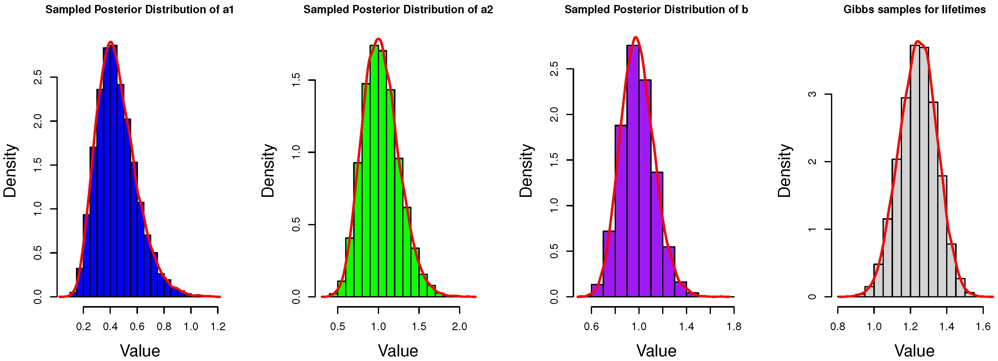
In addition, to show the details of Gibbs sampler and obtain more information of the posterior distributions, we present the histograms of Gibbs samples for unknown parameters and the estimated lifetimes of the censored data. Due to space limitations, only part of the results are presented here in Figure 6, Figure 7 and Figure 8.

Figure 6. Histograms of Gibbs samples for parameters and censored lifetimes when n = 30 and $(\alpha ,\beta )=(0.5,0.5)$.

Figure 7. Histograms of Gibbs samples for parameters and censored lifetimes when n = 50 and $(\alpha ,\beta )=(0.5,0.5)$.

Figure 8. Histograms of Gibbs samples for parameters and censored lifetimes when n = 100 and $(\alpha ,\beta )=(0.5,0.5)$.

Table 2, Table 3 and Table 4 show the results of the point estimators, including the MLEs and Bayesian estimators for $a_1$, $a_2$, and b, where `$OPT$’ and `$EM$’, respectively, refer to the MLE results obtained by the optim function and the EM algorithm. And prior 1 refers to the non-informative prior, while prior 2 refers to the informative prior. In addition, pc refers to the censoring proportion under the corresponding scheme and ‘$BE$’ refers to the Bayesian estimator. We discuss different censoring schemes by setting different values of the parameters $\alpha$ and $\beta$.

Table 2. Biases and MSEs corresponding to different estimates for $a_1$.

$(\mathit{\alpha },\mathit{\beta })$	pc	n		MLE		BE
				OPT	EM	Prior 1	Prior 2
(0.5, 0.5)	0.19	30	bias	0.0241	0.0241	−0.0503	0.0099
			mse	0.0328	0.0330	0.0348	0.0282
		50	bias	0.0101	0.0100	−0.0510	0.0010
			mse	0.0166	0.0166	0.0310	0.0174
		100	bias	0.0078	0.0077	−0.0524	−0.0049
			mse	0.0077	0.0077	0.0265	0.0071
(0.5, 1)	0.14	30	bias	0.0188	0.0186	−0.0421	0.0019
			mse	0.0309	0.0311	0.0362	0.0246
		50	bias	0.0102	0.0101	−0.0501	0.0016
			mse	0.0165	0.0165	0.0332	0.0154
		100	bias	0.0074	0.0073	−0.0640	−0.0011
			mse	0.0077	0.0077	0.0361	0.0076
(1, 0.5)	0.28	30	bias	0.0195	0.0195	−0.0553	−0.0036
			mse	0.0318	0.0318	0.0399	0.0253
		50	bias	0.0104	0.0103	−0.0509	−0.0098
			mse	0.0169	0.0169	0.0317	0.0148
		100	bias	0.0081	0.0080	−0.0784	−0.0111
			mse	0.0078	0.0078	0.0382	0.0076

Table 3. Biases and MSEs corresponding to different estimates for $a_2$.

($\mathit{\alpha },\mathit{\beta }$)	pc	n		MLE		BE
				OPT	EM	Prior 1	Prior 2
(0.5, 0.5)	0.19	30	bias	0.0249	0.0249	−0.0860	0.0123
			mse	0.0617	0.0622	0.0993	0.0542
		50	bias	0.0182	0.0182	−0.0969	−0.0024
			mse	0.0361	0.0361	0.1002	0.0352
		100	bias	0.0139	0.0138	−0.0994	−0.0061
			mse	0.0156	0.0156	0.0936	0.0164
(0.5, 1)	0.14	30	bias	0.0270	0.0267	−0.0829	0.0066
			mse	0.0636	0.0641	0.1024	0.0537
		50	bias	0.0183	0.0182	−0.0963	0.0011
			mse	0.0354	0.0355	0.1008	0.0322
		100	bias	0.0132	0.0129	−0.1296	−0.0044
			mse	0.0153	0.0153	0.1324	0.0169
(1, 0.5)	0.28	30	bias	0.0275	0.0275	−0.1150	0.0015
			mse	0.0636	0.0636	0.1078	0.0593
		50	bias	0.0188	0.0185	−0.1198	−0.0171
			mse	0.0369	0.0368	0.1016	0.0313
		100	bias	0.0145	0.0143	−0.1562	−0.0203
			mse	0.0156	0.0155	0.1372	0.0182

Table 4. Biases and MSEs corresponding to different estimates for b.

($\mathit{\alpha },\mathit{\beta }$)	pc	n		MLE		BE
				OPT	EM	Prior 1	Prior 2
(0.5, 0.5)	0.19	30	bias	0.0437	0.0440	0.0145	0.0756
			mse	0.0294	0.0296	0.0819	0.0362
		50	bias	0.0265	0.0267	-0.0195	0.0460
			mse	0.0163	0.0164	0.0892	0.0236
		100	bias	0.0111	0.0117	-0.0476	0.0324
			mse	0.0072	0.0073	0.0879	0.0090
(0.5, 1)	0.14	30	bias	0.0407	0.0420	-0.0032	0.0622
			mse	0.0288	0.0290	0.0866	0.0364
		50	bias	0.0267	0.0268	-0.0342	0.0433
			mse	0.0161	0.0159	0.0925	0.0212
		100	bias	0.0105	0.0115	-0.0916	0.0243
			mse	0.0071	0.0073	0.1259	0.0101
(1, 0.5)	0.28	30	bias	0.0436	0.0436	0.0365	0.0942
			mse	0.0305	0.0305	0.1037	0.0477
		50	bias	0.0282	0.0280	-0.0017	0.0818
			mse	0.0168	0.0168	0.0937	0.0281
		100	bias	0.0111	0.0111	-0.0735	0.0618
			mse	0.0072	0.0072	0.1349	0.0157

According to Table 2, Table 3 and Table 4 several conclusions are drawn as follows:

(1) Under different values of $(\alpha ,\beta )$, which represent different censoring schemes, the biases and MSEs of each estimator are very similar. This fully demonstrates that the model is robust to middle-censored data.

(2) As anticipated, for every estimator, both the bias and the MSE decline as the sample size n becomes larger. This indicates an improvement in their performance.

(3) When it comes to the results of MLE of each parameter, the performance of the two methods, namely the optimization method and the EM algorithm, is quite similar.

(4) In the situation where the sample size n is limited (e.g., $n=30$), Bayesian estimators exhibit lower MSEs compared to MLEs, which indicates that, in small-sample scenarios, the Bayesian method outperforms the classical frequentist method.

(5) As expected, the Bayesian estimators under informative prior distribution perform better than those under non-informative prior distribution.

Table 5, Table 6 and Table 7 present the results of interval estimates of $a_1$, $a_2$, and b, where ‘CP’ refers to the coverage percentages and ‘AW’ refers to the average widths of interval estimates. ‘HPD-P1’ and ‘HPD-P2’ represent the HPD credible intervals under non-informative and informative prior distribution, respectively.

Table 5. Average width and coverage percentage for interval estimation of $a_1$ when $\gamma$ = 0.05.

($\mathit{\alpha },\mathit{\beta }$)	pc	n	ACI		HPD-P1		HPD-P2
			AW	CP	AW	CP	AW	CP
(0.5, 0.5)	0.19	30	0.6490	0.9280	0.5367	0.8540	0.5914	0.9170
		50	0.4938	0.9500	0.4204	0.8600	0.4610	0.9090
		100	0.3480	0.9460	0.2993	0.8540	0.3288	0.9430
(0.5, 1)	0.14	30	0.6420	0.9220	0.5425	0.8610	0.5845	0.9290
		50	0.4920	0.9530	0.4208	0.8500	0.4611	0.9320
		100	0.3466	0.9430	0.2905	0.8280	0.3299	0.9410
(1, 0.5)	0.28	30	0.6495	0.9310	0.5273	0.8410	0.5781	0.9010
		50	0.4966	0.9500	0.4174	0.8420	0.4521	0.9300
		100	0.3498	0.9470	0.2823	0.7850	0.3242	0.9310

Table 6. Average width and coverage percentage for interval estimation of $a_2$ when $\gamma$ = 0.05.

($\mathit{\alpha },\mathit{\beta }$)	pc	n	ACI		HPD-P1		HPD-P2
			AW	CP	AW	CP	AW	CP
(0.5, 0.5)	0.19	30	0.9264	0.9380	0.7919	0.8640	0.8571	0.9390
		50	0.7095	0.9410	0.6088	0.8520	0.6638	0.9350
		100	0.4987	0.9500	0.4309	0.8550	0.4719	0.9200
(0.5, 1)	0.14	30	0.9191	0.9370	0.7939	0.8800	0.8519	0.9320
		50	0.7044	0.9420	0.6082	0.8730	0.6656	0.9300
		100	0.4951	0.9530	0.4166	0.8210	0.4729	0.9400
(1, 0.5)	0.28	30	0.9374	0.9460	0.7697	0.8500	0.8484	0.9100
		50	0.7170	0.9400	0.5983	0.8360	0.6563	0.9320
		100	0.5035	0.9580	0.4046	0.8020	0.4671	0.9210

Table 7. Average width and coverage percentage for interval estimation of b when $\gamma$ = 0.05.

($\mathit{\alpha },\mathit{\beta }$)	pc	n	ACI		HPD-P1		HPD-P2
			AW	CP	AW	CP	AW	CP
(0.5, 0.5)	0.19	30	0.6830	0.9550	0.5951	0.9050	0.6172	0.9410
		50	0.5181	0.9610	0.4467	0.8630	0.4705	0.9240
		100	0.3592	0.9510	0.3064	0.8600	0.3296	0.9410
(0.5, 1)	0.14	30	0.6621	0.9430	0.5839	0.8920	0.6111	0.9430
		50	0.5043	0.9550	0.4386	0.8740	0.4685	0.9260
		100	0.3497	0.9660	0.2916	0.8240	0.3269	0.9460
(1, 0.5)	0.28	30	0.7239	0.9760	0.6167	0.8630	0.6341	0.9140
		50	0.5486	0.9820	0.4585	0.8450	0.4906	0.9040
		100	0.3783	0.9790	0.3003	0.7860	0.3416	0.8880

Through Table 5, Table 6 and Table 7, we can observe that:

(1) Similarly to point estimations, the influence of different censoring schemes on the performance of interval estimators is relatively small.

(2) As the sample size n grows, confidence interval widths decrease, and coverage percentages generally rise.

(3) Bayesian interval estimates under informative prior perform better than those under non-informative prior.

5.2. Real Data Analysis

We apply real-world data from [9] in this subsection to demonstrate the inference framework developed in this study.

The real dataset is from the National Eye Institute diabetic retinopathy study, whose purpose is to examine the influence of laser treatment on the delay of the start of blindness in those suffering from diabetic retinopathy. With respect to the i-th participant, $X_{i,1}$ represents the blind time of the eye which has received laser treatment, while $X_{i,2}$ refers to the blind time of the untreated eye. Then, the time of first onset of blindness $T_i=min\{X_{i,1},X_{i,2}\}$. Therefore, this dataset exhibits characteristics of competing risks data. Original data with corresponding cause are in Table 8.

Table 8. The original data of the blind time with corresponding cause.

Unit: Days
(266, 1)	(583, 1)	(79, 1)	(93, 1)	(805, 1)	(344, 1)	(306, 1)	(415, 1)
(178, 1)	(1484, 1)	(315, 1)	(1252, 1)	(642, 1)	(407, 1)	(356, 1)	(699, 1)
(667, 1)	(126, 1)	(350, 1)	(84, 1)	(392, 1)	(901, 1)	(276, 1)	(520, 1)
(503, 1)	(584, 1)	(355, 1)	(1302, 1)	(91, 2)	(154, 2)	(547, 2)	(707, 2)
(469, 2)	(1313, 2)	(790, 2)	(125, 2)	(777, 2)	(307, 2)	(637, 2)	(577, 2)
(517, 2)	(287, 2)	(717, 2)	(141, 2)	(427, 2)	(36, 2)	(588, 2)	(350, 2)
(567, 2)	(1140, 2)	(448, 2)	(904, 2)	(485, 2)	(248, 2)	(423, 2)	(285, 2)
(315, 2)	(727, 2)	(210, 2)	(409, 2)	(227, 2)

To ensure that the solution exists, we divide the data by 365 to let the unit be year. It should be noted that, before further analysis, we need to first determine whether the dataset is able to be analyzed using the Burr-XII distribution. Separately for failure cause 1 and 2, initially, the complete dataset is employed to derive MLEs of unknown parameters, followed by the application of the Kolmogorov–Smirnov test. For cause 1, the MLEs of $a_1$ and $b_1$ are 0.9033 and 2.3703, respectively. The value of Kolmogorov–Smirnov statistics is 0.1168 with its corresponding p-value $=0.7978$. For cause 2, the MLEs of $a_2$ and $b_2$ are 0.9237 and 2.4605, respectively. The value of Kolmogorov–Smirnov statistics equals 0.1470 with its corresponding p-value amounting to 0.4324. Consequently, we can conclude that the Burr-XII distribution can be used to fit the dataset mentioned above.

In addition, $b_1=b_2=b$ need to be tested. We use the likelihood ratio test method. Through the analysis and calculation of the sample data, the corresponding p-value is quite close to 1, which indicates that the hypothesis “$b_1=b_2=b$” is reasonable.

Then, we generate the artificial data. Both the left endpoint and the interval length are the random variables which follow the exponential distribution with mean 1. The processed data (measured in years) are presented in Table 9.

Table 9. The artificial middle-censored data.

Cause	Data (Years)
Cause 1	0.7288	0.2164	0.2548	2.2055
	0.9425	1.1370	4.0658	1.0740
	0.8630	3.4301	1.7589	1.1151
	1.9151	1.8274	0.9589	0.2301
	0.9726	3.5671	0.7562	1.4247
	1.6000	[0.0911, 5.0378]	[0.6011, 1.7187]	[0.3192, 0.6168]
	[0.8229, 1.0968]	[0.0267, 0.5380]	[2.0658, 4.4214]	[0.1413, 2.1862]
Cause 2	0.2493	1.4986	1.9370	1.2849
	3.5973	2.1644	0.3425	2.1288
	1.7452	1.5808	1.9644	0.3863
	1.1699	0.0986	1.5534	1.2274
	2.4767	1.1589	0.7808	0.8630
	1.9918	0.5753	1.1205	0.6219
	[0.1226, 0.9680]	[0.6727, 2.0312]	[0.4918, 2.2852]	[0.4439, 0.9947]
	[0.7571, 2.0435]	[0.0610, 1.6743]	[0.9411, 3.4598]	[0.3921, 1.3314]
	[0.1619, 1.0728]

Since we have no extra information of $a_1,$$a_2$, and b, we employ the non-informative priors for them.

Using the methods and procedures of estimation outlined above, point and interval estimates for all unknown parameters are derived, with results shown in Table 10, where ‘$ML{E}_{OPT}$’, ‘$ML{E}_{EM}$’ represent the MLEs obtained by the optim function or the EM algorithm, respectively, and ‘BE’ refers to the Bayesian point estimator. We can see that the results from two methods to obtain MLEs are same and the widths of HPDs are less than those of ACIs.

Table 10. The result of different point and interval estimates for $a_1,a_2,b$.

	${\mathit{MLE}}_{\mathit{OPT}}$	${\mathit{MLE}}_{\mathit{EM}}$	BE	ACI	HPD
$a_1$	0.4339	0.4339	0.3025	[0.2584, 0.6095]	[0.1832, 0.4357]
$a_2$	0.5114	0.5114	0.3571	[0.3182, 0.7047]	[0.1664, 0.4951]
b	2.3292	2.3292	2.0231	[1.6961, 2.9624]	[1.5444, 2.5151]

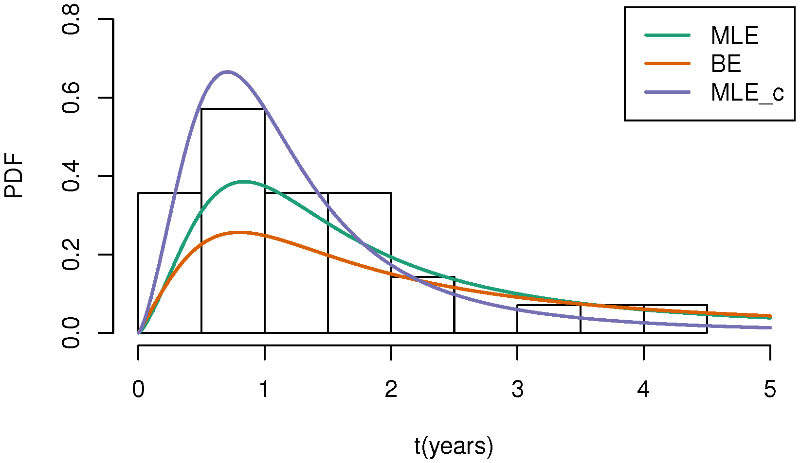
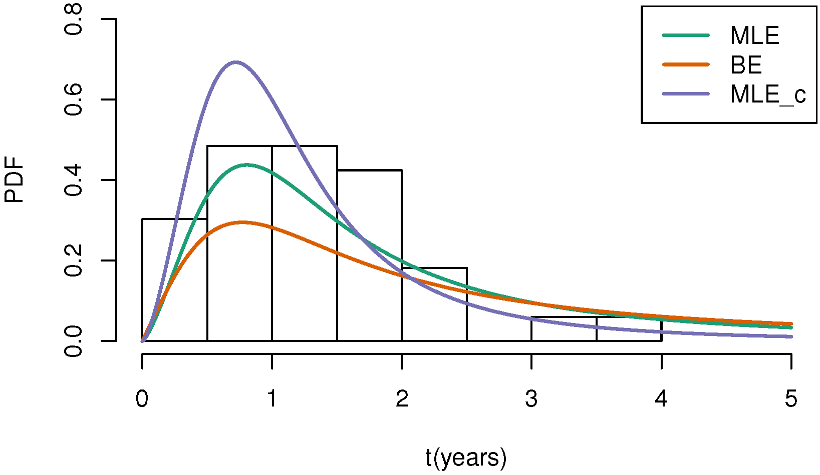
Based on the estimated values of parameters $a_1,a_2$, and b, we can draw plots that combine the fitted probability density curves with the frequency histograms of the complete data for the two causes, respectively.

In Figure 9 and Figure 10, ‘MLE’ denotes the density curve based on MLEs under middle-censored data, ‘BE’ denotes the curve based on Bayes estimates under middle-censored data, and ‘MLE_c’ represents the density curve with parameter estimates derived from the complete data. Through Figure 9 and Figure 10, we can conclude that the estimated density curve is generally consistent with the trend of the frequency distribution of the real dataset, and its peak point is close to the peak point of the real dataset, indicating that our model is valuable in practical application.

Figure 9. The fitted PDF plots for sample data corresponding to cause 1.

Figure 10. The fitted PDF plots for sample data corresponding to cause 2.

6. Conclusions

This study mainly concentrates on statistical analysis for the middle-censored data with Burr XII distribution under independent competing risk frameworks. We apply both frequentist and Bayesian approaches to derive parameter estimates.

In the frequentist approach, we present the maximum likelihood estimates and prove their existence and uniqueness. Applying the observed Fisher information matrix, we calculate the ACIs.

Regarding Bayesian estimation, we utilize adaptive rejection sampling and Gibbs sampling techniques. These are employed to compute the Bayesian estimates under the squared error loss function, along with the corresponding HPD credible intervals.

Moreover, a simulation is performed with the aim of observing the performance of various estimations. After comparison, we find that for small-size samples, the Bayesian estimation with prior information performs better. The interval estimate obtained using the Bayesian method has a shorter width. At last, we apply our model to analyze an authentic dataset related to medicine, confirming that our model is reasonable.

Although the current study provides valuable information on the estimation issues regarding the middle-censored data combined with the independent competing risks, there are several areas for future improvement and exploration. One possible direction is to extend the analysis by considering that the value of b for the Burr-XII distribution of each failure cause may vary. Another important aspect for future research is the consideration of dependent competing risks. Within this study, we focus on the basic assumption of independent competitive risks, but in real-world scenarios, the risks may not always be independent. Exploring the implications of dependent competing risks would offer a more comprehensive analysis under complex conditions.

References

1. Jammalamadaka, S.R.; Mangalam, V. Nonparametric estimation for middle-censored data. J. Nonparametr. Stat. 2003, 15, 253–265. [Google Scholar] [CrossRef]
2. Jammalamadaka, S.R.; Iyer, S.K. Approximate self consistency for middle-censored data. J. Stat. Plan. Inference 2004, 124, 75–86. [Google Scholar] [CrossRef]
3. Iyer, S.K.; Jammalamadaka, S.R.; Kundu, D. Analysis of middle-censored data with exponential lifetime distributions. J. Stat. Plan. Inference 2008, 138, 3550–3560. [Google Scholar] [CrossRef][Green Version]
4. Davarzani, N.; Parsian, A. Statistical inference for discrete middle-censored data. J. Stat. Plan. Inference 2011, 141, 1455–1462. [Google Scholar] [CrossRef]
5. Jammalamadaka, S.R.; Bapat, S.R. Middle censoring in the multinomial distribution with applications. Stat. Probab. Lett. 2020, 167, 108916. [Google Scholar] [CrossRef]
6. Abuzaid, A.H.; El-Qumsan, M.K.A.; El-Habil, A.M. On the robustness of right and middle censoring schemes in parametric survival models. Commun. Stat. Simul. Comput. 2015, 46, 1771–1780. [Google Scholar] [CrossRef]
7. Wang, L. Estimation for exponential distribution based on competing risk middle censored data. Commun. Stat. Theory Methods 2016, 45, 2378–2391. [Google Scholar] [CrossRef]
8. Ahmadi, K.; Rezaei, M.; Yousefzadeh, F. Statistical analysis of middle censored competing risks data with exponential distribution. J. Stat. Comput. Simul. 2017, 87, 3082–3110. [Google Scholar] [CrossRef]
9. Wang, Y.; Shi, Y.; Wu, M. Statistical inference for dependence competing risks model under middle censoring. J. Syst. Eng. Electron. 2019, 30, 209–222. [Google Scholar]
10. Davarzani, N.; Parsian, A.; Peeters, R. Statistical Inference on Middle-Censored Data in a Dependent Setup. J. Stat. Res. 2014, 9, 646–657. [Google Scholar] [CrossRef]
11. Sankaran, P.G.; Prasad, S. Weibull Regression Model for Analysis of Middle-Censored Lifetime Data. J. Stat. Manag. Syst. 2014, 17, 433–443. [Google Scholar] [CrossRef]
12. Rehman, H.; Chandra, N. Inferences on cumulative incidence function for middle censored survival data with Weibull regression. J. Appl. Stat. 2022, 5, 65–86. [Google Scholar] [CrossRef]
13. Sankaran, P.G.; Prasad, S. Additive risks regression model for middle censored exponentiated-exponential lifetime data. Commun. Stat. Simul. Comput. 2018, 47, 1963–1974. [Google Scholar] [CrossRef]
14. Zimmer, W.J.; Keats, J.B.; Wang, F.K. The Burr XII Distribution in Reliability Analysis. J. Qual. Technol. 1998, 30, 386–394. [Google Scholar] [CrossRef]
15. Soliman, A.A. Estimation of Parameters of Life from Progressively Censored Data Using Burr-XII Model. IEEE Trans. Reliab. 2005, 54, 34–42. [Google Scholar] [CrossRef]
16. Yan, W.; Li, P.; Yu, Y. Statistical inference for the reliability of Burr-XII distribution under improved adaptive Type-II progressive censoring. Appl. Math. Model. 2021, 95, 38–52. [Google Scholar] [CrossRef]
17. Du, Y.; Gui, W. Statistical inference of Burr-XII distribution under adaptive type II progressive censored schemes with competing risks. Results Math. 2022, 77, 81. [Google Scholar] [CrossRef]
18. Abuzaid, A.H. The estimation of the Burr-XII parameters with middle-censored data. J. Appl. Probab. Stat. 2015, 4, 101. [Google Scholar] [CrossRef][Green Version]
19. Cox, D.R. The analysis of exponentially distributed life - times with two types of failure. J. R. Stat. Soc. Ser. B Stat. Methodol. 1959, 21, 411–421. [Google Scholar] [CrossRef]
20. Qin, X.; Gui, W. Statistical inference of Burr-XII distribution under progressive Type-II censored competing risks data with binomial removals. J. Comput. Appl. Math. 2020, 378, 112922. [Google Scholar] [CrossRef]
21. Chacko, M.; Mohan, R. Bayesian analysis of Weibull distribution based on progressive type-II censored competing risks data with binomial removals. Comput. Stat. 2018, 34, 233–252. [Google Scholar] [CrossRef]
22. Dempster, A.P.; Laird, N.M.; Rubin, D.B. Maximum likelihood from incomplete data via the EM algorithm. J. R. Stat. Soc. Ser. B 1977, 39, 1–22. [Google Scholar] [CrossRef]
23. Fisher, R.A. On the mathematical foundations of theoretical statistics. Philos. Trans. R. Soc. Lond. Ser. A Contain. Pap. A Math. Phys. Character 1922, 222, 309–368. [Google Scholar]
24. Gilks, W.R.; Wild, P. Adaptive Rejection Sampling for Gibbs Sampling. Appl. Stat. 1992, 41, 337–348. [Google Scholar] [CrossRef]
25. Chen, M.-H.; Shao, Q.-M. Monte Carlo Estimation of Bayesian Credible and HPD Intervals. J. Comput. Graph. Stat. 1999, 8, 69–92. [Google Scholar] [CrossRef]
Disclaimer/Publisher’s Note: The statements, opinions and data contained in all publications are solely those of the individual author(s) and contributor(s) and not of MDPI and/or the editor(s). MDPI and/or the editor(s) disclaim responsibility for any injury to people or property resulting from any ideas, methods, instructions or products referred to in the content.
Article Metrics
Citations
Article Access Statistics
Multiple requests from the same IP address are counted as one view.