Evolutionary Approach to the Euclidean Steiner Tree Problem in n-Space

Abstract

This article presents the application of a genetic algorithm for solving the Euclidean Steiner problem in spaces of dimensionality greater than 2. The Euclidean Steiner problem involves finding the minimum spanning network that connects a given set of vertices, including the additional Steiner vertices, in a multi-dimensional space. The focus of this research is to compare several different settings of the method, including the crossover operators and sorting of the input data. The paper points out that significant improvement in results can be achieved through proper initialization of the initial population, which depends on the appropriate sorting of vertices. Two approaches were proposed, one based on the nearest neighbor method, and the other on the construction of a minimum spanning tree.

1. Introduction

The Euclidean Steiner Tree Problem (ESTP) in ${\mathbb{R}}^n$ concerns finding the minimal network of connections for a set of points P. This network forms a tree structure, where the length of the network is the sum of the lengths of edges connecting the vertices. If no additional points can be used to connect the points in P, the problem reduces to finding a minimum spanning tree (MST) for P, which can be efficiently solved using algorithms such as Prim’s algorithm. However, if it is possible to add additional intermediate points, known as Steiner points, networks of shorter length (Steiner Minimal Tree, SMT) can be obtained. This, however, is a significantly more complex problem as both the number and the location of the additional Steiner points are unknown. It has been proven to be an NP-hard problem in both 2D Euclidean space and in higher-dimensional spaces.

Figure 1 shows an example of a minimal spanning tree and a minimal Steiner tree for ten points in 2D space (${\mathbb{R}}^2$). A similar example is presented in Figure 2 for ten points in 3D space (${\mathbb{R}}^3$). In both cases, the total length of edges is smaller for SMT compared to MST.

Figure 1. An example of a minimal spanning tree (left) and a minimal Steiner tree (right) in 2D. Additional Steiner points are presented as squared marks.

Figure 2. An example of a minimal spanning tree (left) and a minimal Steiner tree (right) in 3D. Additional Steiner points are presented as squared marks.

ESTP in 2D Euclidean space ${\mathbb{R}}^2$ is particularly noteworthy because there exist efficient algorithms that can solve problems for $p=\left|P\right|$ on the order of thousands. An example of such an algorithm is the GeoSteiner algorithm. However, efficient algorithms in 2D are based on characteristics of the Steiner problem specific to the plane and cannot be utilized to develop equally efficient algorithms in 3D space or in higher-dimensional spaces.

The aim of this study is to exploit the potential of the genetic algorithm to build a search algorithm for exploring the space of possible full Steiner topologies (FST) and then to evaluate the so-called relative minimal trees (RMT), which can be obtained from them through the optimization of the Steiner points’ positions. Among the evaluated RMTs, the one with the smallest sum of edges is selected as the SMT. All necessary definitions and characteristics of the used structures will be described in the following sections. The proposed algorithm will be tested on a set of problems in 3D space with sizes $p=17$ and $p=100$.

1.1. Definitions

The following definitions and characteristics of ESTP will be used in this paper. They are correct for the Euclidean space ${\mathbb{R}}^n$ for any n.

Points in P are called terminals, and it is assumed that their count is p. Points in S are Steiner points. For an optimal solution to the ESTP of size p, the maximum number of Steiner points in the SMT (Steiner Minimum Tree) is $p-2$. The degree conditions are also met: (1) in the SMT, a terminal from P can only have a degree of 1, 2, or 3; (2) a Steiner point in the SMT has a degree exactly equal to 3. The angle condition can be formulated as follows: Every Steiner point and the three points it is connected to lie on a plane, and the edges connecting the vertices form angles of 120 degrees. A tree that meets the angle condition is called a Steiner tree.

If we fix the number of Steiner points and the way they are connected to vertices from P but do not determine the location of the Steiner points, we define the Steiner topology. If in a given topology we use the maximum number of Steiner points, which is $p-2$, then such a topology is called a full Steiner topology (FST). Such a full topology describes a Steiner tree in which each terminal has a degree equal to 1.

As mentioned, for a given FST (Full Steiner Topology), the positions of the Steiner points are not determined. If these positions are optimized in such a way that the resulting tree has the minimum total edge length, a so-called relatively minimal tree (RMT) for the given topology is formed. If during the optimization process of the Steiner points’ positions their locations coincide with terminal points or other Steiner points, then the obtained RMT is referred to as a degeneration of the given topology. An RMT for a given topology always exists. A very important feature of the problem under consideration is the fact that for an SMT (Steiner Minimum Tree) in a given ESTP (Euclidean Steiner Tree Problem), there always exists an FST whose RMT is equal to the given MST.

From the above description, a general approach to the ESTP emerges: for a given set P, construct successive FSTs, find their RMTs, and present the smallest of them as the SMT (Steiner Minimum Tree). Many exact algorithms approach the ESTP in this way, trying to limit the number of FSTs checked. A review of these methods can be found in [1]. In this paper, a different approach is proposed. Instead of developing methods to limit the number of FSTs checked, it is assumed that not all of them will be examined. Instead, a genetic algorithm is used to optimize successive FSTs. This is significant, as the space of possible FSTs grows rapidly for successive p.

Figure 3 shows an example of an FST for $p=5$. It is noted that the coordinates of the vertices are not important here, and only their mutual connections matter. This implies that in constructing an FST, the order in which terminals are added to the FST through a Steiner point is crucial. This fact will be utilized in the proposed approach based on the genetic algorithm. On the other hand, Figure 4 provides more details regarding the process of building an FST. Even if the order in which terminals are added to the FST is fixed, it is still possible to construct many different topologies by choosing how the new terminal is connected through a new Steiner point. For three terminals, there is only one unique way to connect them using one Steiner point. Figure 4 further shows that the fourth terminal can be added to the developing FST in three different ways through a new Steiner point. Starting from the initial three edges, adding each subsequent Steiner point and terminal increases the number of edges by 2. Therefore, adding the fifth vertex would be possible in five ways. Generally, adding the k-th Steiner point is possible in $2(k-1)+1$ ways, for $k=1,2,\dots ,p-2$, assuming the first Steiner point connects three terminals.

Figure 3. An example of a full Steiner topology (top) and its degeneracy (bottom) for five terminals $t_1-t_5$ (gray circles). Additional Steiner points are $s_1,s_2$ and $s_3$ (white circles).

Figure 4. Construction of full Steiner topologies (terminal points presented as gray and Steiner points as white circles). Top: a unique full Steiner topology for three terminals $t_1-t_3$ with just one Steiner point $s_1$. Bottom: three full Steiner topologies for four terminals $t_1-t_4$. The new terminal $t_4$ is attached through a new Steiner point $s_2$, which is connected to edge 1 (left), edge 2 (middle), or edge 3 (right).

The number of possible full topologies increases very rapidly with p and is given by the following formula:

$$2^{-(p-2)}{\displaystyle \frac{(2p-4)!}{(p-2)!}}$$

This reflects the combinatorial complexity of the problem, illustrating how the space of potential solutions expands with each additional terminal. Starting from $p=12$, this value is greater than $p!$ (654,729,075 vs. 479,001,600).

1.2. Related Work

The Steiner Minimal Tree problem has diverse applications in several technological and scientific domains. One of the primary applications of the Steiner Tree Problem is in network design, where it helps in minimizing the total length of networks, such as telecommunications and computer networks. This has practical implications for reducing costs and increasing the efficiency of network infrastructure. [2] provides a comprehensive overview of the SMT problem in various contexts, including network design. In the realm of electronics, the SMT Problem is crucial for optimizing the layout of circuits in VLSI (Very Large-Scale Integration) designs [3]. The objective is to minimize the total wire length, which is critical for enhancing the performance and reducing the power consumption. In biology, the SMT is used in phylogenetics to infer the shortest evolutionary tree. This application involves finding the most parsimonious tree connecting different species based on genetic markers [4]. Robotics applications can use Steiner trees for path planning, especially in the context of navigating complex environments where paths need to be as efficient as possible. A good overview of industrial applications of the Steiner problem is provided in [5]. The Steiner problem formulation also appears in other optimization problems that can be termed hybrid, such as the Steiner Traveling Salesman Problem in [6].

For the ESTP in two dimensions, an exact and efficient algorithm was proposed by [7]. The GeoSteiner program [8] is a successful implementation of this algorithm, which was based on the efficient enumeration of all topologies. However, the methods used in this two-dimensional approach cannot be directly translated to higher dimensions. In [9], a solution to the ESTP in ${\mathbb{R}}^d$ for $d\ge 3$ was proposed through the enumeration of all topologies, yet this approach is inefficient. One of the most important approaches to solving the ESTP accurately in ${\mathbb{R}}^d$ is the branch and bound method presented by Smith in [10]. However, the practical usefulness of this method largely depends on how well the lower bound can be estimated at the nodes of the search tree. Other studies have tried to introduce improvements to Smith’s algorithm, for example, [11]. However, the results presented in this study were for problems with 18 terminal points and thus relatively small-scale problems. Another work proposing improvements to Smith’s algorithm is [12]. In [13], the ESTP in ${\mathbb{R}}^d$ was formulated as a convex mixed-integer nonlinear programming (MINLP), and results were presented for problems with 10 terminal points. A good overview of algorithms for finding exact solutions to the ESTP is provided in [1]. An excellent and up-to-date introduction to the issues related to the Euclidean Steiner problem and the challenges in higher-dimensional spaces is presented in [14].

The Iterated Local Search algorithm was proposed in [15] as an example of a heuristic approach. The genetic algorithm has been applied to the ESTP in two-dimensional space, as demonstrated in [16,17,18,19]. Other evolutionary algorithms, such as memetic algorithms, have also been developed for ${\mathbb{R}}^2$ [20]. Another example is an application of particle swarm optimization algorithm to optimize the network connecting cities in China [21]. Additional heuristics, like Monte Carlo Tree Search, were also explored in [22]. The genetic algorithm has also been utilized in other variations of the Steiner problem, for instance, [23] for the rectilinear Steiner tree problem, and for the Prize-Collecting Steiner Tree Problem [24]. However, the application of the genetic algorithm to the ESTP in ${\mathbb{R}}^d$ for $d\ge 3$ remains unexplored. This publication aims to fill that gap. The aim of this publication is to present a new approach based on a genetic algorithm and to test the significance of various parameters of this approach. We do not aspire to provide an exhaustive review of other existing heuristics, such as [25], leaving a more comprehensive experimental comparison for future research.

1.3. The Contribution of This Work

This publication addresses a specific gap in the use of genetic algorithms for optimizing connection networks within Euclidean space. Specifically, it presents a tailored implementation of an evolutionary heuristic adapted to the Euclidean Steiner Tree Problem (ESTP) in ${\mathbb{R}}^d$ for $d\ge 3$. It demonstrates how to represent the problem as a discrete optimization issue. The impact of various factors on the quality of the solutions obtained was examined. It was noted that the proposed method for generating the initial population, based on a heuristic that utilizes sorting according to the order of vertex addition by the Prim algorithm constructing a minimum spanning tree, has a significant influence on the results. Different configurations of the algorithm were tested on sets of problems with 17 and 100 points. The results were subjected to a statistical significance analysis.

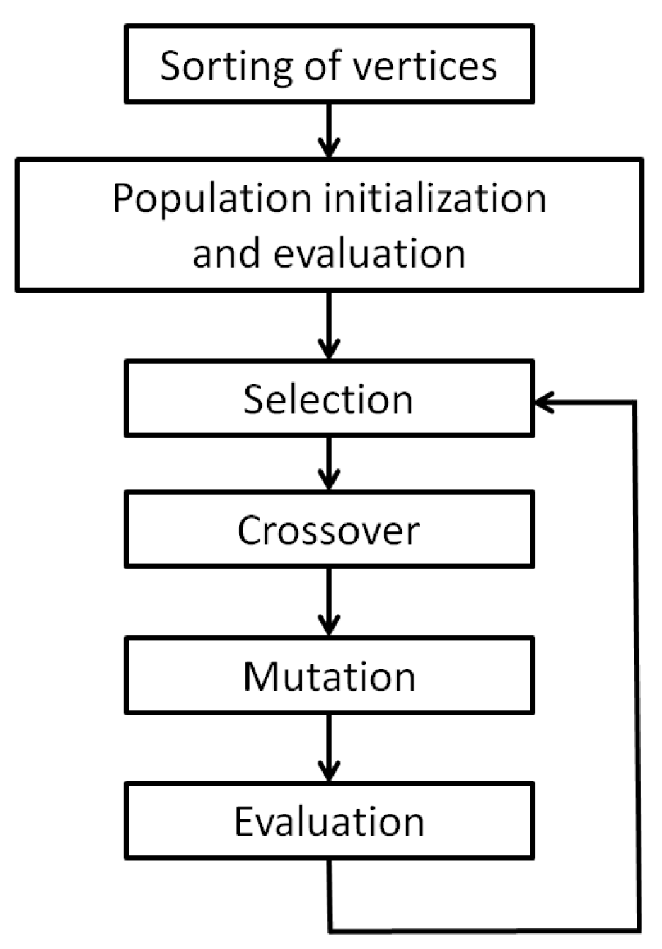
2. Proposed Algorithm

The proposed solution is based on a genetic algorithm. A genetic algorithm is a meta-heuristic often used in challenging optimization problems, including combinatorial ones. The general principle of operation is based on simulating the Darwinian process of natural selection by promoting better solutions from the current population. This selective pressure promotes more promising solutions, which, after undergoing the selection process, serve to generate new, potentially better solutions as a result of applying the appropriate operators. These operators typically include a crossover operator, which generates a new solution based on two selected ones, and a mutation operator, which creates a new solution by randomly altering an existing one. Repeatedly performing selection, crossover, and mutation steps (combined with a procedure for evaluating the quality of each new solution) has significant practical potential for locating areas in the search space with high-quality solutions. The genetic algorithm is a heuristic and, therefore, does not guarantee finding the optimal solution; however, in practice, it often provides satisfactory solutions within a reasonable time frame. The genetic algorithm can also be called a meta-heuristic, meaning it is a general approach to solving optimization problems and needs to be adapted to a specific problem. To carry this out, it is essential, first and foremost, to choose an appropriate data structure capable of representing a solution in the given optimization problem. The data structure should allow for some way of encoding the solution it represents. The chosen data structure also dictates the possible crossover and mutation operations. A schematic representation of the genetic algorithm is shown in Figure 5. In the following sections, we describe the individual steps and assumptions made to adapt the genetic algorithm to solving the ESTP in Euclidean space of any dimensionality.

Figure 5. General scheme of genetic algorithm.

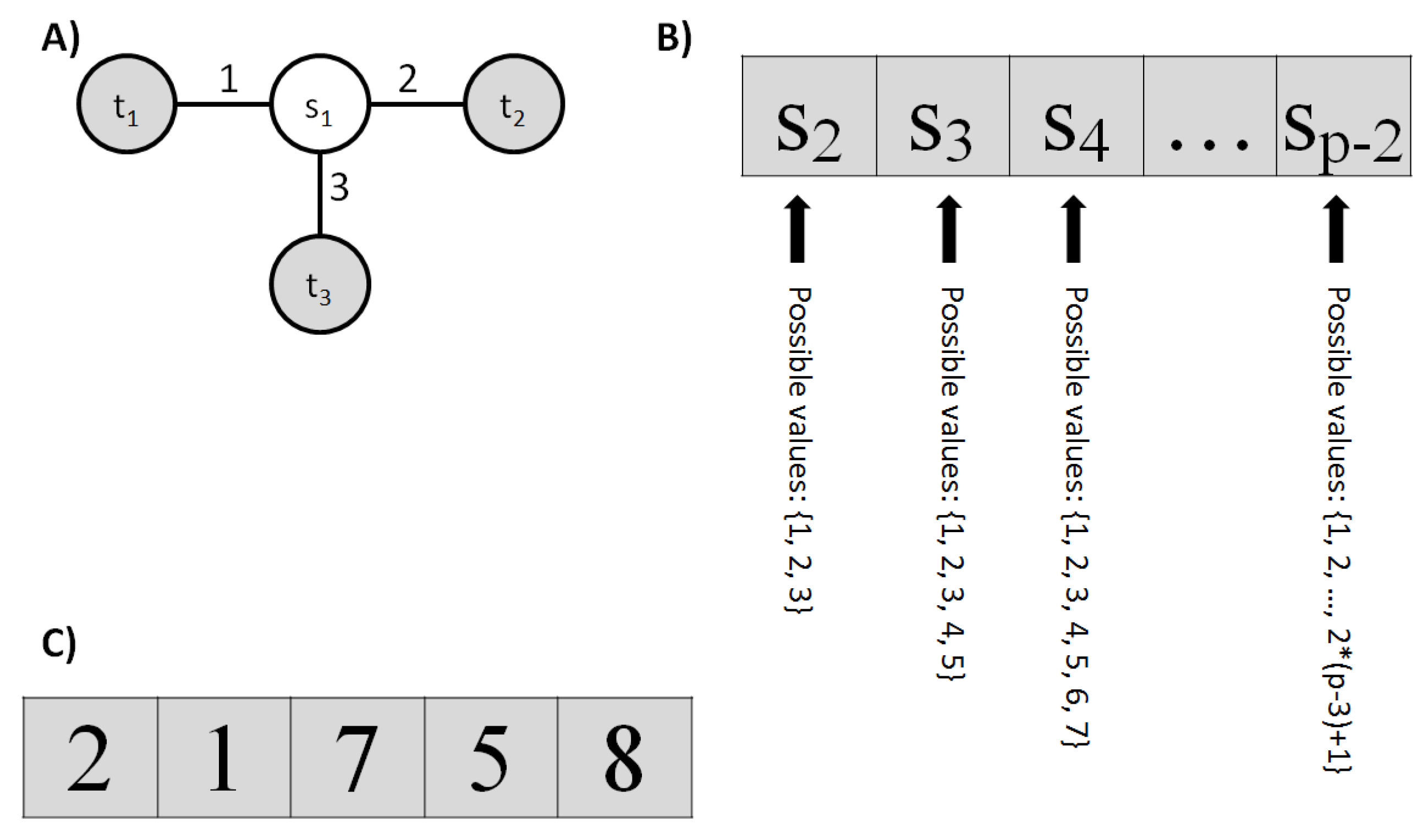
2.1. Data Structure

In the ESTP, it is necessary to determine both the number and coordinates of Steiner points. A naive approach to the ESTP would be to encode just these two pieces of information. However, this is not the best approach, as it does not utilize previous algorithmic achievements related to the ESTP, including the ability to efficiently calculate the RMT for a given FST. Such an algorithm was provided in [10], where he also proposed an efficient way of encoding information about a given FST. This method is very simple and simultaneously relates to the previously mentioned process of building an FST in the process of adding successive terminals through another Steiner point.

Here, we assume that the order of terminal attachment follows a certain adopted sequence, which is irrelevant at this point. The initiation of the FST construction begins by taking the first three terminals and connecting them with the first Steiner point. However, attaching the fourth terminal can occur in three ways, the fifth in five, the sixth in seven, generally in $2\ast (k-1)+1$ for $k=1,\dots ,p-2$. This leads to the proposed data structure as a vector of $p-3$ integers $fst=[s_2,s_3,\dots ,s_{p-2}]$, where the possible value for $s_k$ depends on its position, meaning $s_k$ belongs to the interval $[1,2\ast (k-1)+1]$. Note that there is no need to encode the unique way the first Steiner point $s_1$ is connected. During the random initialization of the initial population, values for each $s_k$ are generated randomly from the appropriate interval for it.

In Figure 6, the general data structure used as a chromosome is graphically presented, along with a sample chromosome for the problem involving eight terminal points.

Figure 6. Scheme of the data structure used as a chromosome. For p points (terminals), we generally have $p-2$ potential Steiner points, each of which can be connected to the topology being generated in a number of ways depending on its index. (A) The first Steiner point $s_1$ uniquely connects the first three terminal points. (B) Each subsequent Steiner point, from index 2 to $p-2$, can be added in an increasing number of ways equal to $2(k-1)+1$, where k is the index of the Steiner point $s_k$. (C) A sample chromosome for the problem with $p=8$ terminal points. Thus, the number of potential Steiner points is $p-2=6$. The first of these does not require encoding in the chromosome, so the chromosome length is 5. Each position in the chromosome displays a random value from the allowable range.

At this point, it is worth emphasizing that the proposed data structure is independent of the dimensionality of the Euclidean space in which the Steiner problem is being solved. Its length depends solely on the number of terminal points, and the possible values depend only on their indices. The dimensionality of the space does not affect the representation of the solution as a chromosome encoded using this data structure. It will, however, influence the method of calculating the Euclidean distance between points; i.e., higher-dimensional Euclidean space will be more computationally demanding.

It is worth noting that adopting such a data structure to represent the solution turns the problem into a combinatorial optimization problem.

2.2. Population Initialization

In describing the data structure used for encoding the solution, the aspect of the order in which terminals are connected, i.e., their permutations, was omitted. It was assumed that this order is random, and the next terminal is connected with an equal probability by any existing edge. Let us call this the default initialization method. However, a brief analysis of the characteristic features of the problem allows for the development of better initialization methods. Below, we propose two such methods.

Firstly, it is worth noting that in an optimal SMT solution, it is more likely that a given terminal will be connected to another terminal (directly or via a Steiner point) if it is closer rather than farther away, using Euclidean distance. From this observation, a simple heuristic can be proposed for generating complete topologies in the initial population of FSTs. This heuristic involves, for each subsequent terminal added to the FST under construction, first finding a certain number of its nearest neighbors among the terminals already included in the FST. From these nearest neighbors, one is randomly selected, and its edge is used to connect the new terminal. In this work, we test the number of nearest neighbors at 2, 3, 4, and 5.

The second proposed heuristic for generating initial FSTs utilizes the first but aims to rectify its shortcomings. It addresses the issue that if the order of terminals is still random, then the nearest neighbors of a given terminal, searched only among other terminals already included in the FST under construction, may not be its nearest neighbors when searched across the entire set P. Therefore, as a second heuristic, we propose pre-sorting all terminals in P according to the order of their selection during the execution of Prim’s algorithm, which finds the minimum spanning tree for points in P. This procedure starts from a random initial point. This ordering is further motivated by the fact that the minimum spanning tree is a solution to the problem of minimal connections in the absence of the possibility of using Steiner points.

The results of numerical experiments presented later in the paper indicate that the application of an appropriate initialization procedure is of great significance.

2.3. Individual Evaluation

The evaluation of a given individual in the solution population involves assessing the quality of the RMT for the FST encoded by this individual. To obtain the RMT, it is necessary to optimize the placement of Steiner points so that the sum of the edge lengths is minimized while the topology of connections remains unchanged. The solution to this problem has been known for years and was proposed by Smith in his work [10]. In this paper, we use exactly this algorithm to evaluate the given FST. As a solution to the ESTP, the genetic algorithm provides the best-found RMT in any generation.

2.4. Selection

The selection method used was tournament selection. It involves drawing a specified number of individuals from the population with equal probability. The tournament is won by the best individual, and the procedure is repeated the required number of times (population size).

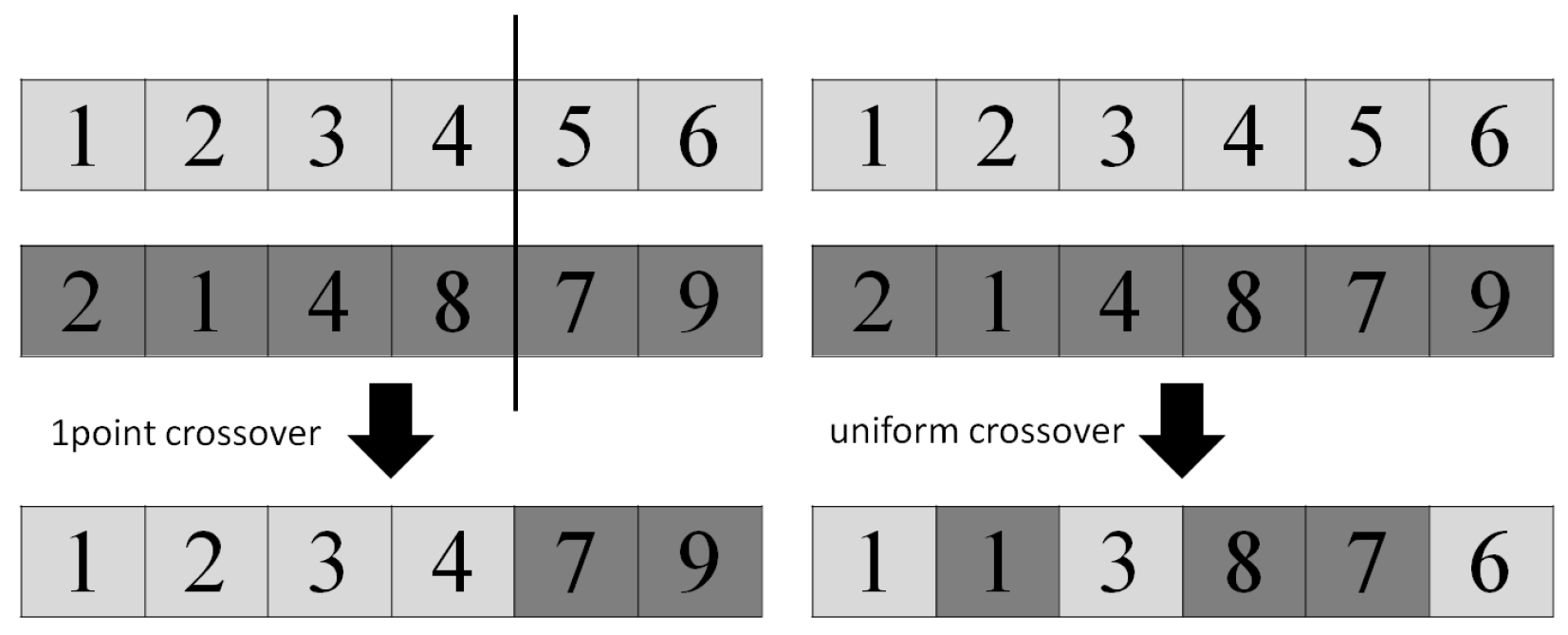
2.5. Crossover

In this paper, two crossover operators were compared: single-point and uniform. In single-point crossover, a single crossover point is randomly selected from two chromosomes (vectors of integers in our case). A new individual is created by cross-exchanging the corresponding parts between two solutions previously selected during the selection phase. It is also possible to create two offspring. In uniform crossover, each element of the new solution (offspring) is randomly chosen with equal probability from the two parental solutions. Figure 7 illustrates the schematic operation of both operators. It is important to note that both operators ensure that the new solution encodes a correct FST. The crossover itself occurs with a certain probability, which is a parameter of the genetic algorithm. If it does not occur, the original solution proceeds to the next step unchanged.

Figure 7. Example results of two crossover operators: 1-point crossover (left) and a uniform crossover (right).

2.6. Mutation

The mutation operator involves randomly selecting a new value for a specific position in the vector encoding the FST, with a certain probability. Depending on the position, the value is drawn from the appropriate range, the same one that was used in the random generation of the vector describing the FST. Therefore, an integer from the range $[1,2\ast (k-1)+1]$ is selected for the element $s_k$, where k ranges from 2 to $p-2$. This procedure also ensures the correctness of the resulting FST.

2.7. Computational Complexity

The proposed algorithm is based on an evolutionary algorithm, with its execution time directly dependent on the number of iterations of the main evolutionary loop. The primary computational cost of the proposed approach arises from the necessity of finding the RMT for a given FST encoded in the chromosome, which involves optimizing the positions of the Steiner points. Compared to this procedure, the computational costs of other operations, such as crossover and mutation, are negligible. Similarly, the use of the minimum spanning tree algorithm, applied only once during population initialization, has minimal impact. For p points, Prim’s algorithm has a worst-case complexity of $O\left(p^2\right)$, which can be reduced depending on the data structures used. Thus, the overall computational cost is approximately O(pop_size · iterations_num), where pop_size is the population size and iterations_num is the number of iterations of the main loop in the genetic algorithm. The complexity of the RMT optimization algorithm itself is detailed in [10].

2.8. Summary

Summarizing the entire procedure presented in Figure 5, we can identify the main steps: (1) sorting vertices from P, either randomly or using Prim’s algorithm to build an MST; (2) initializing the initial population, either randomly or using the nearest neighbor search approach with or without Prim-based sorting; (3) evaluating each FST in the population using Smith’s algorithm, which provides an RMT for each FST; (4) repeating for a specified number of iterations an evolutionary loop consisting of selection, crossover, mutation, and evaluation of new individuals. The result of the algorithm is an RMT with the smallest sum of edge lengths. It is worth mentioning that in most cases, a degenerate topology will be obtained, and thus part of the Steiner points, whose coordinates after performing Smith’s algorithm will coincide with terminals or other Steiner points, will be discarded.

The final detail of the algorithm is that before passing a given FST to Smith’s algorithm, the coordinates of the Steiner points are initialized as the average coordinates of the terminals with which they are connected in the given topology.

3. Results

In this section, we present the results of the proposed algorithm for data from the ${\mathbb{R}}^3$ space (3D real numbers). Two sets of problems were generated, one with 17 points and another with 100 points. Each set contains 50 problems, where the points were randomly generated from a uniform distribution over the cube $[0,1]\times [0,1]\times [0,1]$ in ${\mathbb{R}}^3$. These sample problems and the obtained solutions can serve as a new benchmark for other researchers. They have been made available from the author upon request.

First, the results for the basic version of the algorithm will be presented, followed by an examination of the impact of the appropriate preliminary sorting of the set P of points. The influence of the applied crossover operator will also be discussed.

All runs of the genetic algorithm utilized the following parameter values:

• Population size—80;
• Number of generations—70;
• Tournament size—3;
• Crossover probability—0.8;
• Mutation probability—0.1.

The settings used are typical values applied in the case of genetic algorithms. They were validated through test runs of the algorithm and preliminarily compared with other configurations. It was verified that these settings perform best considering the computation time limitations. A full analysis of the impact of these settings is not presented here; they are kept consistent across all computations since it was observed that other factors, such as the type of crossover and the method of initializing the initial population, have a much more significant and interesting influence on the results.

3.1. Results of the Basic Version of the Algorithm

In this section, the results of the basic version of the proposed algorithm are presented; i.e., no method of preliminary sorting of points from set P is applied. During the population initialization, points from P are attached to the generated FST in a random order, the same for each run of the algorithm.

The first set of problems consists of problems each containing 17 terminal points. This is due to the desire to compare the results obtained by the genetic algorithm with those achieved by Smith’s algorithm, which uses a branch-and-bound approach to search for the optimal solution to the Steiner problem by examining all FSTs, eliminating the need to check some of them. The details of this approach are described in the paper [10]. The size of 17 is the maximum size for which solutions could be found for the 50 problems considered in an acceptable time. For this purpose, an implementation available on GitHub was used (https://github.com/RasmusFonseca/ESMT-Smith).

Table 1 presents the results obtained by the proposed genetic algorithm for 50 problems named 3d17-01 to 3d17-50. The table shows results for two crossover operators, single-point (1point) and uniform (uniform). The respective columns show the minimum values of the sum of edge lengths in the best RMT obtained during 10 runs (min column). The worst values from 10 runs (max column) and the average values along with the standard deviation (mean (std) column) are also presented. The better result (compared to the alternative crossover operator) is highlighted in bold.

Table 1. Results of a basic version of genetic algorithm (initialization with random sorting) for 3d17 problems. The best result for a given problem is indicated in bold font.

Problem	1point			uniform
	min	Mean (std)	max	min	Mean (std)	max
3d17-01	4.333	4.474 (0.091)	4.643	4.396	4.477 (0.068)	4.595
3d17-02	4.545	4.636 (0.074)	4.757	4.535	4.572 (0.045)	4.665
3d17-03	4.466	4.619 (0.098)	4.798	4.495	4.570 (0.048)	4.676
3d17-04	4.355	4.466 (0.052)	4.540	4.399	4.447 (0.039)	4.533
3d17-05	3.768	3.829 (0.043)	3.902	3.750	3.811 (0.037)	3.881
3d17-06	4.921	5.011 (0.046)	5.100	4.900	4.955 (0.049)	5.057
3d17-07	4.644	4.693 (0.033)	4.742	4.624	4.686 (0.071)	4.863
3d17-08	4.599	4.708 (0.054)	4.816	4.593	4.681 (0.041)	4.758
3d17-09	4.185	4.225 (0.038)	4.294	4.129	4.185 (0.022)	4.213
3d17-10	4.200	4.281 (0.054)	4.398	4.171	4.243 (0.044)	4.319
3d17-11	4.534	4.670 (0.113)	4.918	4.492	4.598 (0.059)	4.692
3d17-12	4.069	4.185 (0.064)	4.291	4.043	4.138 (0.050)	4.238
3d17-13	4.868	4.962 (0.066)	5.090	4.833	4.907 (0.053)	5.016
3d17-14	4.405	4.473 (0.057)	4.615	4.390	4.435 (0.032)	4.490
3d17-15	4.846	4.929 (0.050)	4.994	4.845	4.916 (0.101)	5.195
3d17-16	4.663	4.768 (0.065)	4.888	4.617	4.695 (0.035)	4.745
3d17-17	4.581	4.739 (0.083)	4.881	4.561	4.696 (0.072)	4.817
3d17-18	4.183	4.255 (0.048)	4.305	4.140	4.227 (0.071)	4.373
3d17-19	4.314	4.376 (0.030)	4.429	4.299	4.359 (0.048)	4.473
3d17-20	4.329	4.389 (0.060)	4.507	4.330	4.379 (0.052)	4.485
3d17-21	4.461	4.513 (0.045)	4.590	4.451	4.471 (0.014)	4.491
3d17-22	4.020	4.070 (0.033)	4.138	4.022	4.056 (0.031)	4.114
3d17-23	4.441	4.612 (0.096)	4.777	4.373	4.578 (0.083)	4.687
3d17-24	3.943	4.009 (0.042)	4.078	3.943	3.977 (0.015)	3.995
3d17-25	4.659	4.747 (0.062)	4.864	4.649	4.682 (0.043)	4.788
3d17-26	4.795	4.964 (0.109)	5.161	4.762	4.887 (0.081)	5.013
3d17-27	4.782	4.905 (0.058)	4.991	4.806	4.857 (0.039)	4.914
3d17-28	4.272	4.404 (0.133)	4.746	4.316	4.406 (0.060)	4.494
3d17-29	4.321	4.388 (0.047)	4.463	4.230	4.333 (0.070)	4.476
3d17-30	4.750	4.793 (0.027)	4.835	4.728	4.767 (0.044)	4.890
3d17-31	4.332	4.422 (0.062)	4.518	4.326	4.368 (0.038)	4.455
3d17-32	4.506	4.607 (0.102)	4.847	4.528	4.605 (0.064)	4.723
3d17-33	4.504	4.599 (0.063)	4.738	4.475	4.626 (0.093)	4.774
3d17-34	4.335	4.382 (0.029)	4.437	4.339	4.381 (0.042)	4.488
3d17-35	4.941	5.049 (0.049)	5.135	4.892	4.962 (0.044)	5.058
3d17-36	4.343	4.412 (0.051)	4.503	4.311	4.394 (0.061)	4.537
3d17-37	4.592	4.687 (0.063)	4.799	4.562	4.644 (0.068)	4.741
3d17-38	5.055	5.132 (0.041)	5.203	5.011	5.088 (0.058)	5.190
3d17-39	4.371	4.425 (0.040)	4.493	4.373	4.439 (0.051)	4.555
3d17-40	4.147	4.205 (0.036)	4.251	4.162	4.192 (0.014)	4.210
3d17-41	4.522	4.591 (0.036)	4.643	4.516	4.570 (0.047)	4.691
3d17-42	4.292	4.347 (0.046)	4.429	4.221	4.287 (0.040)	4.349
3d17-43	4.492	4.611 (0.069)	4.728	4.480	4.550 (0.048)	4.667
3d17-44	5.096	5.152 (0.062)	5.266	5.072	5.123 (0.038)	5.185
3d17-45	3.999	4.063 (0.040)	4.118	3.997	4.030 (0.024)	4.084
3d17-46	4.704	4.776 (0.042)	4.863	4.723	4.762 (0.027)	4.816
3d17-47	4.951	5.000 (0.034)	5.051	4.841	4.927 (0.065)	5.040
3d17-48	3.928	3.992 (0.036)	4.040	3.884	3.972 (0.061)	4.091
3d17-49	4.946	5.074 (0.077)	5.223	4.921	5.004 (0.047)	5.089
3d17-50	4.143	4.193 (0.035)	4.251	4.128	4.196 (0.050)	4.270

The results obtained suggest that the uniform crossover operator is better suited for this problem. The single-point operator found a better solution (min) in only 13 cases. The same applies to the worst solution found, which is also better for single-point crossover in 13 cases. The average results from ten runs are better in only five cases. However, these observations pertain to a relatively small problem size and will be verified in the case of more challenging problems. At this point, it is more interesting to compare the obtained results with those of Smith’s algorithm, which is based on an exhaustive search. For this purpose, the results obtained by Smith’s algorithm were compared with the best result for each problem achieved by the genetic algorithm with any crossover operator (the one that gave the better result for that problem).

Figure 8 presents a histogram of the relative percentage error of the results obtained by the genetic algorithm compared to Smith’s algorithm. The overwhelming majority of the results have a percentage error less than 1%, with the worst not exceeding 2.5%. Therefore, it can be stated that the genetic algorithm indeed finds solutions close to the optimal one.

Figure 8. Histogram of percentage relative error values of the best solution found by the genetic algorithm with respect to exact solution found by Smith’s algorithm.

Vectors describing the topologies found by both approaches, GA and Smith’s algorithm, can also be compared. Figure 9 presents a histogram of the number of problems for which GA found topologies with the same value at a given number of positions.

Figure 9. Histogram of the numbers of the same values in the topology describing vectors found by genetic algorithm compared to solutions found by Smith’s algorithm.

For example, for problem 3d17-02, the topology describing vector returned by Smith algorithm was

1 3 6 2 2 3 10 0 0 20 17 0 17 25

whereas the best solution returned by genetic algorithm was

1 4 5 2 2 4 10 0 0 19 18 0 18 26

resulting in exact matches in seven positions.

However, the Pearson correlation coefficient between the percentage relative error values and the numbers of matching values in topology describing vectors equals −0.125, which indicates that there is only a slight correlation between them and that high-quality solutions can be obtained even for topologies that differ more from the optimal ones.

Table 2 presents the results of the basic version of the GA for 50 problems with 100 points. Here, comparison with the results of Smith’s algorithm is not possible due to the complexity of the problem and computational demands. In each problem, the uniform crossover operator proved to be better both in terms of the best solution and the average quality of the results obtained. This is an interesting and valuable observation; however, later, we will see that for more difficult problems, the application of appropriate sorting is more significant than the crossover operator used.

Table 2. Results of a basic version of genetic algorithm (initialization with random sorting) for 3d100 problems. The best result for a given problem is indicated in bold font.

Problem	1point			uniform
	min	Mean (std)	max	min	Mean (std)	max
3d100-01	36.232	36.855 (0.395)	37.376	34.854	35.897 (0.561)	36.740
3d100-02	34.573	35.245 (0.402)	35.775	33.259	34.240 (0.438)	34.718
3d100-03	35.802	36.390 (0.357)	37.078	34.479	35.202 (0.471)	36.183
3d100-04	33.835	34.493 (0.384)	35.154	32.816	33.498 (0.375)	33.992
3d100-05	35.439	36.365 (0.524)	36.966	34.515	35.141 (0.517)	36.113
3d100-06	34.906	35.732 (0.489)	36.445	34.197	34.515 (0.261)	35.054
3d100-07	34.889	35.470 (0.446)	36.129	33.410	34.168 (0.414)	34.856
3d100-08	33.928	34.551 (0.409)	35.111	32.689	33.375 (0.441)	34.175
3d100-09	35.050	36.036 (0.487)	36.936	34.024	34.718 (0.374)	35.369
3d100-10	35.292	35.886 (0.377)	36.380	32.833	34.036 (0.643)	35.070
3d100-11	34.838	35.691 (0.500)	36.756	33.584	34.300 (0.432)	34.879
3d100-12	33.839	35.142 (0.547)	35.837	33.462	34.182 (0.360)	34.758
3d100-13	35.436	36.015 (0.436)	36.642	33.792	34.422 (0.283)	34.797
3d100-14	34.308	35.267 (0.531)	36.174	33.354	33.951 (0.608)	35.404
3d100-15	34.479	34.978 (0.371)	35.690	33.109	33.959 (0.484)	34.859
3d100-16	35.579	36.195 (0.344)	36.799	33.642	34.811 (0.683)	35.930
3d100-17	34.960	36.114 (0.453)	36.502	34.154	34.730 (0.504)	35.577
3d100-18	36.004	36.495 (0.297)	36.955	34.701	35.410 (0.550)	36.593
3d100-19	35.328	36.135 (0.586)	37.138	34.601	35.004 (0.316)	35.590
3d100-20	35.438	36.122 (0.297)	36.584	34.038	35.551 (0.569)	36.140
3d100-21	35.134	36.515 (0.616)	37.268	34.114	35.263 (0.596)	35.756
3d100-22	33.946	34.601 (0.442)	35.360	32.796	33.377 (0.369)	34.109
3d100-23	35.531	35.938 (0.368)	36.462	34.181	34.823 (0.312)	35.204
3d100-24	33.234	34.137 (0.457)	34.692	32.337	32.914 (0.412)	33.616
3d100-25	34.558	35.704 (0.524)	36.549	33.984	34.635 (0.394)	35.160
3d100-26	33.877	34.642 (0.569)	35.983	32.575	33.547 (0.496)	34.336
3d100-27	35.414	36.308 (0.463)	36.923	34.134	35.013 (0.508)	35.932
3d100-28	34.098	35.306 (0.503)	35.933	33.535	34.006 (0.370)	34.697
3d100-29	34.637	35.599 (0.477)	36.415	33.643	34.477 (0.642)	35.483
3d100-30	33.250	34.408 (0.720)	35.407	32.719	33.590 (0.455)	34.455
3d100-31	35.197	35.964 (0.439)	36.639	34.159	34.686 (0.344)	35.109
3d100-32	35.621	36.647 (0.593)	37.772	34.771	35.322 (0.352)	35.934
3d100-33	35.027	35.910 (0.554)	36.565	33.440	34.547 (0.596)	35.336
3d100-34	35.470	35.965 (0.298)	36.394	33.719	34.526 (0.378)	35.031
3d100-35	35.405	36.607 (0.558)	37.251	33.807	35.265 (0.719)	36.228
3d100-36	33.498	34.154 (0.455)	34.640	32.354	32.804 (0.391)	33.654
3d100-37	34.724	35.145 (0.322)	35.945	33.408	33.767 (0.364)	34.641
3d100-38	35.973	36.743 (0.622)	37.942	34.461	35.920 (0.649)	37.169
3d100-39	33.648	33.923 (0.171)	34.231	31.600	32.404 (0.523)	33.211
3d100-40	35.333	36.134 (0.421)	36.759	34.191	34.829 (0.474)	35.574
3d100-41	34.658	35.773 (0.494)	36.418	33.960	34.509 (0.304)	34.944
3d100-42	33.927	34.812 (0.410)	35.394	33.164	33.695 (0.291)	34.218
3d100-43	35.062	36.208 (0.524)	37.178	33.914	34.551 (0.504)	35.664
3d100-44	36.050	36.548 (0.380)	37.379	33.875	34.686 (0.528)	35.312
3d100-45	35.893	36.235 (0.342)	36.944	34.190	34.881 (0.444)	35.642
3d100-46	35.284	36.006 (0.446)	36.775	33.162	34.878 (0.804)	35.858
3d100-47	33.986	34.665 (0.458)	35.326	32.761	33.584 (0.435)	34.075
3d100-48	35.787	36.367 (0.273)	36.784	34.452	35.053 (0.374)	35.596
3d100-49	35.566	36.724 (0.637)	37.565	33.847	35.492 (0.587)	36.042
3d100-50	34.048	35.201 (0.502)	35.748	32.914	33.867 (0.627)	34.773

3.2. Results for the Algorithm with Population Initialization Heuristics

For problems with 17 points, Table 3 presents the values of the best solutions obtained by different versions of the genetic algorithm, while Table 4 presents the average values from ten runs. The columns labeled ‘1point’ and ‘uniform’ represent GA versions without preliminary sorting (best results from Table 1 and Table 2). The column ‘nn2-1p’ denotes population initialization using the first heuristic, where two nearest neighbors were sought and a single-point crossover operator was applied. The column ‘nn2-u’ represents the same for uniform crossover. The meanings of the names of the other columns are analogous for subsequent values of the number of nearest neighbors searched in the applied heuristic of initial population initialization. From the presented results, the general positive impact of the applied heuristic is evident. Considering the minimum values, the basic versions of GA provided the best results only in 11 cases, of which only 6 are unique. For average values, there were only two cases. However, there is no clear winner in terms of the combination of the number of nearest neighbors and the crossover operator used.

Table 3. Results (minimum values) of a genetic algorithm (initialization with random sorting and nearest neighbor selection) for 3d17 problems. The best result for a given problem is indicated in bold font.

Problem	1point	uniform	nn2-1p	nn2-u	nn3-1p	nn3-u	nn4-1p	nn4-u	nn5-1p	nn5-u
3d17-01	4.333	4.396	4.390	4.348	4.339	4.333	4.421	4.339	4.339	4.391
3d17-02	4.545	4.535	4.496	4.504	4.535	4.531	4.535	4.525	4.543	4.535
3d17-03	4.466	4.495	4.460	4.514	4.452	4.430	4.483	4.465	4.508	4.519
3d17-04	4.355	4.399	4.344	4.374	4.366	4.387	4.344	4.320	4.325	4.336
3d17-05	3.768	3.750	3.765	3.750	3.768	3.750	3.771	3.766	3.780	3.766
3d17-06	4.921	4.900	4.852	4.876	4.901	4.867	4.865	4.885	4.930	4.854
3d17-07	4.644	4.624	4.562	4.576	4.607	4.605	4.579	4.585	4.603	4.611
3d17-08	4.599	4.593	4.620	4.609	4.595	4.609	4.613	4.607	4.613	4.621
3d17-09	4.185	4.129	4.153	4.124	4.159	4.159	4.164	4.129	4.164	4.129
3d17-10	4.200	4.171	4.178	4.239	4.196	4.191	4.226	4.175	4.231	4.185
3d17-11	4.534	4.492	4.552	4.555	4.443	4.564	4.557	4.564	4.562	4.564
3d17-12	4.069	4.043	4.100	4.062	4.108	4.018	4.071	4.087	4.045	4.086
3d17-13	4.868	4.833	4.801	4.789	4.830	4.795	4.788	4.799	4.817	4.801
3d17-14	4.405	4.390	4.377	4.387	4.395	4.387	4.410	4.369	4.415	4.395
3d17-15	4.846	4.845	4.863	4.845	4.842	4.847	4.881	4.860	4.883	4.846
3d17-16	4.663	4.617	4.643	4.633	4.665	4.617	4.617	4.645	4.657	4.645
3d17-17	4.581	4.561	4.594	4.594	4.506	4.506	4.559	4.594	4.588	4.572
3d17-18	4.183	4.140	4.167	4.185	4.182	4.152	4.184	4.156	4.133	4.188
3d17-19	4.314	4.299	4.312	4.331	4.308	4.296	4.338	4.319	4.330	4.296
3d17-20	4.329	4.330	4.326	4.306	4.321	4.311	4.326	4.306	4.338	4.310
3d17-21	4.461	4.451	4.463	4.451	4.452	4.451	4.461	4.451	4.452	4.452
3d17-22	4.020	4.022	3.995	4.007	4.010	3.992	3.982	3.994	3.985	3.995
3d17-23	4.441	4.373	4.400	4.420	4.483	4.430	4.407	4.411	4.462	4.403
3d17-24	3.943	3.943	3.949	3.943	3.949	3.943	3.970	3.949	3.943	3.963
3d17-25	4.659	4.649	4.643	4.649	4.643	4.638	4.652	4.644	4.638	4.638
3d17-26	4.795	4.762	4.685	4.747	4.754	4.744	4.898	4.671	4.809	4.647
3d17-27	4.782	4.806	4.755	4.774	4.785	4.783	4.798	4.763	4.755	4.755
3d17-28	4.272	4.316	4.351	4.320	4.354	4.318	4.329	4.289	4.312	4.308
3d17-29	4.321	4.230	4.276	4.230	4.241	4.214	4.227	4.265	4.233	4.230
3d17-30	4.750	4.728	4.734	4.700	4.734	4.686	4.728	4.717	4.716	4.720
3d17-31	4.332	4.326	4.307	4.293	4.314	4.286	4.312	4.321	4.301	4.335
3d17-32	4.506	4.528	4.505	4.508	4.524	4.512	4.519	4.509	4.518	4.497
3d17-33	4.504	4.475	4.547	4.475	4.536	4.506	4.550	4.550	4.554	4.492
3d17-34	4.335	4.339	4.329	4.295	4.295	4.326	4.286	4.289	4.300	4.307
3d17-35	4.941	4.892	4.923	4.907	4.963	4.917	4.893	4.902	4.907	4.907
3d17-36	4.343	4.311	4.358	4.348	4.251	4.343	4.311	4.305	4.324	4.344
3d17-37	4.592	4.562	4.621	4.484	4.559	4.531	4.615	4.563	4.596	4.560
3d17-38	5.055	5.011	5.009	5.034	5.037	5.063	4.989	5.028	5.087	5.007
3d17-39	4.371	4.373	4.351	4.345	4.406	4.352	4.354	4.388	4.388	4.375
3d17-40	4.147	4.162	4.141	4.128	4.144	4.128	4.144	4.107	4.152	4.129
3d17-41	4.522	4.516	4.511	4.504	4.540	4.504	4.522	4.478	4.526	4.479
3d17-42	4.292	4.221	4.219	4.183	4.218	4.209	4.207	4.201	4.218	4.263
3d17-43	4.492	4.480	4.536	4.499	4.452	4.494	4.490	4.503	4.484	4.463
3d17-44	5.096	5.072	5.026	5.031	5.042	4.967	5.039	5.031	5.041	4.995
3d17-45	3.999	3.997	3.998	3.998	4.000	3.998	3.998	3.994	3.979	3.978
3d17-46	4.704	4.723	4.726	4.704	4.745	4.705	4.727	4.704	4.743	4.709
3d17-47	4.951	4.841	4.841	4.844	4.854	4.832	4.869	4.842	4.824	4.832
3d17-48	3.928	3.884	3.884	3.887	3.893	3.893	3.906	3.885	3.902	3.896
3d17-49	4.946	4.921	4.899	4.838	4.888	4.876	4.960	4.931	4.960	4.880
3d17-50	4.143	4.128	4.127	4.133	4.115	4.124	4.109	4.106	4.123	4.128

Table 4. Results (mean values) of a genetic algorithm (initialization with random sorting and nearest neighbor selection) for 3d17 problems. The best result for a given problem is indicated in bold font.

Problem	1point	uniform	nn2-1p	nn2-u	nn3-1p	nn3-u	nn4-1p	nn4-u	nn5-1p	nn5-u
3d17-01	4.474	4.477	4.447	4.415	4.461	4.416	4.514	4.425	4.473	4.458
3d17-02	4.636	4.572	4.605	4.558	4.569	4.556	4.587	4.554	4.600	4.578
3d17-03	4.619	4.570	4.569	4.577	4.557	4.557	4.607	4.556	4.582	4.578
3d17-04	4.466	4.447	4.407	4.406	4.439	4.412	4.406	4.404	4.445	4.400
3d17-05	3.829	3.811	3.797	3.787	3.810	3.789	3.829	3.804	3.854	3.824
3d17-06	5.011	4.955	4.942	4.936	4.967	4.922	4.957	4.936	4.983	4.916
3d17-07	4.693	4.686	4.632	4.638	4.647	4.654	4.662	4.635	4.662	4.635
3d17-08	4.708	4.681	4.679	4.641	4.665	4.646	4.695	4.647	4.684	4.659
3d17-09	4.225	4.185	4.194	4.177	4.194	4.174	4.189	4.167	4.205	4.170
3d17-10	4.281	4.243	4.259	4.274	4.305	4.267	4.307	4.253	4.289	4.256
3d17-11	4.670	4.598	4.621	4.594	4.654	4.599	4.630	4.652	4.660	4.602
3d17-12	4.185	4.138	4.159	4.153	4.176	4.119	4.195	4.137	4.165	4.118
3d17-13	4.962	4.907	4.866	4.838	4.883	4.862	4.911	4.870	4.884	4.861
3d17-14	4.473	4.435	4.424	4.417	4.432	4.417	4.454	4.408	4.442	4.426
3d17-15	4.929	4.916	4.892	4.876	4.897	4.873	4.921	4.894	4.931	4.905
3d17-16	4.768	4.695	4.722	4.667	4.744	4.688	4.733	4.688	4.743	4.694
3d17-17	4.739	4.696	4.705	4.693	4.697	4.647	4.655	4.676	4.679	4.667
3d17-18	4.255	4.227	4.228	4.234	4.230	4.211	4.233	4.216	4.230	4.227
3d17-19	4.376	4.359	4.371	4.366	4.387	4.339	4.383	4.356	4.372	4.346
3d17-20	4.389	4.379	4.360	4.339	4.367	4.338	4.386	4.357	4.378	4.354
3d17-21	4.513	4.471	4.499	4.470	4.504	4.468	4.500	4.469	4.495	4.472
3d17-22	4.070	4.056	4.053	4.034	4.037	4.022	4.033	4.023	4.060	4.040
3d17-23	4.612	4.578	4.525	4.571	4.613	4.593	4.590	4.527	4.582	4.596
3d17-24	4.009	3.977	3.997	3.987	4.002	3.975	3.989	3.986	3.995	3.993
3d17-25	4.747	4.682	4.672	4.677	4.689	4.688	4.714	4.668	4.667	4.679
3d17-26	4.964	4.887	4.895	4.879	4.912	4.874	5.001	4.929	4.920	4.902
3d17-27	4.905	4.857	4.816	4.817	4.881	4.824	4.910	4.835	4.868	4.816
3d17-28	4.404	4.406	4.409	4.392	4.430	4.374	4.387	4.365	4.389	4.376
3d17-29	4.388	4.333	4.333	4.282	4.339	4.290	4.335	4.298	4.329	4.330
3d17-30	4.793	4.767	4.763	4.733	4.770	4.749	4.772	4.739	4.786	4.743
3d17-31	4.422	4.368	4.388	4.369	4.408	4.378	4.390	4.398	4.402	4.383
3d17-32	4.607	4.605	4.562	4.549	4.575	4.578	4.572	4.563	4.584	4.552
3d17-33	4.599	4.626	4.616	4.561	4.602	4.591	4.610	4.613	4.621	4.593
3d17-34	4.382	4.381	4.387	4.362	4.367	4.377	4.361	4.351	4.374	4.355
3d17-35	5.049	4.962	4.968	4.935	5.015	4.954	4.999	4.955	4.978	4.958
3d17-36	4.412	4.394	4.391	4.380	4.383	4.391	4.399	4.380	4.418	4.380
3d17-37	4.687	4.644	4.678	4.599	4.656	4.621	4.677	4.650	4.673	4.638
3d17-38	5.132	5.088	5.077	5.078	5.138	5.091	5.126	5.087	5.126	5.100
3d17-39	4.425	4.439	4.412	4.392	4.448	4.406	4.420	4.417	4.424	4.413
3d17-40	4.205	4.192	4.183	4.172	4.192	4.184	4.191	4.178	4.204	4.183
3d17-41	4.591	4.570	4.544	4.538	4.570	4.534	4.566	4.530	4.571	4.552
3d17-42	4.347	4.287	4.284	4.296	4.291	4.276	4.307	4.292	4.349	4.303
3d17-43	4.611	4.550	4.592	4.546	4.593	4.588	4.578	4.578	4.617	4.549
3d17-44	5.152	5.123	5.096	5.111	5.134	5.081	5.129	5.116	5.130	5.115
3d17-45	4.063	4.030	4.031	4.031	4.044	4.032	4.041	4.023	4.060	4.023
3d17-46	4.776	4.762	4.761	4.756	4.770	4.740	4.763	4.737	4.782	4.750
3d17-47	5.000	4.927	4.920	4.889	4.939	4.870	4.933	4.897	4.926	4.898
3d17-48	3.992	3.972	3.918	3.929	3.952	3.921	3.957	3.934	3.964	3.929
3d17-49	5.074	5.004	5.002	4.960	5.034	4.967	5.034	5.001	5.075	4.966
3d17-50	4.193	4.196	4.168	4.159	4.211	4.137	4.179	4.150	4.165	4.164

For more complex problems with 100 points, there is a clear advantage for the GA that utilizes two nearest neighbors during population initialization. Both the best results (Table 5) and the averaged results (Table 6) show that the winning versions are ‘nn2-1p’ or ‘nn2-u’. These results also indicate that the choice of crossover operator has significantly less impact than the proper initialization of the population.

Table 5. Results (min values) of a genetic algorithm (initialization with random sorting and nearest neighbor selection) for 3d100 problems. The best result for a given problem is indicated in bold font.

Problem	1point	uniform	nn2-1p	nn2-u	nn3-1p	nn3-u	nn4-1p	nn4-u	nn5-1p	nn5-u
3d100-01	36.232	34.854	18.671	18.835	20.142	20.292	21.720	21.207	21.765	22.679
3d100-02	34.573	33.259	19.037	18.979	20.215	20.157	21.198	21.007	22.456	22.480
3d100-03	35.802	34.479	18.935	18.634	20.033	19.909	21.135	21.499	22.705	22.570
3d100-04	33.835	32.816	17.176	17.576	18.806	18.783	19.906	19.971	21.118	20.862
3d100-05	35.439	34.515	18.144	18.296	19.703	19.857	21.286	20.969	22.481	22.182
3d100-06	34.906	34.197	17.886	18.141	19.252	19.495	20.757	20.658	21.686	21.700
3d100-07	34.889	33.410	17.982	17.743	19.440	18.709	20.965	20.878	22.414	21.857
3d100-08	33.928	32.689	18.042	17.980	19.393	19.423	20.729	20.367	21.616	21.773
3d100-09	35.050	34.024	18.073	18.072	19.736	19.372	20.981	20.456	21.787	22.139
3d100-10	35.292	32.833	17.997	17.894	19.283	19.097	20.796	20.359	21.756	22.023
3d100-11	34.838	33.584	17.702	17.546	19.265	19.097	20.200	20.629	21.544	21.610
3d100-12	33.839	33.462	18.466	18.402	19.544	19.859	20.764	21.208	22.516	22.441
3d100-13	35.436	33.792	17.825	17.850	19.602	19.391	21.016	20.466	22.102	22.038
3d100-14	34.308	33.354	17.842	17.667	19.306	19.167	19.822	20.117	20.821	20.814
3d100-15	34.479	33.109	18.264	18.312	19.281	19.249	20.385	20.365	21.470	21.495
3d100-16	35.579	33.642	18.598	18.639	19.480	20.189	20.920	21.424	22.436	22.192
3d100-17	34.960	34.154	18.377	18.451	19.597	19.663	20.825	20.850	22.147	22.154
3d100-18	36.004	34.701	17.759	17.922	19.678	19.419	21.024	20.486	21.726	22.168
3d100-19	35.328	34.601	17.964	18.068	19.857	19.660	20.951	21.051	22.450	22.366
3d100-20	35.438	34.038	18.875	18.565	20.011	19.939	21.420	21.157	22.702	22.586
3d100-21	35.134	34.114	18.301	18.266	19.425	19.722	20.962	21.000	21.798	22.150
3d100-22	33.946	32.796	17.389	17.135	19.125	18.923	20.092	20.202	21.201	20.957
3d100-23	35.531	34.181	17.942	17.902	19.693	19.750	21.381	20.711	22.452	22.274
3d100-24	33.234	32.337	17.132	17.195	18.563	18.665	20.222	20.109	21.234	20.838
3d100-25	34.558	33.984	18.624	18.525	19.941	19.625	20.969	20.974	22.463	22.197
3d100-26	33.877	32.575	18.112	17.771	19.145	19.268	20.933	20.603	22.044	22.099
3d100-27	35.414	34.134	18.517	18.616	19.954	19.691	21.027	21.058	22.288	22.372
3d100-28	34.098	33.535	17.802	17.928	19.526	19.737	21.096	20.898	22.425	22.447
3d100-29	34.637	33.643	17.555	17.752	18.839	18.834	20.208	19.829	21.685	21.184
3d100-30	33.250	32.719	17.682	17.629	19.069	18.870	20.410	20.265	21.208	20.963
3d100-31	35.197	34.159	18.591	18.531	19.780	20.071	21.098	20.920	21.958	21.970
3d100-32	35.621	34.771	18.660	18.726	20.215	20.124	21.783	21.729	22.487	22.528
3d100-33	35.027	33.440	18.103	18.155	19.855	19.893	20.849	20.893	22.339	21.992
3d100-34	35.470	33.719	18.799	18.757	20.354	20.158	21.615	21.289	22.214	22.555
3d100-35	35.405	33.807	17.881	17.835	19.287	19.264	20.743	21.083	22.077	22.201
3d100-36	33.498	32.354	17.310	17.293	19.286	18.756	20.276	20.505	21.327	21.321
3d100-37	34.724	33.408	17.739	17.850	18.788	19.392	20.675	20.588	21.692	21.419
3d100-38	35.973	34.461	18.442	18.585	19.932	19.801	20.706	20.954	22.540	22.515
3d100-39	33.648	31.600	16.778	16.562	17.796	18.284	19.070	18.870	20.182	20.235
3d100-40	35.333	34.191	17.704	17.731	19.155	18.984	20.364	20.853	21.880	21.966
3d100-41	34.658	33.960	18.531	18.307	19.581	19.746	20.774	20.791	22.419	21.561
3d100-42	33.927	33.164	17.354	17.267	19.087	19.334	20.480	20.693	21.510	21.811
3d100-43	35.062	33.914	17.156	17.221	18.617	18.860	19.559	20.427	21.471	21.299
3d100-44	36.050	33.875	17.554	17.716	19.120	19.210	20.493	20.657	21.709	21.369
3d100-45	35.893	34.190	18.197	18.539	19.972	20.104	21.253	21.255	22.566	22.602
3d100-46	35.284	33.162	18.807	18.833	20.014	19.780	20.884	21.418	22.502	22.673
3d100-47	33.986	32.761	17.416	17.423	19.092	19.063	20.364	20.542	21.425	21.211
3d100-48	35.787	34.452	18.298	18.409	19.827	19.582	21.309	21.169	21.738	22.309
3d100-49	35.566	33.847	18.105	18.152	19.653	19.434	20.817	21.024	21.973	22.134
3d100-50	34.048	32.914	17.549	17.541	18.979	18.887	19.638	20.280	21.402	20.783

Table 6. Results (mean values) of a genetic algorithm (initialization with random sorting and nearest neighbor selection) for 3d100 problems. The best result for a given problem is indicated in bold font.

Problem	1point	uniform	nn2-1p	nn2-u	nn3-1p	nn3-u	nn4-1p	nn4-u	nn5-1p	nn5-u
3d100-01	36.855	35.897	19.161	19.212	20.638	20.656	21.998	21.979	22.994	23.138
3d100-02	35.245	34.240	19.189	19.257	20.521	20.462	21.590	21.642	22.886	22.897
3d100-03	36.390	35.202	19.048	19.037	20.383	20.478	21.853	21.882	23.048	23.159
3d100-04	34.493	33.498	17.700	17.864	19.309	19.298	20.374	20.268	21.523	21.619
3d100-05	36.365	35.141	18.415	18.476	20.111	20.177	21.571	21.729	22.924	22.819
3d100-06	35.732	34.515	18.338	18.298	19.644	19.734	20.992	20.982	22.305	22.169
3d100-07	35.470	34.168	18.244	18.103	19.636	19.470	21.258	21.390	22.583	22.511
3d100-08	34.551	33.375	18.398	18.272	19.795	19.751	21.152	21.036	22.093	22.209
3d100-09	36.036	34.718	18.343	18.343	20.033	19.934	21.106	20.996	22.389	22.490
3d100-10	35.886	34.036	18.261	18.222	19.733	19.649	21.010	20.906	22.302	22.237
3d100-11	35.691	34.300	17.982	18.018	19.676	19.398	20.980	21.045	22.161	22.152
3d100-12	35.142	34.182	18.793	18.839	20.248	20.337	21.630	21.516	22.790	22.651
3d100-13	36.015	34.422	18.334	18.235	19.780	19.702	21.190	21.043	22.503	22.464
3d100-14	35.267	33.951	18.021	17.966	19.518	19.512	20.609	20.571	21.741	21.623
3d100-15	34.978	33.959	18.498	18.518	19.600	19.604	20.627	20.747	21.730	21.890
3d100-16	36.195	34.811	18.769	18.829	20.361	20.575	21.705	21.945	22.957	22.950
3d100-17	36.114	34.730	18.685	18.627	20.009	19.998	21.282	21.301	22.468	22.580
3d100-18	36.495	35.410	18.238	18.176	19.897	19.980	21.443	21.430	22.597	22.853
3d100-19	36.135	35.004	18.200	18.301	20.137	20.208	21.373	21.382	22.793	22.645
3d100-20	36.122	35.551	19.068	18.902	20.300	20.453	21.923	21.840	23.119	23.285
3d100-21	36.515	35.263	18.606	18.573	20.045	20.130	21.512	21.428	22.545	22.615
3d100-22	34.601	33.377	17.599	17.571	19.340	19.263	20.374	20.587	21.694	21.507
3d100-23	35.938	34.823	18.214	18.165	20.009	19.979	21.636	21.524	22.746	22.803
3d100-24	34.137	32.914	17.438	17.456	19.093	19.144	20.660	20.598	21.841	21.738
3d100-25	35.704	34.635	18.828	18.784	20.320	20.242	21.612	21.446	22.910	22.744
3d100-26	34.642	33.547	18.297	18.304	19.744	19.867	21.350	21.194	22.278	22.562
3d100-27	36.308	35.013	18.788	18.735	20.155	19.987	21.504	21.515	22.854	22.843
3d100-28	35.306	34.006	18.335	18.419	19.978	20.101	21.546	21.362	22.619	22.619
3d100-29	35.599	34.477	17.881	17.921	19.198	19.168	20.602	20.545	21.969	21.803
3d100-30	34.408	33.590	17.997	17.909	19.309	19.268	20.557	20.624	21.629	21.598
3d100-31	35.964	34.686	18.842	18.862	20.137	20.272	21.359	21.359	22.448	22.501
3d100-32	36.647	35.322	18.830	18.925	20.635	20.584	22.055	22.053	23.262	23.077
3d100-33	35.910	34.547	18.342	18.434	19.979	19.993	21.212	21.240	22.569	22.495
3d100-34	35.965	34.526	19.018	18.912	20.605	20.444	21.947	21.829	23.103	23.277
3d100-35	36.607	35.265	18.022	18.099	19.589	19.606	21.015	21.192	22.306	22.487
3d100-36	34.154	32.804	17.678	17.780	19.523	19.409	20.638	20.805	21.782	21.763
3d100-37	35.145	33.767	18.013	18.124	19.575	19.608	20.978	21.006	22.179	22.208
3d100-38	36.743	35.920	18.844	18.863	20.415	20.207	21.682	21.737	22.973	22.859
3d100-39	33.923	32.404	16.983	16.940	18.350	18.454	19.507	19.405	20.758	20.980
3d100-40	36.134	34.829	18.019	18.011	19.592	19.459	21.033	21.145	22.334	22.342
3d100-41	35.773	34.509	18.720	18.632	19.929	19.984	21.049	21.188	22.673	22.532
3d100-42	34.812	33.695	17.734	17.707	19.497	19.563	20.922	20.922	22.178	22.228
3d100-43	36.208	34.551	17.393	17.469	19.072	19.270	20.351	20.643	21.863	21.795
3d100-44	36.548	34.686	17.923	17.903	19.515	19.598	20.945	20.877	22.053	22.083
3d100-45	36.235	34.881	18.758	18.813	20.436	20.494	21.815	21.772	23.110	23.291
3d100-46	36.006	34.878	19.111	19.008	20.343	20.456	21.635	21.675	22.812	22.940
3d100-47	34.665	33.584	17.751	17.673	19.341	19.309	20.865	20.892	22.014	21.755
3d100-48	36.367	35.053	18.705	18.748	20.157	20.156	21.664	21.602	22.613	22.855
3d100-49	36.724	35.492	18.389	18.473	20.030	20.040	21.326	21.412	22.606	22.586
3d100-50	35.201	33.867	17.886	17.832	19.406	19.317	20.303	20.558	21.730	21.483

It has thus been shown that considering the distances of the sequentially connected points during the initialization of FST is crucial. The second heuristic, which additionally pre-sorts the points according to their usage in the construction of the minimum spanning tree using Prim’s algorithm, was described earlier. Intuition suggests that such sorting should further positively impact the performance of the algorithm. Indeed, the obtained results confirm this. For problems with 17 points, Table 7 shows improvement in the best results, while Table 8 shows improvement in averaged results. The column name ‘mst2-1p’ indicates that the sorting heuristic using Prim’s algorithm starting from a random point was applied during the construction of the FST, a random point was chosen from the two nearest neighbors, and the crossover operator used was single-point crossover. Similarly, in ‘mst2-u’, uniform crossover was used. The names of the other columns have analogous meanings for other values of the number of nearest neighbors.

Table 7. Results (min values) of a genetic algorithm (initialization with Prim based sorting and nearest neighbor selection) for 3d17 problems. The best result for a given problem is indicated in bold font.

Problem	mst2-1p	mst2-u	mst3-1p	mst3-u	mst4-1p	mst4-u	mst5-1p	mst5-u
3d17-01	4.329	4.329	4.329	4.337	4.333	4.329	4.340	4.329
3d17-02	4.496	4.493	4.493	4.493	4.496	4.493	4.529	4.493
3d17-03	4.373	4.373	4.373	4.373	4.374	4.373	4.405	4.373
3d17-04	4.236	4.235	4.273	4.236	4.257	4.236	4.283	4.235
3d17-05	3.768	3.750	3.750	3.750	3.768	3.750	3.795	3.750
3d17-06	4.705	4.705	4.705	4.705	4.731	4.705	4.705	4.705
3d17-07	4.544	4.545	4.526	4.522	4.562	4.549	4.551	4.544
3d17-08	4.560	4.560	4.571	4.560	4.560	4.560	4.560	4.570
3d17-09	4.124	4.124	4.124	4.124	4.124	4.124	4.124	4.124
3d17-10	4.144	4.125	4.125	4.125	4.155	4.125	4.143	4.125
3d17-11	4.434	4.434	4.434	4.434	4.433	4.434	4.434	4.434
3d17-12	4.018	4.016	4.016	4.017	4.043	4.016	4.016	4.016
3d17-13	4.789	4.783	4.799	4.783	4.788	4.786	4.797	4.786
3d17-14	4.384	4.383	4.394	4.393	4.378	4.375	4.400	4.375
3d17-15	4.845	4.844	4.844	4.844	4.843	4.856	4.845	4.848
3d17-16	4.613	4.613	4.612	4.612	4.612	4.613	4.613	4.612
3d17-17	4.484	4.484	4.485	4.485	4.506	4.484	4.533	4.498
3d17-18	4.152	4.113	4.146	4.116	4.130	4.116	4.157	4.113
3d17-19	4.297	4.298	4.300	4.288	4.282	4.286	4.288	4.298
3d17-20	4.301	4.296	4.300	4.296	4.296	4.296	4.301	4.296
3d17-21	4.452	4.451	4.451	4.452	4.455	4.451	4.461	4.451
3d17-22	3.971	3.961	3.979	3.968	3.968	3.968	3.961	3.970
3d17-23	4.310	4.310	4.350	4.339	4.329	4.339	4.310	4.310
3d17-24	3.949	3.943	3.937	3.949	3.949	3.943	3.949	3.943
3d17-25	4.625	4.625	4.627	4.625	4.627	4.625	4.625	4.625
3d17-26	4.614	4.607	4.618	4.607	4.639	4.607	4.655	4.618
3d17-27	4.763	4.763	4.759	4.755	4.765	4.755	4.763	4.756
3d17-28	4.246	4.246	4.247	4.246	4.251	4.246	4.247	4.247
3d17-29	4.225	4.217	4.224	4.217	4.218	4.214	4.218	4.221
3d17-30	4.684	4.657	4.666	4.656	4.662	4.684	4.700	4.662
3d17-31	4.260	4.248	4.259	4.257	4.257	4.268	4.258	4.248
3d17-32	4.389	4.389	4.389	4.389	4.389	4.389	4.415	4.389
3d17-33	4.477	4.474	4.474	4.474	4.487	4.475	4.489	4.475
3d17-34	4.286	4.282	4.280	4.280	4.308	4.282	4.282	4.282
3d17-35	4.888	4.878	4.878	4.878	4.888	4.878	4.893	4.878
3d17-36	4.277	4.288	4.287	4.287	4.277	4.269	4.272	4.287
3d17-37	4.453	4.453	4.453	4.453	4.467	4.466	4.453	4.453
3d17-38	4.938	4.943	4.938	4.943	4.959	4.938	4.949	4.948
3d17-39	4.344	4.341	4.349	4.343	4.345	4.341	4.345	4.344
3d17-40	4.105	4.103	4.103	4.099	4.103	4.103	4.130	4.101
3d17-41	4.466	4.466	4.466	4.466	4.466	4.466	4.470	4.466
3d17-42	4.107	4.107	4.108	4.107	4.109	4.108	4.107	4.107
3d17-43	4.408	4.403	4.408	4.403	4.432	4.410	4.408	4.410
3d17-44	4.947	4.947	4.947	4.947	4.947	4.947	4.961	4.947
3d17-45	3.979	3.978	3.995	3.994	3.979	3.994	4.009	3.979
3d17-46	4.704	4.704	4.706	4.704	4.727	4.709	4.735	4.711
3d17-47	4.741	4.738	4.741	4.741	4.741	4.738	4.760	4.738
3d17-48	3.899	3.899	3.891	3.867	3.913	3.875	3.911	3.891
3d17-49	4.820	4.805	4.838	4.805	4.805	4.820	4.827	4.805
3d17-50	4.109	4.128	4.145	4.128	4.128	4.128	4.124	4.132

Table 8. Results (mean values) of a genetic algorithm (initialization with Prim based sorting and nearest neighbor selection) for 3d17 problems. The best result for a given problem is indicated in bold font.

Problem	mst2-1p	mst2-u	mst3-1p	mst3-u	mst4-1p	mst4-u	mst5-1p	mst5-u
3d17-01	4.359	4.342	4.385	4.367	4.388	4.356	4.417	4.374
3d17-02	4.551	4.522	4.541	4.521	4.561	4.536	4.564	4.541
3d17-03	4.422	4.397	4.415	4.408	4.428	4.391	4.450	4.404
3d17-04	4.284	4.301	4.319	4.303	4.348	4.306	4.344	4.276
3d17-05	3.817	3.794	3.805	3.794	3.833	3.797	3.832	3.791
3d17-06	4.755	4.739	4.753	4.725	4.760	4.733	4.765	4.741
3d17-07	4.581	4.584	4.579	4.566	4.603	4.577	4.618	4.580
3d17-08	4.605	4.581	4.632	4.585	4.623	4.589	4.655	4.610
3d17-09	4.131	4.124	4.165	4.144	4.175	4.133	4.185	4.147
3d17-10	4.163	4.155	4.181	4.149	4.198	4.154	4.197	4.143
3d17-11	4.480	4.457	4.503	4.448	4.477	4.477	4.523	4.474
3d17-12	4.065	4.042	4.048	4.042	4.082	4.050	4.063	4.035
3d17-13	4.812	4.799	4.818	4.797	4.816	4.812	4.824	4.811
3d17-14	4.413	4.405	4.418	4.413	4.431	4.402	4.428	4.407
3d17-15	4.877	4.866	4.891	4.865	4.885	4.882	4.884	4.863
3d17-16	4.637	4.625	4.634	4.624	4.678	4.644	4.674	4.648
3d17-17	4.519	4.510	4.532	4.510	4.562	4.515	4.601	4.530
3d17-18	4.194	4.171	4.192	4.168	4.180	4.193	4.216	4.170
3d17-19	4.323	4.321	4.327	4.320	4.332	4.322	4.329	4.335
3d17-20	4.319	4.306	4.320	4.305	4.324	4.312	4.346	4.309
3d17-21	4.481	4.463	4.483	4.464	4.482	4.470	4.496	4.470
3d17-22	3.998	3.983	4.006	3.981	4.015	4.006	4.012	3.988
3d17-23	4.348	4.344	4.368	4.372	4.372	4.363	4.383	4.353
3d17-24	3.972	3.962	3.965	3.965	3.978	3.964	3.988	3.959
3d17-25	4.653	4.641	4.665	4.648	4.650	4.648	4.665	4.656
3d17-26	4.655	4.638	4.699	4.661	4.742	4.683	4.735	4.690
3d17-27	4.811	4.786	4.822	4.785	4.821	4.801	4.843	4.805
3d17-28	4.264	4.257	4.272	4.266	4.276	4.267	4.284	4.270
3d17-29	4.259	4.226	4.249	4.242	4.266	4.227	4.266	4.233
3d17-30	4.707	4.696	4.708	4.690	4.725	4.705	4.719	4.697
3d17-31	4.292	4.283	4.296	4.296	4.296	4.302	4.311	4.265
3d17-32	4.429	4.399	4.429	4.411	4.477	4.402	4.446	4.421
3d17-33	4.504	4.489	4.496	4.498	4.512	4.492	4.516	4.496
3d17-34	4.303	4.298	4.331	4.295	4.335	4.304	4.332	4.300
3d17-35	4.914	4.908	4.919	4.899	4.923	4.905	4.925	4.923
3d17-36	4.326	4.328	4.339	4.311	4.342	4.324	4.340	4.339
3d17-37	4.498	4.478	4.518	4.510	4.536	4.496	4.529	4.499
3d17-38	5.012	4.984	4.992	4.997	5.010	4.975	5.008	5.005
3d17-39	4.362	4.348	4.364	4.354	4.376	4.351	4.368	4.350
3d17-40	4.131	4.116	4.145	4.113	4.138	4.131	4.150	4.117
3d17-41	4.478	4.475	4.496	4.470	4.494	4.475	4.486	4.479
3d17-42	4.125	4.113	4.166	4.119	4.156	4.123	4.177	4.127
3d17-43	4.471	4.439	4.489	4.440	4.495	4.460	4.473	4.456
3d17-44	4.968	4.955	4.993	4.971	5.003	4.964	5.019	4.994
3d17-45	4.014	4.006	4.018	4.012	4.015	4.024	4.036	4.018
3d17-46	4.745	4.745	4.752	4.743	4.767	4.740	4.773	4.751
3d17-47	4.776	4.789	4.847	4.797	4.809	4.817	4.864	4.793
3d17-48	3.938	3.938	3.937	3.923	3.948	3.926	3.957	3.933
3d17-49	4.854	4.856	4.910	4.851	4.879	4.883	4.911	4.834
3d17-50	4.147	4.143	4.169	4.143	4.170	4.146	4.164	4.150

From Table 7 and Table 8, no clearly best configuration is evident. However, for problems with 100 points (Table 9 with the values of the best solutions found and Table 10 for averaged values), it is evident that the greedy choice of a random point among the two nearest neighbors prevails over other configurations and is more significant than the choice of crossover operator. The minimal and maximal values of standard deviation for problems with 17 points and 100 points are presented in Table 11 and Table 12.

Table 9. Results (min values) of a genetic algorithm (initialization with Prim based sorting and nearest neighbor selection) for 3d100 problems. The best result for a given problem is indicated in bold font.

Problem	mst2-1p	mst2-u	mst3-1p	mst3-u	mst4-1p	mst4-u	mst5-1p	mst5-u
3d100-01	16.980	16.853	18.651	18.752	20.025	20.112	21.283	21.361
3d100-02	16.181	16.428	17.569	17.815	19.023	19.134	20.451	19.906
3d100-03	16.680	16.823	18.611	18.512	20.088	19.675	21.074	20.465
3d100-04	15.102	14.921	16.762	16.790	18.136	17.982	18.978	19.092
3d100-05	16.311	16.375	17.942	18.183	19.365	19.611	20.937	21.268
3d100-06	15.784	16.056	17.466	17.871	19.168	19.161	20.570	20.344
3d100-07	15.839	16.073	17.544	17.130	19.013	18.367	20.138	20.576
3d100-08	16.062	16.233	17.678	17.726	19.079	18.978	20.167	20.149
3d100-09	16.296	16.155	18.188	17.753	19.407	18.906	19.896	20.650
3d100-10	15.753	15.838	17.290	17.030	19.192	18.825	19.683	19.946
3d100-11	15.751	15.813	17.273	17.367	18.801	19.115	20.553	20.210
3d100-12	16.237	16.150	17.761	18.066	19.440	19.668	20.663	20.535
3d100-13	15.912	15.944	17.497	17.812	19.250	19.707	20.724	20.729
3d100-14	15.462	15.506	16.890	17.161	18.472	18.581	19.601	19.309
3d100-15	16.362	16.110	17.688	17.817	19.134	19.312	20.125	19.969
3d100-16	16.831	16.822	18.463	18.472	19.868	19.473	21.300	21.401
3d100-17	16.373	16.336	17.759	17.856	19.599	19.570	20.913	20.455
3d100-18	16.165	15.943	17.418	17.496	19.122	19.438	20.069	20.312
3d100-19	16.137	16.016	18.017	17.868	19.368	19.539	20.294	19.991
3d100-20	16.196	16.456	17.889	18.201	19.564	19.308	20.916	21.152
3d100-21	15.997	15.582	17.743	17.795	19.241	19.352	20.414	20.757
3d100-22	15.593	15.474	17.043	16.975	18.489	18.535	19.214	19.602
3d100-23	16.146	16.133	17.021	17.842	19.613	19.526	20.274	19.946
3d100-24	15.040	15.500	17.110	16.978	18.674	18.805	20.014	19.908
3d100-25	16.513	16.212	17.670	18.206	19.413	19.438	20.304	20.632
3d100-26	15.973	15.929	17.712	17.844	19.269	19.059	20.598	20.370
3d100-27	16.365	16.030	17.789	18.016	19.590	19.837	20.974	20.966
3d100-28	16.247	16.109	17.804	17.762	18.750	18.837	20.274	20.342
3d100-29	15.612	15.552	17.270	17.100	18.794	18.805	20.093	19.673
3d100-30	15.858	16.153	17.788	17.551	18.940	18.775	19.863	19.889
3d100-31	16.657	16.590	17.939	18.186	19.596	19.270	20.722	20.618
3d100-32	16.132	15.883	17.491	17.753	18.950	19.232	20.295	20.529
3d100-33	16.609	16.779	18.544	18.454	19.847	20.107	20.861	21.040
3d100-34	16.770	16.771	18.616	18.095	20.263	20.019	21.144	21.165
3d100-35	15.998	15.992	17.368	17.582	18.526	18.949	20.222	20.155
3d100-36	14.953	15.153	16.881	16.821	17.925	18.627	20.064	19.859
3d100-37	16.155	16.002	17.875	17.771	19.230	18.783	20.262	20.008
3d100-38	16.021	16.206	17.649	17.456	19.085	19.043	20.515	20.953
3d100-39	15.033	14.838	16.447	16.370	17.534	17.847	18.610	18.979
3d100-40	15.853	15.887	17.554	17.470	19.362	18.951	20.708	20.344
3d100-41	16.166	16.164	17.824	17.767	19.157	19.572	20.253	20.783
3d100-42	15.957	15.995	17.253	17.630	19.260	19.267	20.322	19.813
3d100-43	15.261	15.279	17.280	17.490	18.665	18.653	20.314	20.209
3d100-44	15.916	15.969	17.374	17.336	19.146	19.005	20.453	20.621
3d100-45	16.087	16.143	17.573	17.648	19.429	19.248	20.683	20.532
3d100-46	16.584	16.501	17.839	18.106	19.644	19.780	21.290	21.165
3d100-47	15.816	15.728	17.290	16.862	18.411	18.822	19.667	20.021
3d100-48	16.148	16.299	17.945	17.816	19.494	19.578	20.893	20.273
3d100-49	15.985	16.047	17.814	18.046	18.994	19.255	20.998	21.088
3d100-50	15.705	15.979	17.387	17.570	18.754	18.776	20.147	20.277

Table 10. Results (mean values) of a genetic algorithm (initialization with Prim based sorting and nearest neighbor selection) for 3d100 problems. The best result for a given problem is indicated in bold font.

Problem	mst2-1p	mst2-u	mst3-1p	mst3-u	mst4-1p	mst4-u	mst5-1p	mst5-u
3d100-01	17.123	17.164	19.052	19.076	20.413	20.500	21.839	21.789
3d100-02	16.515	16.592	18.145	18.245	19.525	19.540	20.915	20.636
3d100-03	16.901	16.987	18.868	18.798	20.415	20.237	21.583	21.446
3d100-04	15.367	15.287	16.975	17.036	18.476	18.358	19.524	19.622
3d100-05	16.711	16.624	18.336	18.448	19.881	19.960	21.276	21.433
3d100-06	16.194	16.287	17.865	18.132	19.540	19.569	21.036	21.050
3d100-07	16.028	16.222	17.828	17.762	19.326	19.464	20.867	20.890
3d100-08	16.292	16.394	18.045	18.044	19.445	19.433	20.803	20.695
3d100-09	16.573	16.505	18.425	18.202	19.794	19.881	20.972	21.091
3d100-10	16.085	16.089	17.764	17.730	19.361	19.313	20.454	20.569
3d100-11	16.024	15.971	17.678	17.760	19.327	19.367	20.841	20.691
3d100-12	16.575	16.432	18.305	18.327	19.735	19.840	20.898	20.959
3d100-13	16.146	16.186	18.050	18.244	19.744	19.900	21.182	21.228
3d100-14	15.699	15.648	17.413	17.335	18.887	18.940	20.090	19.800
3d100-15	16.533	16.457	18.095	18.234	19.614	19.604	20.803	20.709
3d100-16	17.002	17.066	18.769	18.781	20.134	20.020	21.601	21.746
3d100-17	16.586	16.557	18.297	18.417	19.883	19.923	21.227	21.144
3d100-18	16.330	16.271	17.903	17.942	19.588	19.661	21.003	20.905
3d100-19	16.442	16.467	18.312	18.286	19.815	19.703	21.090	20.838
3d100-20	16.617	16.641	18.487	18.530	20.093	20.036	21.400	21.467
3d100-21	16.343	16.302	18.177	18.151	19.745	19.802	20.901	21.081
3d100-22	15.766	15.751	17.251	17.230	18.849	18.763	19.876	20.013
3d100-23	16.412	16.423	18.041	18.186	19.945	19.765	21.253	21.138
3d100-24	15.586	15.758	17.486	17.518	19.219	19.229	20.560	20.431
3d100-25	16.679	16.510	18.242	18.357	19.841	19.691	20.970	21.068
3d100-26	16.276	16.212	18.040	18.227	19.725	19.548	21.006	20.796
3d100-27	16.484	16.379	18.421	18.365	19.929	20.085	21.429	21.268
3d100-28	16.387	16.416	17.976	17.965	19.351	19.309	20.685	20.672
3d100-29	15.786	15.732	17.518	17.445	18.976	19.130	20.436	20.347
3d100-30	16.278	16.340	18.010	17.886	19.384	19.239	20.497	20.486
3d100-31	16.802	16.788	18.515	18.636	19.928	19.949	21.400	21.353
3d100-32	16.283	16.234	17.993	17.969	19.695	19.793	21.056	21.137
3d100-33	16.909	17.052	18.883	18.907	20.447	20.443	21.744	21.757
3d100-34	16.953	16.927	18.951	18.729	20.498	20.425	21.755	21.633
3d100-35	16.167	16.182	17.920	17.859	19.324	19.329	20.814	20.728
3d100-36	15.228	15.275	17.342	17.208	18.694	18.857	20.281	20.268
3d100-37	16.227	16.254	18.096	18.090	19.482	19.498	20.858	20.606
3d100-38	16.311	16.457	18.222	18.109	19.905	19.854	21.241	21.325
3d100-39	15.166	15.112	16.754	16.685	18.115	18.213	19.308	19.524
3d100-40	16.054	16.102	17.921	17.908	19.706	19.397	21.137	20.867
3d100-41	16.313	16.405	18.082	18.136	19.586	19.804	21.121	21.102
3d100-42	16.173	16.216	17.734	17.784	19.470	19.404	20.741	20.543
3d100-43	15.619	15.739	17.550	17.648	19.188	19.259	20.635	20.742
3d100-44	16.155	16.070	17.828	17.808	19.458	19.468	20.786	21.005
3d100-45	16.430	16.394	18.089	18.104	19.686	19.549	21.077	21.218
3d100-46	16.745	16.703	18.386	18.534	20.095	20.119	21.693	21.616
3d100-47	15.909	15.841	17.592	17.402	18.932	19.062	20.225	20.288
3d100-48	16.573	16.572	18.435	18.299	19.876	19.937	21.212	21.204
3d100-49	16.255	16.455	18.144	18.237	19.650	19.754	21.318	21.261
3d100-50	16.126	16.185	17.898	17.882	19.333	19.333	20.458	20.631

Table 11. Standard deviation minimal and maximal values for 3d17 problems.

Algorithm	min std	max std
default-1point	0.027	0.133
default-uniform	0.014	0.101
nn2-1point	0.016	0.116
nn2-uniform	0.014	0.082
nn3-1point	0.020	0.102
nn3-uniform	0.009	0.119
nn4-1point	0.018	0.095
nn4-uniform	0.015	0.133
nn5-1point	0.019	0.108
nn5-uniform	0.011	0.121
mst2-1point	0.011	0.092
mst2-uniform	0.000	0.054
mst3-1point	0.013	0.073
mst3-uniform	0.005	0.058
mst4-1point	0.012	0.091
mst4-uniform	0.008	0.066
mst5-1point	0.014	0.095
mst5-uniform	0.006	0.062

Table 12. Standard deviation minimal and maximal values for 3d100 problems.

Algorithm	min std	max std
default-1point	0.171	0.720
default-uniform	0.261	0.804
nn2-1point	0.081	0.231
nn2-uniform	0.094	0.233
nn3-1point	0.092	0.405
nn3-uniform	0.071	0.342
nn4-1point	0.088	0.425
nn4-uniform	0.092	0.418
nn5-1point	0.131	0.511
nn5-uniform	0.136	0.415
mst2-1point	0.073	0.262
mst2-uniform	0.081	0.285
mst3-1point	0.112	0.361
mst3-uniform	0.105	0.362
mst4-1point	0.140	0.370
mst4-uniform	0.108	0.430
mst5-1point	0.154	0.546
mst5-uniform	0.101	0.451

Between the best configurations, ‘mst2-1p’ and ‘mst2-u’, there are no clear differences. To analyze the obtained results in a more systematic way, the Friedman statistical test was utilized.

The Friedman test evaluates the mean behavior across different algorithms. It considers only the average results for each problem and each algorithm. The test assesses all problems and algorithms simultaneously to identify potential discrepancies in the algorithms’ average performance across all problems. The null hypothesis of the Friedman test is that there are no significant differences among the methods based on their mean performances in the given problems. The p-value obtained from the Friedman test indicates the likelihood that the null hypothesis holds true. Consequently, low p-values (typically below 0.05 or 0.01 are enough) provide grounds for rejecting the null hypothesis. At this stage, it was determined that significant differences exist among the algorithms. To determine which algorithms perform significantly better or worse, subsequent post hoc pairwise comparisons of the algorithms were conducted using an appropriate test (the Shaffer test in this study). This dual-step testing approach is designed to minimize the occurrence of false positive results among the compared pairs of algorithms, meaning that Shaffer pairwise comparisons are conducted only if the Friedman test rejects its null hypothesis. A false positive result arises when a test erroneously rejects the null hypothesis, suggesting differences between algorithms where none actually exist. Additionally, the Friedman test assigns rankings to the algorithms, helping to organize them from the best (with lower rank values) to the worst performing (with higher rank values). Further details about the testing method are available in [26]. All calculations were performed using the Keel software package [27,28].

For the results for problems with 17 points, the algorithm ranking is presented in Table 13. A p-value on the order of ten decimal places clearly indicates differences in the performance of the algorithms. Initialization using MST has a clear advantage over the others. For problems of small size, the uniform crossover operator seems to have an advantage. However, its advantage over single-point crossover is not fully demonstrated. Pairwise comparisons of the algorithms were also performed using Shaffer’s post hoc tests. Due to their large number, only the most significant are presented. Table 14 shows the results of post hoc tests between the best-performing configuration ‘mst2-uniform’ and the others. It indicates that there is no basis to demonstrate its advantage over the configurations ‘mst3-uniform’, ‘mst4-uniform’, ‘mst5-uniform’, and ‘mst2-1point’. On the other hand, the obtained results indicate a significant advantage over the remaining configurations. Similarly, Table 15 presents the results of post hoc tests for the ‘mst3-uniform’ configuration pairwise with the others (except ‘st2-uniform’). This shows that there is no basis for demonstrating significant differences between ‘mst3-uniform’ and the configurations ‘mst4-uniform’, ‘mst5-uniform’, ‘mst2-1point’, ‘mst3-1point’. The results, however, suggest that there are strong grounds to claim that it performs significantly better than the rest.

Table 13. Friedman test ranking for 3d17 data. p-value computed by the Friedman test: $2.023\times {10}^{-10}$.

Algorithm	Ranking
mst2-uniform	2.28
mst3-uniform	2.56
mst4-uniform	3.64
mst5-uniform	4
mst2-1point	4.84
mst3-1point	6.36
mst4-1point	7.84
mst5-1point	8.88
nn3-uniform	9.76
nn2-uniform	10.02
nn4-uniform	10.38
nn5-uniform	11.22
nn2-1point	12.54
default-uniform	13.62
nn4-1point	15.1
nn3-1point	15.12
nn5-1point	15.56
default-1point	17.28

Table 14. Shaffer’s post hoc p-values for 3d17 data for pair-wise comparisons of mst2-uniform vs. other algorithms. Shaffer’s procedure rejects those hypotheses that have an unadjusted p-value $\le 0.000327$ (highlighted in bold font).

Algorithm	p-Value (Post Hoc)
mst3-uniform	0.793133
mst4-uniform	0.20275
mst5-uniform	0.107196
mst2-1point	0.0165
mst3-1point	0.000133
mst4-1point	0
mst5-1point	0
nn3-uniform	0
nn2-uniform	0
nn4-uniform	0
nn5-uniform	0
nn2-1point	0
default-uniform	0
nn4-1point	0
nn3-1point	0
nn5-1point	0
default-1point	0

Table 15. Shaffer’s post hoc p-values for 3d17 data for pair-wise comparisons of mst3-uniform vs. other algorithms. Shaffer’s procedure rejects those hypotheses that have an unadjusted p-value $\le 0.000327$ (highlighted in bold font).

Algorithm	p-Value (Post Hoc)
mst4-uniform	0.311771
mst5-uniform	0.177439
mst2-1point	0.032727
mst3-1point	0.000372
mst4-1point	0.000001
mst5-1point	0
nn3-uniform	0
nn2-uniform	0
nn4-uniform	0
nn5-uniform	0
nn2-1point	0
default-uniform	0
nn4-1point	0
nn3-1point	0
nn5-1point	0
default-1point	0

From the statistical analysis of the results for problems with 17 points, it appears that the sorting heuristic based on MST has the greatest impact. These results also indicate a certain advantage of uniform crossover. However, the statistical analysis of results for more challenging problems with 100 points shows that choosing the appropriate number of nearest neighbors becomes more important and that a greedy approach, or a random choice from just two nearest neighbors, works best. It is worth adding that we do not simply choose the closest neighbor because we want to ensure diversity in the initial population, which is also important in the genetic algorithm.

Table 16 presents the results of the Friedman statistical test. A p-value to the tenth decimal place clearly indicates differences in the performance of various versions. It is evident that configurations utilizing MST-based sorting and the smallest number of nearest neighbors occupy the top spots on the list. The choice of crossover operator is of less significance. Table 17 shows the results of post hoc tests where the top-ranked configuration, ‘mst2-1point’, is compared with others. The findings suggest that based on the conducted studies, there is no basis to judge its performance as statistically significantly better than the configurations ‘mst2-uniform’, ‘mst3-uniform’, ‘mst3-1point’, ‘nn2-1point’, and ‘nn2-uniform’. Thus, even without MST sorting, the greedy choice of nearest neighbors is significant. On the other hand, there are clear reasons to assert that the ‘mst2-1point’ configuration is distinctly better than the other configurations, including those that do not consider point order or make less greedy choices of nearest neighbors. Again, the choice of crossover operator is not as crucial.

Table 16. Friedman test ranking for 3d100 data. p-value computed by the Friedman test: $2.52\times {10}^{-10}$.

Algorithm	Ranking
mst2-1point	1.48
mst2-uniform	1.52
mst3-uniform	3.8
mst3-1point	3.88
nn2-1point	5.14
nn2-uniform	5.18
mst4-1point	7.72
mst4-uniform	7.78
nn3-1point	9.24
nn3-uniform	9.26
mst5-uniform	11.8
mst5-1point	11.86
nn4-1point	13.12
nn4-uniform	13.22
nn5-1point	15.5
nn5-uniform	15.5
default-uniform	17
default-1point	18

Table 17. Shaffer’s post hoc p-values for 3d100 data for pair-wise comparisons of mst2-1point vs. other algorithms. Shaffer’s procedure rejects those hypotheses that have an unadjusted p-value $\le 0.000327$ (highlighted in bold font).

Algorithm	p-Value (Post Hoc)
mst2-uniform	0.970115
mst3-uniform	0.029789
mst3-1point	0.024589
nn2-1point	0.000608
nn2-uniform	0.00053
mst4-1point	0
mst4-uniform	0
nn3-1point	0
nn3-uniform	0
mst5-uniform	0
mst5-1point	0
nn4-1point	0
nn4-uniform	0
nn5-1point	0
nn5-uniform	0
default-uniform	0
default-1point	0

Similarly, Table 18 presents the results of post hoc tests for the second-ranked configuration, ‘mst2-uniform’, compared pairwise with the others (except ‘mst2-1point’). There is no basis to claim that it performs statistically better than ‘mst3-uniform’, ‘mst3-1point’, ‘nn2-1point’, and ‘nn2-uniform’. However, there are grounds to assert that it performs statistically better than the remaining configurations.

Table 18. Shaffer’s post hoc p-values for 3d100 data for pair-wise comparisons of mst2-uniform vs. other algorithms. Shaffer’s procedure rejects those hypotheses that have an unadjusted p-value $\le 0.000327$ (highlighted in bold font).

Algorithm	p-Value (Post Hoc)
mst3-uniform	0.032727
mst3-1point	0.027081
nn2-1point	0.000698
nn2-uniform	0.000608
default-1point	0
default-uniform	0
nn5-1point	0
nn5-uniform	0
nn4-uniform	0
nn4-1point	0
mst5-1point	0
mst5-uniform	0
nn3-uniform	0
nn3-1point	0
mst4-uniform	0
mst4-1point	0

Summarizing, the obtained results demonstrated the potential of the genetic algorithm itself in solving the ESTP, but they also highlight the significant role played by the heuristics of generating the initial population. Particularly recommended is the second heuristic, which utilizes sorting indicated by Prim’s algorithm. Especially for larger problems, the method of initialization has a greater impact on the results obtained than the crossover operator used.

4. Conclusions

In this work, we propose the application of a genetic algorithm for optimizing connection networks within a multi-dimensional Euclidean space. A network with the minimal total edge length connecting a given set of points can be obtained by adding additional points, known as Steiner points. As there are no efficient algorithms in Euclidean spaces of more than two dimensions, new heuristic approaches are needed. In this work, the problem has been reduced to a discrete optimization problem. An appropriate data structure encodes the topology of connections between Steiner points, and their positions are optimized using the well-known Smith algorithm. The genetic algorithm is employed specifically for optimizing the solution in terms of the appropriate topology. This paper demonstrates, using ${\mathbb{R}}^3$ data, that the proposed genetic algorithm yields results close in quality to optimal solutions, as shown for problems with 17 points, for which optimal solutions can be obtained using the Smith algorithm. For more challenging problems (100 points) in 3D space, it is shown that the proper initialization of the initial population of solutions, which applies the appropriate sorting of points, plays a significant role in the quality of solutions and convergence. In this regard, it is shown that the best results are provided by the proposed sorting using the Prim algorithm to build a minimal spanning tree for a given set of points. The results obtained through its use are better than those from pure random generation of the initial population at a high level of statistical significance.

Results have been presented for points in ${\mathbb{R}}^3$; however, the proposed method can be applied unrestrictedly for data in any dimensional space. Due to the publication’s volume limitations, only results for ${\mathbb{R}}^3$ are presented in detail, yet calculations conducted for data in ${\mathbb{R}}^5$ demonstrated analogous conclusions about the operation of various versions of the tested genetic algorithm, particularly the significance of the initialization step based on the Prim’s algorithm. This does not detract from the significance of the results, as in practice, data in ${\mathbb{R}}^3$ may be most relevant.

The following conclusion about this publication can be given as a list of key points:

• Addresses a Specific Gap. This publication tackles a gap in the usage of genetic algorithms for optimizing connection networks within multi-dimensional Euclidean space, particularly for the Euclidean Steiner Tree Problem (ESTP) in ${\mathbb{R}}^d$ where $d\ge 3$.
• Tailored Heuristic. A specialized evolutionary heuristic is introduced, adapted to ESTP. The problem is reformulated as a discrete optimization task, where Steiner points are added to minimize the total connection length between a given set of points.
• Significance of Initialization. A key finding is the high impact of the initial population generation method. In particular, sorting points based on their addition order in Prim’s MST algorithm significantly improves solution quality compared to purely random initialization.
• Statistical Validation. Different algorithm configurations were tested on problems with 17 and 100 points. The resulting solutions underwent statistical significance analysis, confirming that appropriate parameter settings and initialization strategies lead to better convergence and higher-quality solutions.
• Extension to Higher Dimensions. While the study presents detailed results for ${\mathbb{R}}^3$, the method is applicable to any-dimensional Euclidean space. Preliminary tests in ${\mathbb{R}}^5$ confirm analogous improvements in solution quality, thus supporting the broader utility of the proposed approach.
• Practical Relevance. Given the computational complexity of exact methods for dimensions higher than two, this heuristic offers a practical compromise. It provides near-optimal solutions for moderate-sized problems and significantly benefits from well-chosen genetic algorithm parameters, especially the initialization procedure based on Prim’s MST.

References

- Fampa, M.; Lee, J.; Maculan, N. An overview of exact algorithms for the Euclidean Steiner tree problem in n-space. Int. Trans. Oper. Res. 2016, 23, 861–874. [Google Scholar] [CrossRef]
- Hwang, F.K.; Richards, D.S.; Winter, P. The Steiner Tree Problem, Annals of Discrete Mathematics 53; Elsevier: Amsterdam, The Netherlands, 1992. [Google Scholar]
- Kahng, A.B.; Robins, G. On Optimal Interconnections for VLSI; Springer Science & Business Media: Berlin/Heidelberg, Germany, 1994. [Google Scholar]
- Cavalli-Sforza, L.L.; Edwards, A.W. Phylogenetic analysis. Models and estimation procedures. Am. J. Hum. Genet. 1967, 19, 233–257. [Google Scholar] [PubMed]
- Cheng, X.Z.; Du, D.Z. (Eds.) Steiner Trees in Industry; Combinatorial Optimization; Springer: Boston, MA, USA, 2002; Volume 11. [Google Scholar] [CrossRef]
- Rodríguez-Pereira, J.; Fernández, E.; Laporte, G.; Benavent, E.; Martínez-Sykora, A. The Steiner Traveling Salesman Problem and its extensions. Eur. J. Oper. Res. 2019, 278, 615–628. [Google Scholar] [CrossRef]
- Melzak, Z.A. On the problem of Steiner. Can. Math. Bull. 1961, 4, 143–148. [Google Scholar] [CrossRef]
- Warme, D.; Winter, P.; Zachariasen, M. Exact Algorithms for Plane Steiner Tree Problems: A Computational Study. In Advances in Steiner Trees; Du, D.Z., Smith, J., Rubinstein, J., Eds.; Springer: Boston, MA, USA, 2000; pp. 81–116. [Google Scholar] [CrossRef]
- Gilbert, E.N.; Pollak, H.O. Steiner Minimal Trees. SIAM J. Appl. Math. 1968, 16, 1–29. [Google Scholar] [CrossRef]
- Smith, W.D. How to find Steiner Minimal Trees in euclideand-space. Algorithmica 1992, 7, 137–177. [Google Scholar] [CrossRef]
- Fampa, M.; Anstreicher, K.M. An improved algorithm for computing Steiner Minimal Trees in Euclidean d-space. Discret. Optim. 2008, 5, 530–540. [Google Scholar] [CrossRef]
- Fonseca, R.; Brazil, M.; Winter, P.; Zachariasen, M. Faster exact algorithms for computing Steiner trees in higher dimensional Euclidean spaces. In Proceedings of the Workshop of the 11th Dimacs Implementation Challenge, Providence, RI, USA, 4–5 December 2014. [Google Scholar]
- Fampa, M.; Lee, J.; Melo, W. A specialized branch-and-bound algorithm for the Euclidean Steiner tree problem in n-space. Comput. Optim. Appl. 2016, 65, 47–71. [Google Scholar] [CrossRef]
- Fampa, M. Insight into the computation of Steiner Minimal Trees in Euclidean space of general dimension. Discret. Appl. Math. 2022, 308, 4–19. [Google Scholar] [CrossRef]
- do Forte, V.L.; Montenegro, F.M.T.; Brito, J.A.d.M.; Maculan, N. Iterated Local Search algorithms for the Euclidean Steiner tree problem in n dimensions. Int. Trans. Oper. Res. 2015, 23, 1185–1199. [Google Scholar] [CrossRef]
- Jones, J.; Harris, F.C.J. A Genetic Algorithm for the Steiner Minimal Tree Problem. In Proceedings of the ISCA’s International Conference on Intelligent Systems, Reno, NV, USA, 19–21 June 1996. [Google Scholar]
- Chakraborty, G. Genetic Algorithm Approaches to Solve Various Steiner Tree Problems. In Steiner Trees in Industry SE—2; Combinatorial Optimization; Cheng, X., Du, D.Z., Eds.; Springer: Boston, MA, USA, 2001; Volume 11, pp. 29–69. [Google Scholar]
- Barreiros, J. A Hierarchic Genetic Algorithm for Computing (near) Optimal Euclidean Steiner Trees. In Proceedings of the GECCO 2003: Proceedings of the Bird of a Feather Workshops, Genetic and Evolutionary Computation Conference, Chigaco, IL, USA, 11 July 2003; pp. 56–65. [Google Scholar]
- Frommer, I.; Golden, B. A Genetic Algorithm for Solving the Euclidean Non-Uniform Steiner Tree Problem. In Extending the Horizons: Advances in Computing, Optimization, and Decision Technologies SE—3; Operations Research/Computer Science Interfaces Series; Baker, E., Joseph, A., Mehrotra, A., Trick, M., Eds.; Springer: Boston, MA, USA, 2007; Volume 37, pp. 31–48. [Google Scholar] [CrossRef]
- Bereta, M. Baldwin effect and Lamarckian evolution in a memetic algorithm for Euclidean Steiner Tree Problem. Memetic Comput. 2019, 11, 35–52. [Google Scholar] [CrossRef]
- Cao, S.; Chen, J.; Gou, J. Binary Particle Swarm Optimization Algorithm for Euclidean Steiner Tree. In Proceedings of the 2024 4th International Conference on Computer Science and Blockchain (CCSB), Shenzhen, China, 6–8 September 2024; pp. 417–422. [Google Scholar] [CrossRef]
- Bereta, M. Monte Carlo Tree Search Algorithm for the Euclidean Steiner Tree Problem. J. Telecommun. Inf. Technol. 2017, 4, 71–81. [Google Scholar] [CrossRef]
- Julstrom, B.A. A scalable genetic algorithm for the rectilinear Steiner problem. In Proceedings of the 2002 Congress on Evolutionary Computation. CEC’02 (Cat. No.02TH8600), Honolulu, HI, USA, 12–17 May 2002. [Google Scholar] [CrossRef]
- Klau, G.W.; Ljubić, I.; Moser, A.; Mutzel, P.; Neuner, P.; Pferschy, U.; Raidl, G.; Weiskircher, R. Combining a Memetic Algorithm with Integer Programming to Solve the Prize-Collecting Steiner Tree Problem. In Genetic and Evolutionary Computation—GECCO 2004; Deb, K., Ed.; Springer: Berlin/Heidelberg, Germany, 2004; pp. 1304–1315. [Google Scholar]
- Pinto, R.V.; Maculan, N. A new heuristic for the Euclidean Steiner Tree Problem in . Top 2023, 31, 391–413. [Google Scholar] [CrossRef]
- Derrac, J.; García, S.; Molina, D.; Herrera, F. A practical tutorial on the use of nonparametric statistical tests as a methodology for comparing evolutionary and swarm intelligence algorithms. Swarm Evol. Comput. 2011, 1, 3–18. [Google Scholar] [CrossRef]
- Alcalá-Fdez, J.; Sánchez, L.; García, S.; del Jesus, M.J.; Ventura, S.; Garrell, J.M.; Otero, J.; Romero, C.; Bacardit, J.; Rivas, V.M.; et al. KEEL: A software tool to assess evolutionary algorithms for data mining problems. Soft Comput. 2008, 13, 307–318. [Google Scholar] [CrossRef]
- Alcalá-Fdez, J.; Fernández, A.; Luengo, J.; Derrac, J.; García, S.; Sánchez, L.; Herrera, F. KEEL data-mining software tool: Data set repository, integration of algorithms and experimental analysis framework. J. Mult.-Valued Log. Soft Comput. 2011, 17, 255–287. [Google Scholar]