An Exact Approach for Multitasking Scheduling with Two Competitive Agents on Identical Parallel Machines

Featured Application

This study provides efficient scheduling algorithms for cloud manufacturing platforms, enabling optimal resource allocation while guaranteeing urgent task deadlines. The proposed methods significantly improve platform operational efficiency, and service quality.

Abstract

The cloud manufacturing (CMfg) platform serves as a centralized hub for allocating and scheduling tasks to distributed resources. It features a concrete two-agent model that addresses real-world industrial needs: the first agent handles long-term flexible tasks, while the second agent manages urgent short-term tasks, both sharing a common due date. The second agent employs multitasking scheduling, which allows for the flexible suspension and switching of tasks. This paper addresses a novel scheduling problem aimed at minimizing the total weighted completion time of the first agent’s jobs while guaranteeing the second agent’s due date. For single-machine cases, a polynomial algorithm provides an efficient baseline; for parallel machines, an exact branch-and-price approach is developed, where the polynomial method informs the pricing problem and structural properties accelerate convergence. Computational results demonstrate significant improvements: the branch-and-price solves large-sized instances (up to 40 jobs) within 7200 s, outperforming CPLEX, which fails to find solutions for instances with more than 15 jobs. This approach is scalable for industrial cloud manufacturing applications, such as automotive parts production, and is capable of handling both design validation and quality inspection tasks.

1. Introduction

The cloud manufacturing (CMfg) platform [1,2] serves as a centralized hub for allocating requested services to distributed resources. Users submit their service requests to the platform, which then allocates and schedules these requests as tasks to distributed resources. Each task comprises multiple product requirements of the same type and can be further divided into partial tasks [3]. The execution of a task necessitates the utilization of distributed resources over a certain period of time. Among these tasks, the long-term ones offering high flexibility are categorized as the first agent, while the urgent short-term one-off tasks with high priority are grouped into the second agent. For example, in a cloud manufacturing platform for automotive parts production, the first agent handles long-term design validation tasks that require flexible scheduling over weeks, while the second agent manages urgent quality inspection tasks for real-time orders that must be completed within hours. To ensure fair treatment of tasks in the second agent, multitasking scheduling approaches in the literature [4] are employed.

Multitasking scheduling is a significant area of study within operational research [5,6]. In the context of the CMfg platform, multitasking refers to the capability of distributed resources to suspend processing an unfinished task from the second agent and switch to another. This approach allows for efficient utilization of resources and improves the scheduling of tasks from the second agent. In this paper, we address a novel scheduling problem using the three-field notation [7]. The problem is denoted as $P_m | (2)mt, C_{\max }^{(2)} \le \alpha F | w_j{C}_j^{(1)}$, where “$(2)mt$” indicates that the jobs (tasks) belonging to the second agent are processed using multitasking scheduling. Additionally, the makespan of the second agent jobs (tasks), denoted as $C_{max}^{(2)}$, must not exceed its specified time limit $\alpha F$. The objective is to minimize the total weighted completion time of jobs (tasks) from the first agent.

Given the critical nature of meeting urgent task deadlines in CMfg platforms, we focus on exact methods to guarantee optimality. This guarantee is essential for maintaining service-level agreements and platform reliability. The contributions of this research are summarized as follows: (1) A novel scheduling problem is formulated, denoted as $P_m | (2)mt,C_{max}^{(2)} \le \alpha F | {\displaystyle \sum w_j}{C}_j^{(1)}$. This problem formulation provides a framework for effectively managing the allocation and scheduling of tasks within the CMfg platform. (2) For the special case of a single machine, a polynomial algorithm is proposed. For the scheduling of parallel machines, an exact branch-and-price (B&P) approach is developed. This algorithm takes advantage of proposed structural properties and dominance rules, resulting in an effective solution approach. (3) Through extensive experiments, we demonstrate that our proposed B&P algorithm significantly outperforms the commercial solver CPLEX 12.9, solving problems with up to 40 jobs to optimality within 7200 s, while CPLEX 12.9 fails to find optimal solutions for instances exceeding 15 jobs.

The remainder of this paper is organized as follows. In Section 2, a comprehensive literature review is presented. Section 3 defines the problem and derives some structural properties. In Section 4, both the master problem and the pricing problem of B&P are formulated. A two-phase label-setting algorithm (TP-LS) is described in detail. Other procedures, such as the primary heuristic and branching rule, are also explained. The numerical results are reported in Section 5. Finally, conclusions are given in Section 6.

2. Related Work

This research is related to three streams of research topics: (1) multitasking scheduling, (2) two-agent scheduling, and (3) parallel machine scheduling. Table 1 summarizes the recent literature that considers at least one of the mentioned topics.

Hall et al. [4,8] first introduced the concept of multitasking scheduling by investigating the administrative planning. Subsequent research continued to explore this area, incorporating other manufacturing features. In particular, some studies focused on two-agent scheduling under a multitasking environment [3,9,10,11], which was originally motivated by specific manufacturing contexts. Wang et al. [3] pointed out that the CMfg platform allows unfinished tasks to occupy the common and limited resources and interrupt the tasks under processing. Thus, several fundamental and practical scheduling problems arising from this context were fully investigated, including complexity analysis, structure properties, and polynomial procedures. Li et al. [9] explored two-agent multitasking scheduling where interruption time is proportional to the remaining processing time of the interrupting tasks. They examined combinations of different cost functions and proposed corresponding polynomial and pseudo-polynomial time algorithms. Wu et al. [10] studied a single-machine two-agent multitasking scheduling problem to minimize the total tardiness of one agent, subject to an upper bound on the total completion time of the other agent. They developed a branch-and-bound method and three improved metaheuristic algorithms. Yang et al. [11] integrated the unrestricted due date assignment method into two-agent multitasking scheduling. The model aims to minimize the weighted sum of due date assignment cost and the number of late jobs for one agent, while limiting the total completion time of the other agent. They proved that the problem is NP hardness and designed a dynamic programming algorithm along with a fully polynomial time approximation scheme. Consistent with the aforementioned research, this work focuses on allocating requested tasks to distributed resources of the CMfg platform under a multitasking environment.

Table 1. Summary of the most-related works.

Literature	Single Machine	Parallel Machine	Multitasking Scheduling	Two-Agent	Due Date	Approach	Complexity
Hall et al. [4]	✓	-	✓	-	-	Polynomial algorithm	$O(n^2)$
Li et al. [9]	✓	-	✓	✓	✓	Polynomial algorithm	$O(n_1^2+n_2\log n_2)$
Yang et al. [11]	✓	-	✓	✓	✓	Dynamic programming	$O(n_A^3{n}_B{P}^A{C}^A{Q}^B)$
Wang et al. [12]	✓	-	✓	-	✓	Polynomial algorithm	$O(n^3)$
Wang et al. [3]	✓	-	✓	✓	-	Polynomial algorithm	$O(n_1^2+n_{(2,m)}\log n_{(2,m)})$
Wu et al. [10]	✓	-	✓	✓	-	Branch-and-bound, genetic algorithm, simulated annealing algorithm, cloud-simulated algorithm	-
Lee et al. [13]	-	✓	-	✓	✓	Branch-and-bound	-
Xiong et al. [14]	-	✓	✓	-	-	Branch-and-price	-
Gao et al. [15]	-	✓	✓	-	-	Branch-and-price	-

Note: A checkmark (✓) indicates that the study addresses the corresponding scheduling environment or characteristic.

Table 1. Summary of the most-related works.

Literature	Single Machine	Parallel Machine	Multitasking Scheduling	Two-Agent	Due Date	Approach	Complexity
Hall et al. [4]	✓	-	✓	-	-	Polynomial algorithm	$O(n^2)$
Li et al. [9]	✓	-	✓	✓	✓	Polynomial algorithm	$O(n_1^2+n_2\log n_2)$
Yang et al. [11]	✓	-	✓	✓	✓	Dynamic programming	$O(n_A^3{n}_B{P}^A{C}^A{Q}^B)$
Wang et al. [12]	✓	-	✓	-	✓	Polynomial algorithm	$O(n^3)$
Wang et al. [3]	✓	-	✓	✓	-	Polynomial algorithm	$O(n_1^2+n_{(2,m)}\log n_{(2,m)})$
Wu et al. [10]	✓	-	✓	✓	-	Branch-and-bound, genetic algorithm, simulated annealing algorithm, cloud-simulated algorithm	-
Lee et al. [13]	-	✓	-	✓	✓	Branch-and-bound	-
Xiong et al. [14]	-	✓	✓	-	-	Branch-and-price	-
Gao et al. [15]	-	✓	✓	-	-	Branch-and-price	-

Note: A checkmark (✓) indicates that the study addresses the corresponding scheduling environment or characteristic.

Research on other topics has extended the concept to areas such as human opera-tor fatigue in a multitasking environment [5,16], including rate-modifying activity [17,18,19], deterioration effect [12], and job efficiency promotion [20]. Another extension is the multitasking scheduling considering due dates [21,22,23,24]. The mentioned works only considered the multitasking scheduling on a single machine. The idea of combining meta heuristics with elements of exact mathematical programming algorithms has been introduced for solving parallel machine scheduling under multitasking [14,15]. Xiong et al. [14] proposed an exact branch-and-price algorithm that utilizes a genetic algorithm (GA) to achieve an in–out column generation scheme for maintaining the stability of dual variables. Gao et al. [15] solved batches of jobs scheduled on parallel machines by a branch-and-price algorithm, combined with an artificial bee colony heuristic for quickly solving the pricing problem. Notably, Li et al. [25] explored the integration of worker multitasking into flexible job shop scheduling, proposing a mixed-integer linear programming model and an improved genetic algorithm (IGA4MW) to optimize total weighted tardiness and makespan. This work differs significantly from earlier studies by rigorously addressing the gap in exact solution methods for the parallel machine environment under hard due-date constraints for $A{G}_2$. Since the existing literature offers heuristic approaches or focuses on single-machine settings, they cannot guarantee optimality, which is critical for maintaining service-level agreements in commercial CMfg platforms. Our approach fills this gap by developing an exact branch-and-price algorithm that leverages proven structural properties.

Multi-agent scheduling is first proposed to address different agents with distinct preferred criteria [26,27]. Two-agent scheduling aims to determine the best solution for the first agent while the second agent has a certain value restriction [28]. Leung et al. [29] confirmed that the problem is NP hardness. Further studies considering manufacturing management characteristics have been widely carried out, such as total weighted earliness Ctardiness [30], just-in-time criterion [31], total weighted completion time [32], and total weighted late work [33]. For environments with more than two identical parallel machines, studies have focused on the scheduling of orders from different customers [13,34,35]. Lee et al. [13] developed a branch-and-bound algorithm using GA as initial solution generation, and then the branch-and-bound searching procedure achieved the scheduling of online and offline orders by utilizing the estimated lower bound of GA.

The most relevant optimal solution property of this research is the shortest weighted processing time (SWPT) rule [36]. The original typical application of SWPT is to solve the NP-hard $(P_m\parallel {\displaystyle \sum w_j}{C}_j)$ problem [37], and SWPT is embedded into the column generation to enumerate the promising time nodes [38]. The studies of $P_m\parallel {\displaystyle \sum w_j}{C}_j$ include those by Kowalczyk and Leus [39] and Kramer et al. [40], which proved tighter lower and upper bounds of the last job makespan on any machine and achieved great improvements for very large-sized instances. Recently, column generation combined with heuristics, such as GA-CG [41] and matheuristic [42], achieved good performance for vehicle scheduling problems. In this work, we prove that the investigated problem also has structure properties similar to SWPT and the upper bound of a makespan on any machine.

3. Problem Statement and Optimal Solution Properties

This section defines two problems associated with multitasking scheduling. The first one is the multitasking scheduling with two competitive agents ($A{G}_1$ and $A{G}_2$) on single machines ($1 | (2)mt,C_{max}^{(2)}\le \alpha F | {\displaystyle \sum w_j}{C}_j^{(1)}$); the other is the multitasking scheduling with two competitive agents on parallel machines ($P_m | (2)mt,C_{max}^{(2)}\le \alpha F | {\displaystyle \sum w_j}{C}_j^{(1)}$). $A{G}_1$ is a long-term agent with high flexibility, and $A{G}_2$ is a short-term one-off agent with a common due date. In the three-field notations, $(2)mt$ indicates that jobs in $A{G}_2$ are scheduled according to multitasking rule; $C_{max}^{(2)}\le \alpha F$ means the makespan constraint of $A{G}_2$ due date; and ${\displaystyle \sum w_j}{C}_j^{(1)}$ represents the objective of the weighted completion time of $A{G}_1$ jobs.

3.1. The $1|(2)mt,C_{max}^{(2)}\le \alpha F |{\displaystyle \sum w_j}{C}_j^{(1)}$ Problem

Initially, we consider the case of two agents ($A{G}_1$ and $A{G}_2$) on a single machine. $A{G}_2$ has a promised or urgent common due date $F$ and a coefficient $\alpha$, and the objective is to minimize the total weighted completion time of $A{G}_1$ while the makespan of $A{G}_2$ satisfies the time limit $\alpha F$. Suppose that $S^{(2)}=(s_1,\dots , s_r,\dots , s_{n^{(2)}})$ is a multitasking schedule of $A{G}_2$. Because of multitasking, the processing time is position-dependent. The concept of position-dependent processing time encompasses not only the actual processing time of a task but also other factors such as the interruption time and switching time. As $s_1$ is processed at the first position; its actual processing time is $p_{s_1}$, and its interruption time and switching time are $D(p_{s_2}+\dots +p_{s_{n^{(2)}}})$ and $(n^{(2)}-1)\eta$. Thus, the position-dependent processing time is $p_{s_1}+D{\displaystyle \sum _{q=2}^{n^{(2)}}{p}_{s_q}}+(n^{(2)}-1)\eta$. For the second job $s_2$, because the jobs $(s_2,\dots , s_{n(2)})$ have been processed but not completed, the actual processing time is $(1-D)p_{s_2}$, and its interruption time and switching time are $D(1-D)(p_{s_3}+\dots +p_{s_{n^{(2)}}})$ and $(n^{(2)}-2)\eta$. Therefore, the position-dependent processing time of $s_2$ is $(1-D)p_{s_2}+D(1-D){\displaystyle \sum _{q=3}^{n^{(2)}}{p}_{s_q}}+(n^{(2)}-2)\eta$. According to the characteristics of multitasking scheduling [4], the processing time of $r$th job is

$${\overline{p}}_{s_r}={(1-D)}^{r-1}{p}_{s_r}+D{(1-D)}^{r-1}{\displaystyle \sum _{q=r+1}^{n^{(2)}}{p}_{s_q}}+\eta (n^{(2)}-r)\hspace{0.33em}\hspace{0.33em}\forall r=1,\dots ,n^{(2)} ,$$

(1)

Subsequently, symbols $i$ and $j$ represent jobs from $A{G}_1$; $k$ and $h$ represent jobs from $A{G}_2$; and $u$ represents jobs from $A{G}_1\cup A{G}_2$.

• Parameters

$p_u,w_u$:	The processing time and weight of job $u$, where $u\in A{G}_1\cup A{G}_2$.
$n^{(1)},n^{(2)}$:	The number of jobs contained in $A{G}_1$ and $A{G}_2$.
$\alpha ,F$:	The due date coefficient and the due date of $A{G}_2$.
$D$:	A job interruption factor, where $0<D<1$.
$\eta$:	The job switching time, the time consumption required once switching.

• Variables

${\overline{p}}_k$:	The position-dependent processing time of job $k$, where $k\in A{G}_2$.
$C_{max}^{(2)}$:	The makespan of jobs from the second agent.
$C_j^{(1)}$:	The completion time of job $j$ from the first agent, where $j\in A{G}_1$.

Remark 1.

The duration $T^{(2)}$ of an $A{G}_2$ schedule $S^{(2)}$ is always ${\displaystyle \sum _{k\in S^{(2)}}{p}_k}+{\displaystyle \frac{\eta }{2}}[{(n^{(2)})}^2-n^{(2)}]$ if all $S^{(2)}$ jobs are processed on the same machine.

Remark 1 is proofed by Gao et al. [43] and is widely utilized in this paper.

Property 1.

As $A{G}_2$ takes the $C_{max}^{(2)}\le \alpha F$ constraint, there is an optimal schedule in which all jobs belonging $A{G}_2$ are processed consecutively.

Proof .

Suppose that $S^{\prime }=(A^{(1)}, A^{(2)}, j, B^{(2)}, B^{(1)})$ is an optimal schedule, with disjointed $A{G}_2$ sub-schedules $A^{(2)}$ and $B^{(2)}$, where $A^{(1)}, B^{(1)}$ are sub-schedules of $A{G}_1$ and job $j\in A{G}_1$. For the duration of ${\alpha }^{(2)}$, it can be concluded that

$${\displaystyle \sum _{k\in A^{(2)}}{p}_k}+{\displaystyle \frac{\eta }{2}}[| A^{(2)} {|}^2+2 | A^{(2)} || B^{(2)} |-| A^{(2)} |]+[1-{(1-D)}^{|A^{(2)}|}]{\displaystyle \sum _{k\in B^{(2)}}{p}_k} ,$$

(2)

where $| A^{(2)} |$ is the schedule length of $A^{(2)}$. That of $B^{(2)}$ is

$$\begin{array}{l}{\displaystyle \sum _{k\in A^{(2)}}{p}_k}+{\displaystyle \sum _{k\in B^{(2)}}{p}_k}+{\displaystyle \frac{\eta }{2}}[{(| A^{(2)} |+| B^{(2)} |)}^2-(| A^{(2)} |+| B^{(2)} |)]\\ -{\displaystyle \sum _{k\in A^{(2)}}{p}_k}-{\displaystyle \frac{\eta }{2}}[| A^{(2)} {|}^2+2 | A^{(2)} || B^{(2)} |-| A^{(2)} |]-[1-{(1-D)}^{|{\alpha }^{(2)}|}]{\displaystyle \sum _{k\in B^{(2)}}{p}_k}\\ =(1-D)|A^{(2)}|{\displaystyle \sum _{k\in B^{(2)}}{p}_k}+{\displaystyle \frac{\eta }{2}}[| B^{(2)} {|}^2-B^{(2)}]\end{array}$$

(3)

Thus, there is another schedule $S=({\alpha }^{(1)}, j, {\alpha }^{(2)}, {\beta }^{(2)}, {\beta }^{(1)})$. The weighted completion time of $A^{(1)}$ and $B^{(1)}$ in $S$ and $S^{\prime }$ is the same, since durations of $(A^{(2)}, j, B^{(2)})$ and $(j, A^{(2)}, B^{(2)})$ are equivalent. Then, the difference in weighted completion time between $S^{\prime }$ and $S$ is

$$\begin{array}{l}\hspace{1em}{w}_j[p_j+{\displaystyle \sum _{k\in A^{(2)}}{p}_k}+{\displaystyle \frac{\eta }{2}}[| A^{(2)} {|}^2+2 | A^{(2)} || B^{(2)} |-| A^{(2)} |]+[1-(1-D{)}^{|A^{(2)}|}]{\displaystyle \sum _{k\in B^{(2)}}{p}_k}]-w_j{p}_j\\ =w_j[{\displaystyle \sum _{k\in A^{(2)}}{p}_k}+{\displaystyle \frac{\eta }{2}}[| A^{(2)} {|}^2+2| A^{(2)} || B^{(2)} |-| A^{(2)} |]+[1-(1-D{)}^{|A^{(2)}|}]{\displaystyle \sum _{k\in B^{(2)}}{p}_k}]\end{array}$$

(4)

Because of $|{\alpha }^{(2)}|\ge 1$ and $1-D\le 1$, the weighted completion time of $S^{\prime }$ is larger than that of $S$, which contradicts the assumption of $S^{\prime }$. □

Property 2.

For the problem $1|(2)mt,C_{max}^{(2)}\le \alpha F |{\displaystyle \sum w_j}{C}_j^{(1)}$ , the optimal schedule exists, if any, such that the jobs in $A{G}_1$ are scheduled according to SWPT order and the block of $A{G}_2$ is inserted into the SWPT sequence of $A{G}_1$ to satisfy $\alpha F-C_{max}^{(2)}\ge 0$ and $\min \{\alpha F-C_{max}^{(2)}\}$.

Proof .

The SWPT order is a scheduling rule that sequences jobs in ascending order of $w_j/p_j$, where $p_j$ is a job’s processing time and $w_j$ is its weight. Suppose that $S^{\prime }=(A,i,j,B)$ is an optimal schedule, where $i,j\in A{G}_1$ satisfy ${\displaystyle \frac{w_j}{p_j}}>{\displaystyle \frac{w_i}{p_i}}$. According to Property 1, the jobs belonging to $A{G}_2$ can be regarded as a block, which can be inserted either in $A$ or $B$, while just satisfying the due date of $\alpha F-C_{max}^{(2)}\ge 0$ and $\min \{\alpha F-C_{max}^{(2)}\}$. Here, we interchange $i,j$ and consider another schedule $S=(A,j,i,B)$. Let ${T_A}^{(2)}$ be the duration of schedule $A$. Because of the same sub-schedules $A$ and $B$, the weighted completion time of $S^{\prime }-S$ is

$$\begin{array}{ll}& [w_i({T_A}^{(2)}+p_i)+w_j({T_A}^{(2)}+p_i+p_j)]-[w_j({T_A}^{(2)}+p_j)+w_i({T_A}^{(2)}+p_i+p_j)]\\ =& w_j{p}_i-w_i{p}_j>0\end{array},$$

(5)

which contradicts the assumption of $S^{\prime }$. $S$ proves that $A{G}_1$ jobs scheduled in the SWPT order is optimal. The observation of $S$ is consistent with the SWPT order. □

Algorithm 1 is the polynomial algorithm (PolALG) for $1|(2)mt,C_{max}^{(2)}\le \alpha F |{\displaystyle \sum w_j}{C}_j^{(1)}$ problem. In the worst case, the time complexity of Algorithm 1 is $O(2n^{(1)})$.

Algorithm 1 Polynomial Algorithm PolALG

Input: $S^{(1)}$, $S^{(2)}$

Output: $S^{\ast }$, $T^{(2)}$, $t^{\ast }$, $c^{\ast }$.

1: Let $S^{\ast }=()$, $t^{\ast }=0$, $c^{\ast }=0$, $j_{rec}=0$.

2: Determine duration of $A{G}_1$ and $A{G}_2$:

$\hspace{1em} T^{\left(1\right)}=\sum _{j\in S^{\left(1\right)}}{p}_j$, $T^{\left(2\right)}=\sum _{k\in S^{\left(2\right)}}{p}_k+{\displaystyle \frac{\eta }{2}}[|S^{\left(2\right)}{|}^2-|S^{\left(2\right)}|]$.

3: for $j$ starts from the last job to the first job in $S^{(1)}$ do

4: $\hspace{1em}\hspace{1em}{T}^{(1)}=T^{(1)}-p_j$

5:    if $T^{(1)}+T^{(2)}\le \alpha F$ then

6:  $\hspace{1em}\hspace{1em}\hspace{1em}{j}_{rec}=j$ Record the inserted position of $A{G}_2$ block

7:     break

8:    end if

9: end for

10: for $j$ starts from the first job to the last job in $S^{(1)}$ do

11:   if $j_{rec}=j$ then

/* Determine the completion time of $A{G}_2$ block */

12:     $t^{\ast }=t^{\ast }+T^{(2)}$,$S^{\ast }=S^{\ast }\cup S^{(2)}$.

13:   end if

14:    $S^{\ast }=S^{\ast }\cup \left\{j\right\}$, $t^{\ast }=t^{\ast }+p_j$,$c^{\ast }=c^{\ast }+t^{\ast }\cdot w_j$.

15: end for

Figure 1 depicts a result of Algorithm 1. For Property 1, ${\mathrm{AG}}_2$ jobs 6–7 are processed consecutively, with $C_{max}^{(2)}=14<15$. In the ${\mathrm{AG}}_2$ block, job 6 is processed at the first position; according to Formula (1), the processing time is ${\overline{p}}_6=p_6+D(p_5+p_7)+2\cdot \eta =6.8$. Since the $D$ percent of job 5 has been processed in ${\overline{p}}_6$, the processing time of job 5 is ${\overline{p}}_5=(1-D)p_5+D(1-D)p_7+\eta =3.28$. As for ${\mathrm{AG}}_1$ jobs, jobs 1–4 are processed according to SWPT order, and the inserted position of the ${\mathrm{AG}}_2$ block just satisfies $\alpha F-C_{max}^{(2)}\ge 0$, resulting in minimized weighted completion time. The optimal weighted completion time depicted in Figure 1 is $z^{\ast }=2\times 6+16\times 2+21\times 3+25\times 2=157$.

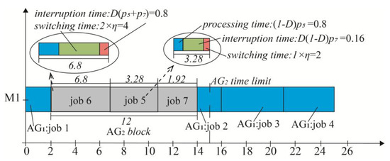
Figure 1. Solution to an illustrative example of Table 1 with parameters $m=1$, $\alpha =1$, $F=15$, $D=0.2$, and $\eta =2$.

3.2. Mathematical Model of the $P_m | (2)mt,C_{max}^{(2)}\le \alpha F |{\displaystyle \sum w_j}{C}_j^{(1)}$ Problem

The problem $P_m | (2)mt,C_{max}^{(2)}\le \alpha F |{\displaystyle \sum w_j}{C}_j^{(1)}$ requires considering the allocation of all jobs on identical parallel machines. Therefore, a mixed-integer programming model (MIP) is provided.

• Variables of MIP along with their brief descriptions

$x_{f,k}^{(2),r}$	Binary variable, if $k\in A{G}_2$ is arranged at $r$ th position of $A{G}_2$ block on machine $f$, $x_{f,k}^{(2),r}=1$; otherwise, $x_{f,k}^{(2),r}=0$.
$x_{f,j}^{(1),r}$	Binary variable, if $j\in A{G}_1$ is arranged at $r$ th position of $A{G}_1$ block on machine $f$, $x_{f,j}^{(1),r}=1$; otherwise, $x_{f,j}^{(1),r}=0$.
$z_f^r$	Binary variable, if the $A{G}_2$ block is inserted after $r$ th position of $A{G}_1$ on machine $f$, $z_f^r=1$; otherwise, $z_f^r=0$.
$t_f^{(2),r}$	Non-negative variable, the duration of $r$ th position of $A{G}_2$ block which is allocated to machine $f$.
$t_f^{(1),r}$	Non-negative variable, the makespan of $r$ th position job from $A{G}_1$ on machine $f$.
$T_f^{(2)}$	Non-negative variable, the duration of the $A{G}_2$ block which is allocated to machine $f$.
$C_j^{(1)}$	Non-negative variable, the makespan of job $j\in A{G}_1$.

Since the position-dependent processing time of jobs from AG₂ is determined by Formula (1), we refer to reference [15] to rewrite the formula by binary variable $x_{f,k}^{(2),r}$ as

$${(1-D)}^{r-1}{\displaystyle \sum _{k\in A{G}_2}{x}_{f,k}^{(2),r}{p}_k}+D{(1-D)}^{r-1}{\displaystyle \sum _{q=r+1}^{n^{(2)}}{\displaystyle \sum _{k\in A{G}_2}{x}_{f,k}^{(2),q}{p}_k}}+\eta {\displaystyle \sum _{q=r+1}^{n^{(2)}}{\displaystyle \sum _{k\in A{G}_2}{x}_{f,k}^{(2),q}}}$$

(6)

where ${(1-D)}^{r-1}{\displaystyle \sum _{k\in A{G}_2}{x}_{f,k}^{(2),r}{p}_k}$ is the actual processing time of job $k\in A{G}_2$; $D{(1-D)}^{r-1}{\displaystyle \sum _{q=r+1}^{n^{(2)}}{\displaystyle \sum _{k\in A{G}_2}{x}_{f,k}^{(2),q}{p}_k}}$ and $\eta {\displaystyle \sum _{q=r+1}^{n^{(2)}}{\displaystyle \sum _{k\in A{G}_2}{x}_{f,k}^{(2),q}}}$ are its interruption time and switching time, respectively. The rewritten expression is adopted to constraint (15).

$$Minimize\hspace{1em}{\displaystyle \sum _{j\in A{G}_1}{w}_j}{C}_j^{(1)}$$

(7)

Subject to

$${\displaystyle \sum _{f=1}^m{\displaystyle \sum _{r=1}^{n^{(2)}}{x}_{f,k}^{(2),r}}}=1 \forall k\in A{G}_2,$$

(8)

$${\displaystyle \sum _{f=1}^m{\displaystyle \sum _{r=1}^{n^{(1)}}{x}_{f,j}^{(1),r}}}=1 \forall j\in A{G}_1,$$

(9)

$${\displaystyle \sum _{k\in A{G}_2}{x}_{f,k}^{(2),r}}\le 1 \forall r=1,\dots ,n^{(2)};f=1,\dots ,m,$$

(10)

$${\displaystyle \sum _{k\in A{G}_1}{x}_{f,j}^{(1),r}}\le 1 \forall r=1,\dots ,n^{(1)};f=1,\dots ,m ,$$

(11)

$${\displaystyle \sum _{k\in A{G}_2}{x}_{f,k}^{(2),r}}\ge {\displaystyle \sum _{k\in A{G}_2}{x}_{f,k}^{(2),r+1}} \forall f=1,\dots ,m;r=1,\dots ,n^{(2)}-1 ,$$

(12)

$${\displaystyle \sum _{j\in A{G}_1}{x}_{f,j}^{(1),r}}\ge {\displaystyle \sum _{j\in A{G}_1}{x}_{f,j}^{(1),r+1}} \forall f=1,\dots ,m;r=1,\dots ,n^{(1)}-1 ,$$

(13)

$${\displaystyle \sum _{r=0}^{n^{(1)}}{z}_f^r}=1 \forall f=1,\dots ,m ,$$

(14)

$$t_f^{(2),r}\ge t_f^{(2),r-1}+{(1-D)}^{r-1}{\displaystyle \sum _{k\in A{G}_2}{x}_{f,k}^{(2),r}}{p}_k+D{(1-D)}^{r-1}{\displaystyle \sum _{q=r+1}^{n^{(2)}}{\displaystyle \sum _{k\in A{G}_2}{x}_{f,k}^{(2),q}}}{p}_k+\eta {\displaystyle \sum _{q=r+1}^{n^{(2)}}{\displaystyle \sum _{k\in A{G}_2}{x}_{f,k}^{(2),q}}} \forall f=1,\dots ,m;r=1,\dots ,n^{(2)} ,$$

(15)

$$t_f^{(1),r}\ge t_f^{(1),r-1}+{\displaystyle \sum _{j\in A{G}_1}{x}_{f,j}^{(1),r}}{p}_j+T_f^{(2)}-(1-z_f^{r-1})M \forall f=1,\dots ,m; r=1,\dots ,n^{(1)} ,$$

(16)

$$t_f^{(1),r}\ge t_f^{(1),r-1}+{\displaystyle \sum _{j\in A{G}_1}{x}_{f,j}^{(1),r}}{p}_j-z_f^{r-1}M \forall f=1,\dots ,m;r=1,\dots ,n^{(1)} ,$$

(17)

$$t_f^{(2),0}=0 \forall f=1,\dots ,m ,$$

(18)

$$t_f^{(1),0}=0 \forall f=1,\dots ,m ,$$

(19)

$$T_f^{(2)}=t_f^{(2),n^{(2)}} \forall f=1,\dots ,m ,$$

(20)

$$t_f^{(1),r}+T_f^{(2)}-(1-z_f^r)M\le \alpha F \forall f=1,\dots ,m;r=0,\dots , n^{(1)} ,$$

(21)

$$C_j^{(1)}\ge t_f^{(1),r}-(1-x_{f,j}^{(1),r})M \forall f=1,\dots ,m;j\in A{G}_1;r=1,\dots ,n^{(1)} ,$$

(22)

The objective function (7) aims to minimize the total weighted completion time of jobs from $A{G}_1$. Constraints (8) and (9) ensure a unique allocation of jobs from $A{G}_1$ and $A{G}_2$. Constraints (10) and (11) guarantee that each position of $A{G}_1$ and $A{G}_2$ can only be occupied by at most one job, thus allowing for some positions to be idle. Constraints (12) and (13) prevent interruptions in the occupation of consecutive positions in $A{G}_1$ and $A{G}_2$. Constraint (14) ensures that each $A{G}_2$ block can only be inserted after one position of $A{G}_1$ on the same machine, with $z_f^r$ representing the insertion position of the $A{G}_2$ block for $A{G}_1$ on machine $f$. Constraint (15) provides the duration of each position associated with multitasking scheduling in the $A{G}_2$ block on each machine. Then the duration of the first position is set to 0 in constraint (18). Constraints (16) and (17) model a lower bound for the job allocated to the $r$th position from $A{G}_1$, using a big-$M$ method to invalidate one of the two constraints. Subsequently, the duration of the first position is set to 0 in constraint (19). Constraint (20) defines the total duration of the $A{G}_2$ block time on machine $f$. Constraint (21) is a hard time limit constraint on each machine. If $z_f^r=1$, the makespan of the $A{G}_2$ block is $t_f^{(1),r}+T_f^{(2)}$, and the makespan must be less than the time limit $\alpha F$. Otherwise, the constraint is invalid. Constraint (22) establishes the relationship between the completion time of a job from $A{G}_1$ and its occupied position. If $x_{f,j}^{(1),r}=0$, constraint (22) is valid; otherwise, $C_j^{(1)}$ corresponds to the position-dependent completion time $t_f^{(1),r}$. For the big-$M$ in constraints (16) and (17) and constraints (21) and (22), it can be set as $M=10\times {\displaystyle {\sum }_{u\in A{G}_2\cup A{G}_2}{p}_u}$. This is because the constraint pairs are mutually exclusive constraints, and big-$M$, as a sufficiently large value, only needs to ensure that when one constraint is active, the other does not affect the solution.

To facilitate better understanding, e.g., the concepts of the “$A{G}_2$ block”, the “duration of $A{G}_2$ block”, and the “inserted position of $A{G}_2$ block”, a simple example is provided in Table 2 and Figure 2.

Table 2. A simple example input data.

Job	1	2	3	4	5	6	7
$p$	2	2	5	4	1	2	3
$w$	6	2	3	2
$A{G}_1$	1	2	3	4
$A{G}_2$	5	6	7

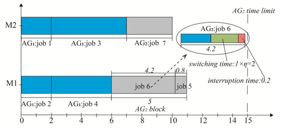
Figure 2. Solution to an illustrative example of Table 2 with parameters $m=2$, $\alpha =1$, $F=15$, $D=0.2$, and $\eta =2$.

The optimal weighted completion time depicted in Figure 2 is $z^{\ast }=2\times 6+2\times 2+7\times 3+6\times 2=49$, with $C_{max}^{(2)}=11<15$. Specifically, Figure 2 shows that jobs $2, 4 \in A{G}_1$ and $6, 5 \in A{G}_2$ are allocated to ${\mathrm{M}}_1$, which demonstrates $x_{1,2}^{(1),1}=1$, $x_{1,4}^{(1),2}=1$ and $x_{1,6}^{(2),1}=1$, $x_{1,5}^{(2),2}=1$. The $A{G}_2$ block consists of jobs $6, 5 \in A{G}_2$, and the insertion position is $z_1^2=1$. In the $A{G}_2$ block, the duration of the first and second positions are

$$\begin{gathered} t_1^{(2),1}\ge t_1^{(2),0}+{(1-D)}^0{x}_{1,6}^{(2),1}{p}_6+D{(1-D)}^0{x}_{1,5}^{(2),2}{p}_5+\eta x_{1,5}^{(2),2}=4.2 \\ {t}_1^{(2),2}\ge t_1^{(2),1}+(1-D)x_{1,5}^{(2),2}{p}_5=4.2+0.8=5. \end{gathered}$$

(23)

Thus, the duration of the $A{G}_2$ block is $T_f^{(2)}=t_1^{(2),2}\ge 5$. Due to the insert position only at $z_1^2=1$, the corresponding position makespan in $A{G}_1$ is

$$\begin{gathered} t_1^{(1),1}\ge t_1^{(1),0}+x_{1,2}^{(1),1}{p}_2=2 , \\ {t}_1^{(1),2}\ge t_1^{(1),1}+x_{1,4}^{(1),2}{p}_4=2+4=6 , \end{gathered}$$

(24)

and the time limit constraint is $t_1^{(1),2}+T_1^{(2)}=6+5\le \alpha F=15$. Therefore, the makespan of jobs 2 and 4 from $A{G}_1$ are

$$C_2^{(1)}\ge t_1^{(1),1}-(1-x_{1,2}^{(1),1})M=2 ,$$

(25)

$$C_4^{(1)}\ge t_1^{(1),2}-(1-x_{1,4}^{(1),2})M =6 .$$

(26)

3.3. Structural Property of the $P_m | (2)mt, C_{\max }^{(2)}\le \alpha F | w_j{C}_j^{(1)}$ Problem

Some similar structure optimal properties are proposed based on the research of Azizoglu and Kirca [44], which is originally mentioned by Elmaghraby and Park [45].

Property 3.

If the last job $j$ belongs to $A{G}_1$, in any optimal schedule the total processing time on any machine is less than

$${\displaystyle \frac{1}{m}}{\displaystyle \sum _{u\in A{G}_1\cup A{G}_2}{p}_u}+{\displaystyle \frac{\eta }{2}}({⌈n^{(2)}/m⌉}^2-⌈n^{(2)}/m⌉)+{\displaystyle \frac{(m-1)p_j}{m}} ,$$

(27)

where $u\in A{G}_1\cup A{G}_2$.

Proof .

Let $j\in A{G}_1$ represent the last job performed on machine $s$ in an optimal schedule, and let $C_s$ denote its makespan. For any other machine $v$, it must satisfy

$$C_s\le C_v+p_j\hspace{1em}\hspace{0.33em}\hspace{0.33em}\hspace{0.33em}1\le v\le m, v\ne s ,$$

(28)

If the inequality did not hold, the total weighted completion time would be decreased by taking $j$ from machine $s$ and putting it last on machine $v$. Thus, by summing the other $(m-1)$ inequalities associated with each $C_v$, it can be concluded that

$$(m-1)C_s\le {\displaystyle \sum _{v=1}^{m-1}{C}_v}+(m-1)p_j ,$$

(29)

$$m{C}_s\le {\displaystyle \sum _{v=1}^{m-1}{C}_v}+C_s+(m-1)p_j.$$

(30)

For each $C_s$ or $C_v$, let $T_s^{(2)}$ and $T_v^{(2)}$ be the total processing time of the $A{G}_2$ block on machines $s$ and $v$. Given the relationship ${\displaystyle \sum _{v=1}^{m-1}{C}_v}+C_s={\displaystyle \sum _{i=1}^{n^{(1)}}{p}_i}+{\displaystyle \sum _{v=1}^{m-1}{T}_v^{(2)}}+T_s^{(2)}$, it can be concluded that $m{C}_s\le {\displaystyle \sum _{i\in A{G}_1}{p}_i}+{\displaystyle \sum _{v=1}^{m-1}{T}_v^{(2)}}+T_s^{(2)}+(m-1)p_j$. Due to the multitasking scheduling formula, ${\displaystyle \sum _{v=1}^{m-1}{T}_v^{(2)}}+T_s^{(2)}$ must satisfy

$${\displaystyle \sum _{k\in A{G}_2}{p}_k}+{\displaystyle \frac{\eta }{2}}[{(n^{(2)})}^2-n^{(2)}]<{\displaystyle \sum _{v=1}^{m-1}{T}_v^{(2)}}+T_s^{(2)}\le {\displaystyle \sum _{k\in A{G}_2}{p}_k}+m\cdot {\displaystyle \frac{\eta }{2}}({⌈n^{(2)}/m⌉}^2-⌈n^{(2)}/m⌉) ,$$

(31)

where ${\displaystyle \sum _{k\in A{G}_2}{p}_k}+{\displaystyle \frac{\eta }{2}}[{(n^{(2)})}^2-n^{(2)}]$ indicates that all jobs from $A{G}_2$ are only allocated to one machine, and ${\displaystyle \sum _{k\in A{G}_2}{p}_k}+m\cdot {\displaystyle \frac{\eta }{2}}({⌈n^{(2)}/m⌉}^2-⌈n^{(2)}/m⌉)$ denotes that $A{G}_2$ jobs are equally allocated to $m$ machines. Utilizing the right side, the upper bound $U_j$ of job $j\in A{G}_1$ is as follows:

$$m{C}_s\le {\displaystyle \sum _{i\in A{G}_1}{p}_i}+{\displaystyle \sum _{k\in A{G}_2}{p}_k}+m\cdot {\displaystyle \frac{\eta }{2}}({⌈n^{(2)}/m⌉}^2-⌈n^{(2)}/m⌉)+(m-1)p_j ,$$

(32)

$$C_s\le U_j={\displaystyle \frac{1}{m}}{\displaystyle \sum _{u\in A{G}_1\cup A{G}_2}{p}_u}+{\displaystyle \frac{\eta }{2}}({⌈n^{(2)}/m⌉}^2-⌈n^{(2)}/m⌉)+{\displaystyle \frac{(m-1)p_j}{m}}$$

(33)

The $U_j$ is the upper bound for a schedule on parallel machines, and the upper bound efficiently cuts useless branches of the two-phase label-setting algorithm. □

4. Branch-and-Price Algorithm

The branch-and-price (B&P) algorithm [46] utilizes the subset-row inequality [47] technique and the label-setting algorithm [48]. This approach is effective for solving routes planning [49] and scheduling problems [50]. This section introduces each part of B&P. Section 4.1 depicts the restricted master problem (RMP). Section 4.2 describes the pricing problem considering the subset-row inequality. A developed label-setting algorithm is introduced in Section 4.3, named the two-phase label-setting algorithm (TP-LS). The rest of the sections detail other procedures of the B&P algorithm.

4.1. Restricted Master Problem

The master problem is to find several partition schedules containing all jobs while minimizing the total weighted completion time of $A{G}_1$. For each partition schedule, the completion time of $A{G}_2$ jobs must satisfy $\alpha F$. Let $\Lambda$ denote the set of all feasible partition schedules and $\lambda \in \Lambda$ be one of partition schedules. Binary decision variable $y_{\lambda }$ indicates whether schedule $\lambda$ is selected or not. $a_{\lambda ,u}$ is a binary indicator indicating whether job $u\in A{G}_1\cup A{G}_2$ is selected or not in schedule $\lambda$. $c_{\lambda }$ is the corresponding weighted completion time. Thus, the formulations of the master problem are shown as follows:

$$\mathrm{Minimize}\hspace{1em}{\displaystyle \sum _{\lambda \in \Lambda }{c}_{\lambda }}{y}_{\lambda } ,$$

(34)

Subject to

$${\displaystyle \sum _{\lambda \in \Lambda }{a}_{\lambda ,u}}{y}_{\lambda }\ge 1\hspace{1em}u\in A{G}_1\cup A{G}_2 ,$$

(35)

$${\displaystyle \sum _{\lambda \in \Lambda }{y}_{\lambda }}\le m ,$$

(36)

$${\displaystyle \sum _{\lambda \in \Lambda }⌊\frac{1}{k}{\displaystyle \sum _{u\in S_r}{a}_{\lambda ,u}}⌋}{y}_{\lambda }\le ⌊{\displaystyle \frac{|S_r|}{k}}⌋\hspace{0.33em}\hspace{0.33em}\hspace{1em}\forall S_r\subset S ,$$

(37)

$$y_{\lambda }\in \{0, 1\}\hspace{0.33em}\hspace{0.33em}\hspace{0.33em}\hspace{1em}\forall \lambda \in \Lambda ,$$

(38)

The objective (34) is to minimize the total cost of selected partition schedules. Constraint (35) guarantees that each job must be selected on parallel machines. Constraint (36) ensures that each machine must select a feasible schedule. Constraint (37) is the subset-row inequality [47]. Usually, $S$ is a job set $A{G}_1\cup A{G}_2$, and $S_r$ is a subset of $S$. It provides a class of cuts to reduce the pricing searches on relaxed solution nodes of the RMP. Constraint (38) is the definition of decision variables.

When the binary variables $y_{\lambda }, \lambda \in \Lambda$ are relaxed as $0\le y_{\lambda }\le 1$, the master problem is relaxed as RMP. In B&P, a series of dual variables and relaxed linear solutions are obtained from the RMP. Let $C(c_{\lambda }\in C)$ be a vector associated with the objective coefficients and let $A(a_{\lambda ,u}\in A)$ be a binary indicator matrix according to constraint (35). Vector $C$ and matrix $A$ will be mentioned frequently in Section 4.

4.2. Pricing Problem

The basic idea of B&P is to start with a small subset of high-quality feasible solutions to form up the RMP. The RMP is solved to obtain its dual solution. The pricing problem then aims to find columns with negative reduced costs, which are subsequently added to the RMP. Let ${\pi }_u$ be the dual variables corresponding to constraint (35) and let $\sigma$ be related to constraint (36). Consequently, ${\gamma }_{S_r}$ is the dual variable of constraint (37). The reduced cost $r_{\lambda }$ of schedule $\lambda$ is defined by

$$r_{\lambda }=c_{\lambda }-\sigma -{\displaystyle \sum _{u\in Z_{\lambda }^{(1)}\cup Z_{\lambda }^{(2)}}{\pi }_u}-{\displaystyle \sum _{S_r\subset S}{\chi }_{\lambda ,S_r}}\cdot {\gamma }_{S_r} ,$$

(39)

where $c_{\lambda }$ is the total weighted completion time of jobs belonging to $A{G}_1$. $Z_{\lambda }^{(1)}$ and $Z_{\lambda }^{(2)}$ are sequences indicating job processing orders for $A{G}_1$ and $A{G}_2$, respectively. ${\chi }_{\lambda ,S_r}$ is a binary variable. If at least two jobs of $S_r$ are in $Z_{\lambda }^{(1)}\cup Z_{\lambda }^{(2)}$, then ${\chi }_{\lambda ,S_r}=1$; if at most one job of $S_r$ is in $Z_{\lambda }^{(1)}\cup Z_{\lambda }^{(2)}$, then ${\chi }_{\lambda ,S_r}=0$. Because $\sigma$ is a constant, the objective function (39) of the pricing problem becomes $c_{\lambda }-{\displaystyle \sum _{u\in Z_{\lambda }^{(1)}\cup Z_{\lambda }^{(2)}}{\pi }_u}-{\displaystyle \sum _{S_r\subset S}{\chi }_{\lambda ,S_r}}\cdot {\gamma }_{S_r}$.

4.3. Two-Phase Label-Setting Algorithm

The two-phase label-setting (TP-LS) algorithm is proposed in this section. The first phase only involves the $A{G}_1$ jobs, and the labels can be treated as root nodes. The second phase only associates with $A{G}_2$ jobs, and the labels are regarded as leaf nodes. The second phase starts with a transferred label $l_i^{(1)}$ of the first phase, performs a search, and outputs the best-found result. In short, during the searching process of every root node, all leaf nodes must be considered.

• Symbols of the first phase label-setting algorithm

$l_i^{(1)}$	The label associates with node $i$, and it ends with job, where $i\in A{G}_1$.
$Z_i^{(1)}$	The partitioning schedule of label $l_i^{(1)}$, which only includes the set of jobs belonging to $A{G}_1$ and ends with job $i$.
$R_i^{(1)}$	The set of jobs that are available and can be extended at $A{G}_1$ job $i$.
$r_i^{(1)}$	The reduced cost of label $l_i^{(1)}$.
$FPLS$	The recursive algorithm of the first phase label-setting algorithm, where the inputs are $Z_i^{(1)},R_i^{(1)},r_i^{(1)}$.

• Symbols of the second phase label-setting algorithm

$l_k^{(2)}$	The label associates with node $k$, and ends with job $k$, where $k\in A{G}_2$.
$Z_k^{(2)}$	The partitioning schedule of label $l_k^{(2)}$, which only includes the set of jobs belonging to $A{G}_2$ and ends with job $k$.
$R_k^{(2)}$	The set of jobs that are available and can be extended at $A{G}_2$ job $k$.
$r_k^{(2)}$	The reduced cost of label $l_k^{(2)}$.
$Z_k$	The overall schedule includes the transferred $Z_k^{(1)}$ and $Z_k^{(2)}$, and it is obtained by PolALG.
$T_k^{(2)}$	The duration of the $A{G}_2$ block.
$t_k^{(2)}$	The completion time of the $A{G}_2$ job $k$, where $k\in A{G}_2$.
$c_k^{(2)}$	The total weighted completion time of $A{G}_1$ jobs at $SPLS$ label $l_k^{(2)}$.
$SPLS$	The recursive algorithm of the second phase of the label-setting algorithm, where the inputs are $Z_j^{(1)},r_{\min }^{(2)},Z_k^{(2)},R_k^{(2)},T_k^{(2)},t_k^{(2)}$, and $r_{\min }^{(2)}$ is set to $r_{\min }^{(2)}=+\propto$ before $SPLS$ starts.

4.3.1. First Phase Label-Setting Algorithm

In the first phase label-setting (FPLS) algorithm, a label represents a feasible partition schedule of $A{G}_1$ jobs. Suppose that the set ${\mathcal{L}}^{(1)}$ contains all labels associated with $A{G}_1$. Let job $i\in A{G}_1$ be a node indicating a path ended at job $i$, and $l_i^{(1)}=(Z_i^{(1)},R_i^{(1)},r_i^{(1)})$ be a label associated with node $i$. Let $l_j^{(1)}=(Z_j^{(1)},R_j^{(1)},r_j^{(1)})$ be a consecutive successor label of $l_i^{(1)}$. From $l_i^{(1)}$ to $l_j^{(1)}$, the extension equations are formulated as follows:

$$Z_j^{(1)}=Z_i^{(1)}\cup \left\{j\right\} ,$$

(40)

$$R_j^{(1)}=R_i^{(1)}\backslash \left\{j\right\} ,$$

(41)

$$r_j^{(1)}=r_{\min }^{(2)}\leftarrow SPLS(Z_j^{(1)},r_{\min }^{(2)},Z_0^{(2)},R_0^{(2)},T_0^{(2)},t_0^{(2)}) ,$$

(42)

where $Z_i^{(1)}\cup \left\{j\right\}$ denotes that $j$ is inserted at the end of sequence $Z_i^{(1)}$, and $R_i^{(1)}\backslash \left\{j\right\}$ represents that $j$ is removed from the sequence $R_i^{(1)}$. Moreover, $r_j^{(1)}=r_{\min }^{(2)}\leftarrow SPLS(Z_j^{(1)},r_{\min }^{(2)},Z_0^{(2)},R_0^{(2)},T_0^{(2)},t_0^{(2)})$ indicates that $r_j^{(1)}$ is obtained by the second phase label-setting algorithm. $r_{\min }^{(2)}$ is the minimum reduced cost, obtained by exploring all leaf nodes of SPLS. In Equation (42), the inputs of SPLS, such as $r_{\min }^{(2)},Z_0^{(2)},R_0^{(2)},T_0^{(2)},t_0^{(2)}$, are of dummy label $l_0^{(2)}$, which will be detailed in Algorithm 2.

Lemma 1.

 The label $l_i^{(1)}$ dominates $l_j^{(1)}$ if $r_i^{(1)}\le r_j^{(1)}$ , where $i,j\in A{G}_1$.

Proof .

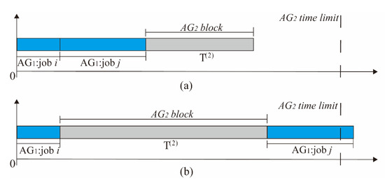
Suppose that the starting time of the last job in $Z_j^{(1)}\in l_j^{(1)}$ is $e_j$. If $r_i^{(1)}<r_j^{(1)}$, we need to discuss two cases of the labels. ① In case 1, $T^{(2)}$ of the $A{G}_2$ block from SPLS is not a long duration so that the time limit $\alpha F$ is sufficient for allocating $A{G}_2$ block after job $j$. We have $r_j^{(1)}-r_i^{(1)}=w_j(e_j+p_j)-{\pi }_j=\Delta r_j>0$ (as shown in Figure 3a). ② In case 2, $T^{(2)}$ of the $A{G}_2$ block from SPLS is a long duration, and the time limit $\alpha F$ is tight. In this scenario, the block of $A{G}_2$ is scheduled between jobs $i$ and $j$, and we have $r_j^{(1)}-r_i^{(1)}=w_j(e_j+T^{(2)}+p_j)-{\pi }_j>{\Delta }^{\prime }{r}_j>\Delta r_j>0$ (as shown in Figure 3b). For both ${\Delta }^{\prime }{r}_j>0$ and $\Delta r_j>0$, it indicates that the reduced cost increment (${\Delta }^{\prime }{r}_j$ or $\Delta r_j$) of job $j\in A{G}_1$ =has a negative impact on searching for minimum reduced cost. As a result, it is evident that label $l_i^{(1)}$ dominates $l_j^{(1)}$. □

Figure 3. Typical examples of a successor label $l_q^{(1)}$ for Lemma 1: (a) an illustrative Gannt chart of case 1; (b) an illustrative Gannt chart of case 2.

Algorithm 2 First phase label-setting algorithm FPLS

Input $Z_i^{(1)},R_i^{(1)},r_i^{(1)}$

Output $r_{\min },Z_{\min },c_{\min }$

1: while $|R_i^{(1)}|>0$ do

2:   $j=R_i^{(1)}[1]$, $R_i^{(1)}\backslash \left\{j\right\}$

3:   Initialize consecutive label $l_j^{(1)}:Z_j^{(1)}=Z_i^{(1)}\cup \left\{j\right\},R_j^{(1)}=R_i^{(1)},r_j^{(1)}=0$

4:   Initialize dummy label $l_0^{(2)}:Z_0^{(2)}=(),R_0^{(2)}=A{G}_2,T_0^{(2)}=0,t_0^{(2)}={\displaystyle {\sum }_{q\in Z_j^{(1)}}{p}_q}$

5:   $r_{\min }^{(2)}=+\propto ,Z_{\min }^{(2)}=(),c_{\min }^{(2)}=()$/* Initialize data structure of SPLS */

6:   $r_j^{(1)}=r_{\min }^{(2)},Z_{\min }^{(2)},c_{\min }^{(2)}\leftarrow SPLS(Z_j^{(1)},r_{\min }^{(2)},Z_0^{(2)},R_0^{(2)},T_0^{(2)},t_0^{(2)})$

7:   if $r_{\min }>r_i^{(1)}$ then

8:     $r_{\min }=r_i^{(1)},Z_{\min }=Z_{\min }^{(2)},c_{\min }=c_{\min }^{(2)}$

9:   end if

10:    if $r_j^{(1)}\le r_i^{(1)}$ then / *Lemma 1 */

11:      $FPLS(Z_j^{(1)},R_j^{(1)},r_j^{(1)})\hspace{0.33em}\hspace{0.33em}\hspace{0.33em}$/ * Start next recursion */

12:    end if

13: end while

Algorithm 2 FPLS is the primary algorithm of TP-LS. The FPLS starts from a dummy label $l_0^{(1)}$, where $Z_0^{(1)}=(),r_0^{(1)}=0$, and $R_0^{(1)}$ contains $A{G}_1$ jobs according to the SWPT order. FPLS is a recursive function that calls itself repeatedly. The data structures $r_{\min },Z_{\min },c_{\min }$ for storing the best-found solutions need to be initialized before FPLS starts; that is,$r_{\min }=+\propto ,Z_{\min }=(),c_{\min }=()$. Similarly, lines 4–5 in FPLS initialize the dummy label and the data structure of SPLS. The best-found solutions from FPLS are obtained in line 6, and lines 7–9 are used to store them.

4.3.2. Second Phase Label-Setting Algorithm

In the second phase label-setting (SPLS) algorithm (Algorithm 3), let ${\mathcal{L}}^{(2)}$ be the set of $A{G}_2$ labels based on a transferred label $l_j^{(1)}$ of $A{G}_1$, which contains all labels associated with $A{G}_2$. Let $k$ be a node indicating a path ended at job $k\in A{G}_2$, and $l_k^{(2)}=(Z_k^{(2)},R_k^{(2)},Z_k,T_k^{(2)},t_k^{(2)},c_k^{(2)},r_k^{(2)})$ be a label associated with node $k$. Let $l_h^{(2)}$ be a consecutive successor label of $l_k^{(2)}$. From $l_k^{(2)}$ to $l_h^{(2)}$, the extension equations are formulated as follows:

$$Z_h^{(2)}=Z_k^{(2)}\cup \left\{h\right\} ,$$

(43)

$$R_h^{(2)}=R_k^{(2)}\backslash \left\{h\right\} ,$$

(44)

$$Z_h,T_h^{(2)},t_h^{(2)},c_h^{(2)}\leftarrow PolALG(Z_j^{(1)},Z_h^{(2)}) ,$$

(45)

$$r_h^{(2)}=c_h^{(2)}-{\displaystyle \sum _{u\in Z_j^{(1)}\cup Z_h^{(2)}}{\pi }_u}-{\displaystyle \sum _{S_r\subset S}{\chi }_{h,S_r}}\cdot {\gamma }_{S_r} ,$$

(46)

where Formula (45) indicates that Algorithm 1 is adopted to obtain the schedule associated with $Z_j^{(1)}$ and $Z_h^{(2)}$, the duration of $Z_h^{(2)}$, the makespan, and the total weighted completion time. In short, each available leaf node of SPLS needs to adopt PolALG to quickly obtain the corresponding results. ${\chi }_{h,S_r}$ of Equation (46) is a binary indicator indicating whether there are at least two jobs of $S_r$ in $Z_h$. After generating the overall schedule $Z_h$, we provide a binary vector ${\chi }_h$ by inspecting both $S_r$ and $Z_h$. Therefore, the length of the vector ${\chi }_h$ is the same as that of $S$, and every ${\chi }_{h,S_r}$ comes from ${\chi }_h$.

Lemma 2.

If the last job of the overall schedule $Z_h\in l_h^{(2)}$ belongs to $A{G}_1$, $l_h^{(2)}$ is dominated if $t_h^{(2)}$ is more than

$${\displaystyle \frac{1}{m}}{\displaystyle \sum _{u\in A{G}_1\cup A{G}_2}{p}_u}+{\displaystyle \frac{\eta }{2}}({⌈n^{(2)}/m⌉}^2-⌈n^{(2)}/m⌉)+{\displaystyle \frac{(m-1)p_j}{m}},$$

(47)

where $j\in A{G}_1$ is the last job of $Z_h$ , and $u\in A{G}_1\cup A{G}_2$ is the job belonging to $A{G}_1$ or $A{G}_2$.

Lemma 2 is the dominance rule corresponding to structural Property 3 (see Section 3.3).

Lemma 3.

The label $l_k^{(2)}$ dominates $l_h^{(2)}$ if $T_k^{(2)}\le \alpha F$ and $T_h^{(2)}>\alpha F$, where $k,h\in A{G}_2$.

Because of the strict due-date constraint $C_{max}^{(2)}\le \alpha F$, it implies that the duration of any search label cannot exceed $\alpha F$. It is obvious that any duration ($T_h^{(2)}$) of $A{G}_2$ cannot be larger than the due date $\alpha F$, which leads to Lemma 3. In addition, Lemma 4 is provided to omit useless leaf nodes for the searching of SPLS.

Lemma 4.

The label $l_k^{(2)}$ dominates $l_h^{(2)}$ if $r_k^{(2)}\le r_h^{(2)}$, where $k,h\in A{G}_2$.

Proof .

If $\Delta r_h>0$, the allocation of job $h\in A{G}_2$ cannot decrease the reduced cost, and $l_k^{(2)}$ dominates $l_h^{(2)}$. Here, two cases of SPLS need to be discussed. ➀ In case 1, $T^{(2)}$ of the $A{G}_2$ block at label $l_k^{(2)}$ is not a long duration, so the time limit $\alpha F$ is sufficient (see Figure 4a). However, after allocating job $h$ to the $A{G}_2$ block, we have $\Delta r_h=w_j(T^{(2)}+p_h)-{\pi }_h\ge 0$. ➁ In case 2, $T^{(2)}$ is a long duration, so the time limit $\alpha F$ is tight (see Figure 4b). After allocating job $h$ to the $A{G}_2$ block, we have $\Delta r_h=w_j{p}_h-{\pi }_h\ge 0$. In both cases, it satisfies $\Delta r_h=r_h^{(2)}-r_k^{(2)}>0$. □

Figure 4. Typical examples of a successor label $l_h^{(2)}$ for Lemma 4: (a) an illustrative Gannt chart of case 1; (b) an illustrative Gannt chart of case 2.

Algorithm 3 Second phase label-setting algorithm SPLS

Input:  $Z_j^{\left(1\right)}, r_{\min }^{\left(2\right)}, Z_k^{\left(2\right)},{ R}_k^{\left(2\right)},{ T}_k^{\left(2\right)},{ t}_k^{\left(2\right)}$

Output:  $r_{\min }^{\left(2\right)}, { Z}_{\min }^{\left(2\right)},{ c}_{\min }^{\left(2\right)}$

1: while $|R_k^{(2)}|>0$ do

2:     $h=R_k^{(2)}[1]$, $R_k^{(2)}\backslash \left\{h\right\}$

3:     Initialize consecutive label $l_h^{(2)}:Z_h^{(2)}=Z_k^{(2)}\cup \left\{h\right\},R_h^{(2)}=R_k^{(2)}$

4:     $T_h^{(2)},c_h^{(2)},t_h^{(2)},Z_h\leftarrow PolALG(Z_j^{(1)},Z_h^{(2)})$

5:     Obtain reduced cost: $r_h^{(2)}=c_h^{(2)}-{\displaystyle \sum _{u\in Z_j^{(1)}\cup Z_h^{(2)}}{\pi }_u}-{\displaystyle \sum _{S_r\subset S}{\chi }_{h,S_r}}\cdot {\gamma }_{S_r}$

6:     if $|c_{\min }^{(2)}|\ge Q$ then

7:        $Z_{\min }^{(2)}.pop\_back{()}^a$,$c_{\min }^{(2)}.pop\_back{()}^a$

8:     end if

9:     if $r_{\min }^{(2)}>r_h^{(2)}$ then

10:       $r_{\min }^{(2)}=r_h^{(2)},c_{\min }^{(2)}=\left\{c_h^{(2)}\right\}\cup c_{\min }^{(2)b}$,$Z_{\min }^{(2)}=Z_h\cup Z_{\min }^{(2)b}$

11:     end if

12:     if $T_h^{(2)}<\alpha F$ then / *Lemma 3 */

13:         if $r_h^{(2)}\le r_k^{(2)}$ then / *Lemma 4 */

14:          $q=Z_h.back{()}^c$

15:          if $q$ is in $A{G}_1$ and $t_h^{(2)}<U_q$ then / *Lemma 2 */

16:           $SPLS(Z_j^{(1)},r_{\min }^{(2)},Z_h^{(2)},R_h^{(2)},T_h^{(2)},t_h^{(2)})$ / * Start next recursion */

17:          end if

18:        end if

19:      end if

20: end while

a Remove the last item from the sequence. b Insert $c_h^{(2)}$ at the head of $c_{\min }^{(2)}$. c Obtain the last item from the sequence.

In Algorithm 2, SPLS starts at dummy label $l_0^{(2)}$ and transferred label $l_j^{(1)}$ of FPLS and supplies the minimum reduced cost for FPLS after searching all leaf nodes. Line 4 in SPLS obtains the optimal overall schedule by Algorithm 1. Lines 12–19 apply the proposed Lemmas 2–4 to prune useless leaf nodes, thereby speeding up the algorithm.

In general, the pricing problem may have multiple optimal solutions. Adding multiple columns to the RMP at each iteration can improve performance by reducing computational time [51]. Here, let $r_{\min }$ be the best-found reduced cost of TP-LS, then $S_{\min }$ and $c_{\min }$ are queues containing a series of high-quality solutions for the pricing problem. $Q$ is the queue size, and it is set to 10. For a better understanding, Table 3 and Table 4 provide a simple example to illustrate the procedure of the TP-LS algorithm.

Table 3. A simple example of the pricing problem corresponds to the input data of Table 2.

Job	1	2	3	4	5	6	7
$\pi$	18.0	10.0	21.0	14.0	0.0	0.0	2.0
$\sigma$	−6.0
$S_r$	{1,2,7}	{2,4,7}
${\gamma }_r$	−2.0	−2.0
$U_j$	12.5	12.5	14.0	12.0

Table 4. The detailed results of the pricing problem of Table 2.

${\mathit{Z}}_{\mathit{k}}^{\left(2\right)}$	${\mathit{r}}_{\mathit{k}}^{\left(2\right)}$	${\mathit{c}}_{\mathit{k}}^{\left(2\right)}$	${\mathit{C}}_{\mathbf{max}}$	${\mathit{C}}_{\mathbf{max}}^{\left(2\right)}$	${\mathit{T}}^{\left(2\right)}$
$\varnothing$	−6.0	15.0	5.0	5.0	0.0
(5)	−6.0	15.0	6.0	6.0	1.0
(5,6)	−6.0	15.0	10.0	10.0	5.0
(5,6,7)	28.0	51.0	17.0	12.0	12.0
(5,7)	−8.0	15.0	11.0	11.0	6.0
(6)	−6.0	15.0	7.0	7.0	2.0
(6,7)	−8.0	15.0	12.0	12.0	7.0
(7)	−8.0	15.0	8.0	8.0	3.0

Table 3 shows the dual variable values from one iteration of the B&P algorithm. In Table 3, $U_j$ is the time upper bound of job $j\in A{G}_1$ according to Lemma 2. For example, the time upper bound of job $3\in A{G}_1$ in Figure 5c can be obtained by

$$U_3={\displaystyle \frac{1}{2}}\times (p_1+\dots +p_7)+{\displaystyle \frac{2}{2}}({⌈3/2⌉}^2-⌈3/2⌉)+{\displaystyle \frac{(2-1)\times 5}{2}}=9.5+2+2.5=14.$$

(48)

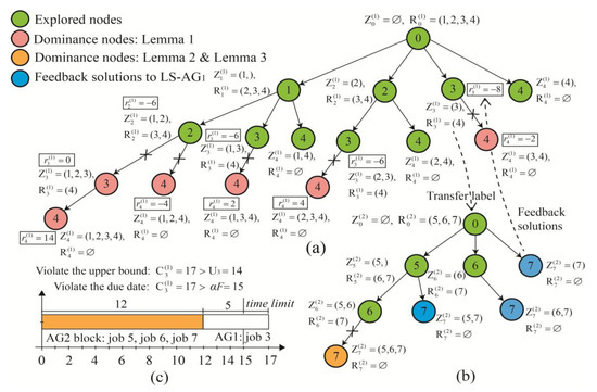
Figure 5. The recursive paths of the pricing problem in Table 2: (a) the recursive paths of FPLS; (b) the recursive paths of SPLS; (c) the violation node of Lemma 2 in SPLS recursive paths.

Indeed, before starting a round of iteration, the time upper bounds of $A{G}_1$ jobs are obtained by Lemma 2. In Figure 5, both FPLS and SPLS are based on depth first search order. On the left-most branch in Figure 5a, both $r_4^{(1)}=14$ and $r_3^{(1)}=0$ are larger than $r_2^{(1)}=-6$; this implies that label $l_2$ dominates $l_3$ and $l_4$, which demonstrates the effectiveness of Lemma 1. Figure 5b depicts the recursive paths when the transferred $A{G}_1$ label is $Z_3^{(1)}=(3)$, and Table 4 lists results of all nodes in Figure 5b. $C_{\max }$, $C_{\max }^{(2)}$, and $T^{(2)}$ represent the makespan, the completion time of $A{G}_2$, and the duration of $A{G}_2$. The schedules with the same minimum reduced cost can be found in Table 4, such as $(5,7)$, $(6,7)$, and $(7)$. For explaining Lemma 2 and Lemma 3, Figure 5c depicts the violation of node 7 in Figure 5b. The $A{G}_2$ jobs are 5, 6, and 7, and the $A{G}_2$ block time is $T^{(2)}=12$. Thus, the completion time of job 3 is $C_3^{(1)}=17$, which violates the upper bound $U_3=14$ of Lemma 2 and the due date $\alpha F=15$ of Lemma 3. As mentioned in Section 4.2, $\sigma$ is a constant and is not considered during the searching process. Finally, the final results of the pricing problem are $r_{\min }=-8-\sigma =-2$ and $c_{\min }=(15.0,15.0,15.0,24.0,24.0,24.0,24.0,33.0,33.0,33.0)$.

4.4. Primary Heuristic

Because the common time limit ($\alpha F$) in this paper is regarded as a hard constraint, obtaining a series of initial solutions without violating deadlines is a laborious work. By utilizing Algorithm 1, this procedure aims to obtain a series of feasible solutions with good qualities. Let $S^{(1)}=A{G}_1$ and $S^{(2)}=A{G}_2$. Then, $S^{(1)}$ and $S^{(2)}$ are randomly shuffled. For the first $m-1$ machines, extract $⌊{\displaystyle \frac{|S^{(1)}|}{m}}⌋$ and $⌊{\displaystyle \frac{|S^{(2)}|}{m}}⌋$ jobs from $S^{(1)}$ and $S^{(2)}$, respectively. For the $m$ th machine, extract all remaining jobs from $S^{(1)}$ and $S^{(2)}$, respectively. Note that the extracted job sequences for each machine are $Z_k^{(1)}, Z_k^{(2)}, k=1,\dots ,m$. Call Algorithm 1 $PolALG(Z_k^{(1)}, Z_k^{(2)})$ to obtain the schedule $S_k^{\ast }$ and the weighted completion time $c_k^{\ast }$. If the result violates the time limit ($\alpha F$), reshuffle $S^{(1)}$ and $S^{(2)}$ and perform the above procedures again; otherwise, transform $S_k^{\ast }$ to a binary vector and add it to the coefficient matrix $A$.

4.5. Branching Rule

To guarantee integrality of solutions, we execute branching on the relaxed variables ${\overline{y}}_{\lambda }(0<{\overline{y}}_{\lambda }<1)$. The branching rule does not change the structure of the pricing problem. Given a series of RMP solutions (${\overline{y}}_{\lambda }, 0<{\overline{y}}_{\lambda }<1, \lambda \in \Lambda$), the solution set may have fractional values. Let $\theta (\theta \in \mathrm{\Theta })$ be the index $\lambda$ of fractional values of ${\overline{y}}_{\lambda }\in (0,1)$ and $\kappa (\kappa \in K)$ be the index $\lambda$ of integer values of ${\overline{y}}_{\lambda }\in \{0,1\}$, $\mathrm{\Theta }\cup K=\Lambda$. Hence, two branching rules are adopted in hierarchy.

Branching on jobs. We branch on the value of ${\overline{y}}_{\theta }$ close to 0.5. Two child nodes of ${\overline{y}}_{\theta }$, which are set to 0 and 1 (the integer child node of ${\overline{y}}_{\theta }$ is denoted as ${\overline{y}}_{\theta }^{+}$), are generated by forbidding or selecting the partitioning schedule $\lambda$ separately. By forcing all ${\overline{y}}_{\theta }^{+}$ to satisfy that ${\displaystyle \sum _{\theta \in \mathrm{\Theta }}{a}_{u,\theta }}{\overline{y}}_{\theta }^{+}=1$, a series of integer ${\overline{y}}_{\theta }^{+}$ is obtained.

Branching on the number of machines. The obtained ${\overline{y}}_{\theta }^{+}$ must obey that ${\displaystyle \sum _{\theta \in \mathrm{\Theta }}{\overline{y}}_{\theta }^{+}}+{\displaystyle \sum _{\kappa \in K}{\overline{y}}_{\kappa }}=m$. Otherwise, the branching on jobs is repeated to guarantee that ${\overline{y}}_{\theta }^{+}$ must satisfy ${\displaystyle \sum _{\theta \in \mathrm{\Theta }}{\overline{y}}_{\theta }^{+}}+{\displaystyle \sum _{\kappa \in K}{\overline{y}}_{\kappa }}=m$.

The two branching rules are adopted in hierarchy until a ground of ${\overline{y}}_{\theta }^{+}$ do not violate the constraints. Specifically, the branching on jobs guarantees its integer child nodes to satisfy constraint (35) of the RMP, and branching on the number of machines pledges the integer child nodes to satisfy constraint (36). The integer solutions (the selections: ${\overline{y}}_{\theta }^{+}(\theta \in \mathrm{\Theta })$, the cost: ${\displaystyle \sum _{\theta \in \mathrm{\Theta }}{\overline{y}}_{\theta }^{+}}{c}_{\theta }+{\displaystyle \sum _{\kappa \in K}{\overline{y}}_{\kappa }}{c}_{\kappa }$) are stored.

4.6. The Structure of the Branch-and-Price Algorithm

The basic idea of B&P is to start with a subset of high-quality feasible solutions to form the RMP. van den Akker et al. [52] emphasized that running the primary heuristic between 2000 and 5000 times and storing the 10 best-found solutions achieves better efficiency. The B&P algorithm can be summarized as follows: the pricing problem aims to find a new set of columns with the minimum negative reduced cost, which is then added in the RMP.

Step 1	Perform the primary heuristic (see Section 4.4) 5000 times, then store the 10 best solutions found. Initial coefficient matrix $\mathrm{C}$, $\mathrm{A}$ and $S$ of the RMP; go to Step 2.
Step 2	Solve the RMP and obtain the dual values ($\pi$,$\gamma$ and $\sigma$). Initialize the dummy label $l_0^{(1)}=(Z_0^{(1)},R_0^{(1)},r_0^{(1)})$ of Algorithm 2, where $Z_0^{(1)}=\varnothing$, $R_0^{(1)}=A{G}_1$, and $r_0^{(1)}=0$, and perform Algorithm 2. Simultaneously, input $Z_j^{(1)},r_{\min }^{(2)},Z_k^{(2)},R_k^{(2)},T_k^{(2)},t_k^{(2)}$ from Algorithm 1 to Algorithm 2, then perform Algorithm 2 (see Section 4.3). Obtain a set of pricing solutions $r_{\min }$,$c_{\min }$, and $Z_{\min }$; go to Step 3.
Step 3	If the reduced cost $r_{\min }-\sigma <\epsilon$, transform $Z_{\min }$ as a set of binary vectors, then add $c_{\min }$ and the binary vectors into the coefficient matrix ($C$ and $A$) of the RMP and go to Step 2; otherwise, terminate B&P iteration. Go to Step 4.
Step 4	If ${\overline{y}}_{\lambda },\lambda \in \Lambda$ has fractional values, perform the branching rule (see Section 4.5), which obtains a series of integer solutions of ${\overline{y}}_{\lambda },\lambda \in \Lambda$ and the corresponding objective value; otherwise, record solutions of ${\overline{y}}_{\lambda },\lambda \in \Lambda$ and the corresponding objective value. Output all solutions.

Figure 6 provides a comprehensive depiction of the operational workflow of the B&P approach, while explicitly elucidating the intricate relationships among its constituent steps. For the reduced cost, B&P can suffer from poor convergence due to the so-called tailing off phenomenon, where the objective values tend to be very close (but not equal) to the final LP value for numerous iterations [53]. Here, we do not compare the reduced cost against zero but check whether it is greater than a small number $\epsilon$ (e.g., $\epsilon =-0.5$).

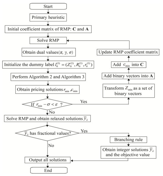
Figure 6. Flowchart of the branch-and-price approach structure.

5. Computational Experiments

The B&P algorithm was coded by C++ and compiled with MinGW. The MIP and the proposed original RMP were solved by IBM ILOG CPLEX 12.9 solver. All computational experiments were solved by a PC with a 2.80 GHz Intel Pentium Core (TM) i7-7700HQ CPU and 8 GB of RAM. In order to explore the performance of B&P, the large-sized instance problems were solved under a time limit of 7200 s (2.0 h).

5.1. Description of Datasets

To evaluate the effectiveness and optimality of B&P, two sets of instance problems were adopted. The first dataset was generated from the literature [13]. The proposed MIP (see Section 3.2) is able to solve $P_m | (2)mt, C_{\max }^{(2)}\le \alpha F | w_j{C}_j^{(1)}$ and utilizes one of the state-of-the-art solvers (CPLEX 12.9) as the standard comparison. In dataset 1, each group of jobs has $\alpha \in \{1.0, 1.5, 2.0\}$ and $q\in \{0.25, 0.50, 0.75\}$, where $q$ represents the percentage of $A{G}_1$ job out of the total number of jobs. $D$ and $\eta$ are set to 0.1 and 0.5, respectively.

The second dataset consists of large-sized instance problems related to multitasking. The processing time $p_j$, weight $w_j$, and $A{G}_2$ time limit $F$ were randomly generated as follows:$p_j~U[1,100]$, $w_j~U[1,100]$, and $F~U(⌈{\displaystyle \sum _{j=1}^n{p}_j}/m⌉,{\displaystyle \sum _{j=1}^n{p}_j})$, respectively. To simulate the short-term and urgent online tasks, each group of jobs is assigned parameters for $\alpha \in \{0.8,1.0\}$ and $q\in \{0.50,0.75\}$, where $q$ represents the percentage of $A{G}_1$ jobs out of total jobs. The interruption factor $D$ is set to 0.2 and $\eta$ is set to 2. To our best knowledge, there is no exact approach to completely solve these problems associated with multitasking scheduling, even for the MIP model.

5.2. Comparison Results of $P_m | (2)mt, C_{\max }^{(2)}\le \alpha F |{\displaystyle \sum w_j}{C}_j^{(1)}$ Problems

Table 5 and Table 6 report the results of instance problems with jobs 10 and 11, respectively. The tables include information about optimality and CPU time for each combination $(n, m, \alpha , q)$ of instances. $ub$ displays the objective values obtained by MIP and B&P using binary variables. $lb$ represents the objective values obtained by B&P using relaxed binary variables in the RMP. $gap$ is calculated by $(ub-lb)/lb$, reflecting the tightness of B&P’s optimality. The objective values are obtained by B&P using relaxed binary variables in the RMP. $t(s)$ shows the running CPU time.

Table 5. B&P compared to MIP with $n=10$, $D=0.10$, and $\eta =0.50$.

Parameters				MIP		B&P
n	m	α	q	ub	t(s)	lb	ub	gap	t(s)
10	2	1.0	0.25	685.00	0.19	685.00	685.00	0.00	4.51
			0.50	425.00	1.17	425.00	425.00	0.00	4.02
			0.75	586.00	18.03	586.00	586.00	0.00	3.83
		1.5	0.25	160.00	0.98	160.00	160.00	0.00	2.51
			0.50	335.00	1.49	335.00	335.00	0.00	3.12
			0.75	586.00	41.20	586.00	586.00	0.00	3.56
		2.0	0.25	160.00	0.75	160.00	160.00	0.00	2.73
			0.50	335.00	0.62	335.00	335.00	0.00	3.00
			0.75	586.00	27.72	586.00	586.00	0.00	4.33
	3	1.0	0.25	480.00	3.07	472.50	480.00	0.02	2.93
			0.50	345.00	5.61	345.00	345.00	0.00	3.10
			0.75	466.00	63.84	466.00	466.00	0.00	3.68
		1.5	0.25	140.00	0.61	140.00	140.00	0.00	3.00
			0.50	280.00	4.18	280.00	280.00	0.00	2.93
			0.75	463.00	46.97	463.00	463.00	0.00	3.43
		2.0	0.25	140.00	0.19	140.00	140.00	0.00	2.89
			0.50	280.00	4.91	280.00	280.00	0.00	3.27
			0.75	463.00	80.62	463.00	463.00	0.00	3.53
	4	1.0	0.25	287.50	2.66	287.50	287.50	0.00	2.61
			0.50	300.00	3.35	300.00	300.00	0.00	2.90
			0.75	411.00	302.89	411.00	411.00	0.00	3.72
		1.5	0.25	140.00	0.47	140.00	140.00	0.00	2.73
			0.50	250.00	11.17	250.00	250.00	0.00	3.29
			0.75	410.00	600.85	410.00	410.00	0.00	3.77
		2.0	0.25	140.00	1.43	140.00	140.00	0.00	2.90
			0.50	250.00	5.93	250.00	250.00	0.00	3.51
			0.75	410.00	366.35	410.00	410.00	0.00	3.75
Avg.				352.35	59.16	352.07	352.35	0.00	3.32

Table 6. B&P compared to MIP with $n=11$, $D=0.10$, and $\eta =0.50$.

Parameters				MIP		B&P
n	m	α	q	ub	t(s)	lb	ub	gap	t(s)
11	3	1.0	0.25	560.00	13.18	552.50	560.00	0.01	2.86
			0.50	467.50	8.58	459.17	467.50	0.02	3.84
			0.75	510.00	393.00	510.00	510.00	0.00	4.73
		1.5	0.25	140.00	0.74	140.00	140.00	0.00	2.65
			0.50	425.00	16.25	425.00	425.00	0.00	3.25
			0.75	502.00	235.24	502.00	502.00	0.00	3.59
		2.0	0.25	140.00	0.86	140.00	140.00	0.00	2.98
			0.50	425.00	3.70	425.00	425.00	0.00	3.31
			0.75	502.00	350.86	502.00	502.00	0.00	3.93
	4	1.0	0.25	515.00	4.20	515.00	515.00	0.00	2.71
			0.50	400.00	49.31	400.00	400.00	0.00	3.50
			0.75	448.00	600.99	448.00	448.00	0.00	4.00
		1.5	0.25	140.00	0.22	140.00	140.00	0.00	2.72
			0.50	385.00	1.85	385.00	385.00	0.00	3.52
			0.75	439.00	601.40	439.00	439.00	0.00	3.73
		2.0	0.25	140.00	0.31	140.00	140.00	0.00	2.91
			0.50	385.00	43.14	385.00	385.00	0.00	3.50
			0.75	439.00	601.24	439.00	439.00	0.00	3.72
Avg.				386.81	162.50	385.93	386.81	0.00	3.41

As can be seen in columns 5–9 in Table 5, for the $P_m | (2)mt, C_{\max }^{(2)}\le \alpha F | w_j{C}_j^{(1)}$ problem, the superiority comparisons of the optimality of B&P and MIP are the same. From the gap column of B&P, it can be observed that the average gap is 0.00, and all 10-job instances achieve a gap of 0.00, which fully reflects the excellent tightness of B&P’s optimal solution. For average time consumption, it is $Avg:t(MIP)>Avg:t(B\&P)$. The maximum time difference between B&P and MIP is $\max \{t(MIP)-t(B\&P)\}=600.33-3.10=597.23$. Thus, B&P is superior to MIP.

In Table 6, the superiority comparisons of the optimality of B&P and MIP are still the same. Consistently, the average gap of B&P in 11-job instances remains 0.00, with no gap existing in all instances—this further verifies that B&P’s optimal solution maintains high tightness even when the number of jobs increases to 11. The average time consumption ranking is $Avg:t(MIP)>Avg:t(CG)$. The maximum time difference between B&P and MIP is $\max \{t(MIP)-t(CG)\}=600.32-3.10=597.22$. The proposed B&P algorithm demonstrates superior performance in terms of $P_m | (2)mt, C_{\max }^{(2)}\le \alpha F | w_j{C}_j^{(1)}$.

The optimality of B&P has been verified by comparing it with MIP in Table 5 and Table 6. Since B&P is one of the exact algorithms, its optimality can be directly demonstrated by the reduced cost (see Section 4.6). Due to the large number of variables in MIP for large-sized problems, long time consumption of CPLEX 12.9 leads to a large memory on the PC device.

5.3. Computational Results of Large-Sized $P_m | (2)mt, C_{\max }^{(2)}\le \alpha F | w_j{C}_j^{(1)}$ Problems

MIP is utilized as a comparison in Table 7 with a time limit of 1800 s. Table 8 is used to demonstrate the ultimate performance of the B&P algorithm. Table 7 and Table 8 report the results of large-sized instances with $15\le n\le 40$ and $2\le m\le 9$. $cols$ denotes the total number of columns generated for the RMP. $nodes$ indicates the average number of nodes explored by TP-LS for the pricing problem. To demonstrate the efficiency of the procedures, PRI:$t(s)$, TP-LS: $t(s)$, and B&P: $t(s)$ show the time consumption of the primary heuristic, the running time of TP-LS, and the total time consumption of B&P. For the instance problems in Table 8, the time limit is set to 7200 s.

Table 7. The performance of B&P and MIP with $15\le n\le 25$, $D=0.2$, and $\eta =2$.

Parameters					B&P							MIP
n	m	α	q	lb	ub	Gap	Cols	Nodes	PRI: t(s)	TP-LS: t(s)	B&P: t(s)	ub	t(s)
15	2	0.8	0.50	78,330.19	78,330.19	0.00	1842	1,738,714	1.01	376.07	658.83	78,276.89	193.45
			0.75	116,426.39	116,426.39	0.00	2202	2,154,347	1.43	340.43	604.58	116,955.56	1800.42
		1.0	0.50	44,198.89	44,198.89	0.00	1531	1,835,517	1.24	449.52	687.62	44,198.89	178.99
			0.75	106,393.50	106,495.82	0.00	2182	2,785,770	1.46	763.49	1206.14	106,495.82	1800.59
	3	0.8	0.50	56,024.53	56,518.96	0.01	433	61,980	1.06	2.61	10.44	56,518.96	1800.38
			0.75	86,621.24	86,621.24	0.00	463	69,021	1.73	2.90	11.98	86,987.59	1800.45
		1.0	0.50	33,028.01	34,638.56	0.05	393	68,886	1.21	2.26	8.36	34,638.56	1800.26
			0.75	78,439.15	79,191.70	0.01	403	71,685	1.77	2.78	9.30	79,281.75	1800.53
	4	0.8	0.50	48,128.18	48,128.18	0.00	482	18,082	1.10	0.74	7.46	48,128.17	1800.54
			0.75	73,730.05	74,221.20	0.01	484	16,397	1.85	0.56	7.35	74,438.17	1800.39
		1.0	0.50	28,776.00	29,460.59	0.02	444	15,378	1.18	0.44	5.40	29,460.59	1800.45
			0.75	65,440.23	65,440.23	0.00	504	19,511	2.05	0.79	8.20	65,440.23	1800.94
20	3	0.8	0.50	88,532.83	94,205.17	0.06	553	1,729,284	2.08	64.80	97.04	94,206.81	1800.48
			0.75	126,989.07	126,989.07	0.00	703	3,967,908	3.58	170.73	224.84	127,798.66	1800.54
		1.0	0.50	52,881.61	55,769.08	0.05	513	2,302,331	2.34	72.11	99.79	55,769.08	1800.49
			0.75	119,253.78	120,826.33	0.01	523	3,080,361	3.47	106.05	135.62	120,826.33	1800.48
	4	0.8	0.50	70,811.74	70,811.74	0.00	690	444,790	2.09	14.83	57.49	72,070.62	1800.53
			0.75	103,672.25	103,672.25	0.00	884	820,929	4.04	42.62	115.38	104,421.42	1800.94
		1.0	0.50	44,510.11	45,794.58	0.03	544	417,733	4.85	9.37	33.07	45,856.64	1800.65
			0.75	97,343.53	98,008.15	0.01	584	608,800	8.81	19.50	47.61	98,032.81	1800.64
	5	0.8	0.50	61,302.55	61,302.55	0.00	785	153,399	4.54	6.24	54.12	61,302.56	1800.65
			0.75	90,439.54	90,439.54	0.00	865	230,383	9.10	11.39	70.94	91,162.53	1800.62
		1.0	0.50	40,081.34	40,895.45	0.02	585	108,626	4.89	2.26	21.06	41,708.16	1800.76
			0.75	84,663.37	84,663.37	0.00	685	177,894	9.81	6.18	38.56	85,542.54	1800.95
25	4	0.8	0.50	107,660.68	107,753.99	0.00	644	7,471,863	5.13	348.50	420.16	109,493.80	1800.73
			0.75	139,394.71	139,830.08	0.00	744	13,463,151	9.39	826.42	927.03	144,093.18	1801.35
		1.0	0.50	79,371.90	81,746.38	0.03	684	13,446,980	5.94	574.76	662.84	81,746.38	1800.64
			0.75	129,004.21	129,328.13	0.00	694	14,909,496	15.38	755.33	842.20	130,433.97	1802.39
	5	0.8	0.50	93,173.99	93,782.08	0.01	735	1,890,998	13.68	79.94	159.01	95,846.96	1800.65
			0.75	119,732.21	119,732.21	0.00	1155	5,416,879	24.40	515.62	751.31	121,681.37	1800.98
		1.0	0.50	69,143.25	71,763.16	0.04	645	2,125,189	15.64	77.31	131.55	71,819.30	1800.67
			0.75	110,957.15	110,992.30	0.00	795	3,488,210	51.64	163.53	256.29	111,878.72	1801.12
	6	0.8	0.50	83,606.20	84,087.62	0.01	783	569,407	14.22	25.45	98.21	84,301.89	1800.76
			0.75	107,101.66	107,101.66	0.00	1086	1,397,517	23.77	106.55	286.06	107,717.38	1801.01
		1.0	0.50	62,619.33	63,794.71	0.02	766	751,901	14.99	27.82	93.71	64,353.01	1800.86
			0.75	99,084.44	99,084.44	0.00	976	1,302,097	28.08	80.75	218.22	100,095.40	1801.06
Avg.				83,246.33	83,945.72	0.01	805.11	2,475,872	8.48	168.07	251.88	84,527.24	1711.04

Table 8. The performance of B&P with $30\le n\le 40$, $D=0.2$, and $\eta =2$.

n	m	α	q	lb	ub	Gap	Cols	Nodes	PRI: t(s)	TP-LS: t(s)	B&P: t(s)
30	5	0.8	0.50	113,122.32	117,753.70	0.04	835	32,325,486	14.75	1489.58	1685.38
			0.75	140,269.97	140,269.97	0.00	925	53,811,784	24.84	2425.67	2679.59
		1.0	0.50	86,097.85	97,561.69	0.13	845	52,159,442	15.10	2002.12	2192.45
			0.75	128,957.39	129,302.14	0.00	784	54,781,101	25.73	2078.74	2255.38
	6	0.8	0.50	100,796.61	101,964.21	0.01	916	8,711,009	28.58	408.87	596.20
			0.75	124,382.63	124,429.46	0.00	896	10,292,371	46.27	558.26	745.84
		1.0	0.50	76,949.98	78,568.54	0.02	866	11,570,983	29.53	484.76	650.05
			0.75	114,096.30	115,286.22	0.01	906	14,739,758	54.51	824.72	1021.76
	7	0.8	0.50	92,070.50	93,195.19	0.01	1037	3,346,906	29.87	187.75	442.95
			0.75	113,438.54	113,557.99	0.00	1027	3,718,211	46.44	183.93	421.49
		1.0	0.50	70,476.24	71,684.05	0.02	977	4,234,235	31.67	165.75	364.59
			0.75	103,774.07	103,849.07	0.00	1007	3,973,022	53.12	210.61	431.37
35	6	0.8	0.50	126,532.95	127,063.87	0.00	986	86,135,136	31.52	4499.18	4893.70
			0.75	157,242.97	157,253.16	0.00	966	126,152,708	60.43	6972.74	7158.08
		1.0	0.50	98,828.25	120,761.19	0.22	796	159,800,770	33.60	7065.99	>7200
			0.75	149,226.55	149,332.14	0.00	926	129,151,861	68.98	6864.57	>7200
	7	0.8	0.50	114,736.16	115,274.64	0.00	1037	23,692,184	31.85	1187.67	1546.92
			0.75	141,919.85	142,012.00	0.00	1087	39,414,771	53.96	2465.73	2901.59
		1.0	0.50	93,220.18	142,030.19	0.52	857	116,901,416	32.00	7064.76	>7200
			0.75	134,518.58	134,518.58	0.00	1187	52,679,587	64.61	2740.06	3295.96
	8	0.8	0.50	105,791.98	106,335.85	0.01	1208	11,298,645	33.83	630.34	1151.21
			0.75	130,570.07	130,570.07	0.00	1268	14,863,205	57.83	984.72	1604.50
		1.0	0.50	116,786.66	118,634.66	0.02	1278	67,811,664	33.56	4027.68	4963.75
			0.75	139,292.02	139,420.54	0.00	1208	135,978,900	58.36	6521.38	>7200
40	7	0.8	0.50	127,375.42	162,542.08	0.28	927	123,963,985	33.64	6903.67	>7200
			0.75	163,976.81	181,855.49	0.11	867	144,152,434	53.40	6910.64	>7200
		1.0	0.50	94,693.90	126,979.43	0.34	827	125,265,054	33.75	7156.75	>7200
			0.75	153,104.34	171,587.34	0.12	797	167,750,518	67.94	7388.95	>7200
	8	0.8	0.50	116,786.66	118,634.66	0.02	1278	67,811,664	33.56	4027.68	4963.75
			0.75	149,624.30	150,011.23	0.00	1238	105,409,675	52.03	6119.58	6930.18
		1.0	0.50	86,087.85	88,017.02	0.02	1208	134,854,300	35.12	6189.11	6949.22
			0.75	139,292.02	139,420.54	0.00	1208	135,978,900	58.36	6521.38	>7200
	9	0.8	0.50	108,858.27	109,523.23	0.01	909	28,050,329	34.88	1668.32	2232.17
			0.75	139,180.53	139,300.04	0.00	1319	42,391,554	46.96	2243.02	3032.78
		1.0	0.50	80,705.75	82,478.08	0.02	1309	51,827,245	33.48	2397.94	3136.61
			0.75	129,405.30	129,442.47	0.00	1409	66,722,646	54.23	3221.44	4194.05
Avg.				118,394.16	124,188.91	0.05	1031.14	66,992,318.31	41.62	3410.94	3812.26

Table 7 shows that the proposed B&P optimally solves 36 problems, while MIP optimally solves 14 problems. The success rates of B&P and MIP are 100% and 38.89%, respectively. The gap data shows that B&P’s average gap for these large-sized instances (15, 20, 25 jobs) is only 0.01, and most instances have a gap of 0.00 This indicates that B&P still maintains high-quality solutions despite handling larger problem scales. In particular, there is a small difference in the upper bound ($ub$) obtained by B&P and MIP for instances (15, 2, 0.8, 0.5) and (20, 4, 1.0, 0.75). However, both solutions are still regarded as optimal. This discrepancy can be attributed to fractional values of position-dependent processing time for multitasking, resulting in inconsistent objective values. The $lb$ and $ub$ of 15 instance problems are consistent. This consistency is achieved through the inclusion of subset-row inequality constraints. During the iterations of the B&P method, the subset-row inequalities force the RMP to obtain integer solutions as much as possible. In terms of average time consumption, it is observed that $Avg:t(MIP)>Avg:t(CG)$. The maximum time difference between B&P and MIP is $\max \{t(MIP)-t(CG)\}=1800.45-5.40=1795.05$. In summary, the B&P method outperforms the MIP method in terms of optimality and efficiency.

Solving the instance problems with $30\le n\le 40$ is computationally intensive. Table 8 shows that B&P optimally solves 23 instance problems within 7200 s, while the other 9 problems are hard to solve. B&P still efficiently solves 71.88% of large-sized problems. Even for these more computationally intensive instances (30, 35, 40 jobs), B&P’s average gap is only 0.05, and most of the optimally solved instances have a gap of 0.00—this fully demonstrates that the branching rules in B&P can still effectively maintain a tight upper bound. Notably, the two instances with large gaps (0.52 for (35, 7, 1.0, 0.50) and 0.28 for (40, 7, 0.8, 0.50)) are linked to their massive, explored nodes (over 116 million) and TP-LS times nearing 7200 s. This indicates an overly expansive solution space and complex pricing problems, which prevented the gap from being efficiently narrowed. The time consumption of the nine problems is recorded in bold. A total of 78% of the hard problems are with parameter set $\alpha =1$. The explored nodes of these problems are over $1.16\times {10}^8$, indicating that even the dominance rules cannot effectively reduce the search region. After all, the average time consumption of the pricing problem is 3410.94 s.

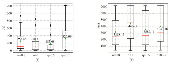
The results depicted in Figure 7 demonstrate that B&P is highly effective in solving large-sized problems with a tighter time limit of $A{G}_2$ or containing fewer $A{G}_1$ jobs. In the boxplots, red lines represent medians, green triangles denote mean values, and black circles indicate outliers. For example, in the first subfigure, when $\alpha =0.8$, the mean is 253.46 s and the median is around 100 s; for $q=0.5$, the mean is 183.68 s (median ~80 s), indicating lower time consumption. A larger $q$ (e.g., $q=0.75$, mean 320.09 s) or $\alpha =1$ (mean 250.31 s) leads to increased time in the first subfigure, while in the second subfigure, $\alpha =1$ (mean 4436.4 s) and $q=0.75$ (mean 4037.36 s) also show higher time than $\alpha =0.8$ (mean 3188.13 s) and $q=0.5$ (mean 3587.16 s). This confirms that a larger lead to smaller time consumption of B&P, as a smaller number of machines prevents efficient reduction of reduced cost in the pricing problem, causing repeated fluctuations. In summary, this study can efficiently satisfy the $A{G}_2$ due date and minimize the total weighted completion time of $A{G}_1$. Computational results demonstrate that the proposed B&P algorithm has excellent performance in both optimality and efficiency.

Figure 7. Summary of CPU time for large-sized instances: (a) box-plots of B&P; $t(s)$ in Table 7; (b) box-plots of B&P: $t(s)$ in Table 8.

6. Conclusions

This research addresses the problem of multitasking scheduling for two competitive agents on identical parallel machines, a challenge directly motivated by resource allocation in loud manufacturing (CMfg) platforms. The objective is to minimize the total weighted completion time of the first agent’s ($A{G}_1$) long-term tasks, subject to the constraint that the makespan of the second agent’s ($A{G}_2$) urgent tasks satisfies in a strict time limit. We established key structural properties and developed an exact branch-and-price (B&P) approach, enhanced by a two-phase label-setting algorithm and dominance rules. Computational experiments demonstrated that the B&P approach successfully solved 92.31% of instances and provided a robust solution for optimizing platform operations by efficiently balancing urgent and flexible task commitments.

Despite its effectiveness, the approach’s computational efficiency is challenged by very large-scale instances with tight due-date constraints, highlighting a limitation in scalability. From a managerial perspective, this model offers clear value to CMfg platforms by enabling efficient resource allocation. It guarantees urgent service deadlines without compromising the scheduling of long-term projects, thereby enhancing operational reliability and customer satisfaction.

For future work, promising directions include hybridizing the exact B&P algorithm with metaheuristics to improve scalability and extending the model to unrelated parallel machines to better handle heterogeneous manufacturing resources. Investigating the multi-objective problem that also minimizes the makespan of $A{G}_2$ presents another valuable research avenue.

References

- Yuan, C.; Wang, Y. Design and strategy selection for quality incentive mechanisms in the public cloud manufacturing model. Comput. Ind. Eng. 2024, 198, 110681. [Google Scholar] [CrossRef]
- Jiang, Y.; Tang, D.; Zhu, H.; Liu, C.; Chen, K.; Zhang, Z.; Chen, J. A skill vector-based multi-task optimization algorithm for achieving objectives of multiple users in cloud manufacturing. Adv. Eng. Inform. 2025, 65, 103295. [Google Scholar] [CrossRef]
- Wang, D.; Yu, Y.; Yin, Y.; Cheng, T.C.E. Multi-agent scheduling problems under multitasking. Int. J. Prod. Res. 2021, 59, 3633–3663. [Google Scholar] [CrossRef]
- Hall, N.G.; Leung, J.Y.T.; Li, C.-L. The effects of multitasking on operations scheduling. Prod. Oper. Manag. 2015, 24, 1248–1265. [Google Scholar] [CrossRef]
- Xu, S.; Hall, N.G. Fatigue, personnel scheduling and operations: Review and research opportunities. Eur. J. Oper. Res. 2021, 295, 807–822. [Google Scholar] [CrossRef]
- Xue, H.; Bai, D.; Shu, X.; Wang, L.; Chu, F.; Cai, G. A multitasking scheduling problem of emergency medical response in mass casualty incident. IISE Trans. 2025, 1–19. [Google Scholar] [CrossRef]
- Graham, R.; Lawler, E.; Lenstra, J.; Kan, A. Optimization and Approximation in Deterministic Sequencing and Scheduling: A Survey. Ann. Discrete Math. 1979, 5, 287–326. [Google Scholar] [CrossRef]
- Hall, N.G.; Leung, J.Y.T.; Li, C.-L. Multitasking via alternate and shared processing: Algorithms and complexity. Discrete Appl. Math. 2016, 208, 41–58. [Google Scholar] [CrossRef]
- Li, S.-S.; Chen, R.-X.; Tian, J. Multitasking scheduling problems with two competitive agents. Eng. Optim. 2020, 52, 1940–1956. [Google Scholar] [CrossRef]
- Wu, C.-C.; Azzouz, A.; Chen, J.-Y.; Xu, J.; Shen, W.-L.; Lu, L.; Ben Said, L.; Lin, W.-C. A two-agent one-machine multitasking scheduling problem solving by exact and metaheuristics. Complex Intell. Syst. 2022, 8, 199–212. [Google Scholar] [CrossRef]
- Yang, Y.; Yin, G.; Wang, C.; Yin, Y. Due date assignment and two-agent scheduling under multitasking environment. J. Comb. Optim. 2020, 44, 2207–2223. [Google Scholar] [CrossRef]
- Wang, Y.; Wang, J.-Q.; Yin, Y. Due date assignment and multitasking scheduling with deterioration effect and efficiency promotion. Comput. Ind. Eng. 2020, 146, 106569. [Google Scholar] [CrossRef]
- Lee, W.-C.; Wang, J.-Y.; Lin, M.-C. A branch-and-bound algorithm for minimizing the total weighted completion time on parallel identical machines with two competing agents. Knowl. Based Syst. 2016, 105, 68–82. [Google Scholar] [CrossRef]
- Xiong, X.; Zhou, P.; Yin, Y.; Cheng, T.C.E.; Li, D. An exact branch-and-price algorithm for multitasking scheduling on unrelated parallel machines. Nav. Res. Logist. 2019, 66, 502–516. [Google Scholar] [CrossRef]
- Gao, J.; Zhu, X.; Zhang, R. A branch-and-price approach to the multitasking scheduling with batch control on parallel machines. Int. Trans. Oper. Res. 2022, 29, 3464–3485. [Google Scholar] [CrossRef]
- Santos, F.; Fukasawa, R.; Ricardez-Sandoval, L. An integrated machine scheduling and personnel allocation problem for large-scale industrial facilities using a rolling horizon framework. Optim. Eng. 2021, 22, 2603–2626. [Google Scholar] [CrossRef]
- Zhu, Z.; Li, J.; Chu, C. Multitasking scheduling problems with deterioration effect. Math. Probl. Eng. 2017, 2017, 4750791. [Google Scholar] [CrossRef]
- Zhu, Z.; Zheng, F.; Chu, C. Multitasking scheduling problems with a rate-modifying activity. Int. J. Prod. Res. 2017, 55, 296–312. [Google Scholar] [CrossRef]
- Zhu, Z.; Liu, M.; Chu, C.; Li, J. Multitasking scheduling with multiple rate-modifying activities. Int. Trans. Oper. Res. 2019, 26, 1956–1976. [Google Scholar] [CrossRef]
- Ji, M.; Zhang, Y.; Zhang, Y.; Cheng, T.C.E.; Jiang, Y. Single-machine multitasking scheduling with job efficiency promotion. J. Comb. Optim. 2022, 44, 446–479. [Google Scholar] [CrossRef]
- Liu, M.; Wang, S.; Zheng, F.; Chu, C. Algorithms for the joint multitasking scheduling and common due year assignment problem. Int. J. Prod. Res. 2017, 55, 6052–6066. [Google Scholar] [CrossRef]
- Ji, M.; Zhang, W.; Liao, L.; Cheng, T.C.E.; Tan, Y. Multitasking parallel-machine scheduling with machine-dependent slack due-window assignment. Int. J. Prod. Res. 2019, 57, 1667–1684. [Google Scholar] [CrossRef]
- Xu, C.; Xu, Y.; Zheng, F.; Liu, M. Multitasking scheduling problems with a common due-window. RAIRO–Oper. Res. 2021, 55, 1787–1798. [Google Scholar] [CrossRef]
- Xu, X.; Yin, G.; Wang, C. Multitasking scheduling with batch distribution and due data assignment. Comput. Int. Syst. 2021, 7, 191–202. [Google Scholar] [CrossRef]
- Li, J.; Li, X.; Gao, L.; Wang, C.; Chen, H. A multitasking workforce-constrained flexible job shop scheduling problem: An application from a real-world workshop. J. Manuf. Syst. 2025, 83, 196–215. [Google Scholar] [CrossRef]
- Hu, M.; Zhang, W.; Ren, X.; Qin, S.; Chen, H.; Zhang, J. A novel resilient scheduling method based on multi-agent system for flexible job shops. Int. J. Prod. Res. 2025, 1–21. [Google Scholar] [CrossRef]
- Zhang, L.; Yan, Y.; Hu, Y. Dynamic flexible scheduling with transportation constraints by multi-agent reinforcement learning. Eng. Appl. Artif. Intell. 2024, 134, 108699. [Google Scholar] [CrossRef]
- Agnetis, A.; Mirchandani, P.B.; Pacciarelli, D.; Pacifici, A. Scheduling problems with two competing agents. Oper. Res. 2004, 52, 229–242. [Google Scholar] [CrossRef]
- Leung, J.Y.-T.; Pinedo, M.; Wan, G. Competitive two-agent scheduling and its applications. Oper. Res. 2010, 58, 458–469. [Google Scholar] [CrossRef]
- Gerstl, E.; Mosheiov, G. Scheduling problems with two competing agents to minimized weighted earliness-tardiness. Comput. Oper. Res. 2013, 40, 109–116. [Google Scholar] [CrossRef]
- Shabtay, D.; Dover, O.; Kaspi, M. Single-machine two-agent scheduling involving a just-in-time criterion. Int. J. Comput. Prod. Res. 2015, 53, 2590–2604. [Google Scholar] [CrossRef]
- Li, H.; Gajpal, Y.; Bector, C. Single machine scheduling with two-agent for total weighted completion time objectives. Appl. Soft Comput. 2018, 70, 147–156. [Google Scholar] [CrossRef]
- Zhang, X. Two competitive agents to minimize the weighted total late work and the total completion time. Appl. Math. Comput. 2021, 406, 126286. [Google Scholar] [CrossRef]
- Lin, W.-C.; Yin, Y.; Cheng, S.-R.; Cheng, T.; Wu, C.-H.; Wu, C.-C. Particle swarm optimization and opposite-based particle swarm optimization for two-agent multi-facility customer order scheduling with ready times. Appl. Soft Comput. 2017, 52, 877–884. [Google Scholar] [CrossRef]
- Choi, B.C.; Park, M.J. Two-agent parallel machine scheduling with a restricted number of overlapped reserved tasks. Eur. J. Oper. Res. 2017, 260, 514–519. [Google Scholar] [CrossRef]
- Smith, W.E. Various optimizers for single-stage production. Nav. Res. Logist. Q. 1956, 3, 59–66. [Google Scholar] [CrossRef]
- Bruno, J.; Coffman, E.G.; Sethi, R. Scheduling independent tasks to reduce mean finishing time. Commun. ACM 1974, 17, 382–387. [Google Scholar] [CrossRef]
- Chen, Z.-L.; Powell, W.B. Solving Parallel Machine Scheduling Problems by Column Generation. INFORMS J. Comput. 1999, 11, 78–94. [Google Scholar] [CrossRef]
- Kowalczyk, D.; Leus, R. A branch-and-price algorithm for parallel machine scheduling using ZDDs and generic branching. INFORMS J. Comput. 2018, 30, 768–782. [Google Scholar] [CrossRef]
- Kramer, A.; Dell’Amico, M.; Iori, M. Enhanced arc-flow formulations to minimize weighted completion time on identical parallel machines. Eur. J. Oper. Res. 2019, 275, 67–79. [Google Scholar] [CrossRef]
- Wang, C.; Guo, C.; Zuo, X. Solving multi-depot electric vehicle scheduling problem by column generation and genetic algorithm. Appl. Soft Comput. 2021, 112, 107774. [Google Scholar] [CrossRef]
- Gunawan, A.; Widjaja, A.T.; Vansteenwegen, P.; Yu, V.F. A matheuristic algorithm for the vehicle routing problem with cross-docking. Appl. Soft Comput. 2021, 103, 107163. [Google Scholar] [CrossRef]
- Gao, J.; Zhu, X.; Zhang, R. Scheduling for trial production with a parallel machine and multitasking scheduling model. Appl. Intell. 2023, 53, 26907–26926. [Google Scholar] [CrossRef]
- Azizoglu, M.; Kirca, O. On the minimization of total weighted Flow time with identical and uniform parallel machines. Eur. J. Oper. Res. 1999, 32, 91–100. [Google Scholar] [CrossRef]
- Elmaghraby, S.E.; Park, S.H. Scheduling jobs on a number of identical machines. AIIE Trans. 1974, 6, 1–13. [Google Scholar] [CrossRef]
- Muts, P.; Bruche, S.; Nowak, I.; Wu, O.; Hendrix, E.M.T.; Tsatsaronis, G. A column generation algorithm for solving energy system planning problems. Optim. Eng. 2023, 24, 317–351. [Google Scholar] [CrossRef]
- Jepsen, M.; Petersen, B.; Spoorendonk, S.; Pisinger, D. Subset-row inequalities applied to the vehicle-routing problem with time windows. Oper. Res. 2008, 56, 497–511. [Google Scholar] [CrossRef]
- Sedeño-Noda, A.; González-Martín, C. An efficient label setting/correcting shortest path algorithm. Comput. Optim. Appl. 2012, 51, 437–455. [Google Scholar] [CrossRef]
- Li, C.; Gong, L.; Luo, Z.; Lim, A. A branch-and-price-and-cut algorithm for a pickup and delivery problem in retailing. Omega 2019, 89, 71–91. [Google Scholar] [CrossRef]
- Muter, I. Exact algorithms to minimize makespan on single and parallel batch processing machines. Eur. J. Oper. Res. 2020, 285, 470–483. [Google Scholar] [CrossRef]
- Kramer, H.H.; Uchoa, E.; Fampa, M.; Köhler, V.; Vanderbeck, F. Column generation approaches for the software clustering problem. Comput. Optim. Appl. 2016, 64, 843–864. [Google Scholar] [CrossRef]
- van den Akker, J.M.; Hoogeveen, J.; van de Velde, A.S.L. Parallel Machine Scheduling by Column Generation. Oper. Res. 1999, 47, 862–872. [Google Scholar] [CrossRef]
- Dell’Amico, M.; Iori, M.; Martello, S.; Monaci, M. Heuristic and exact algorithms for the identical parallel machine scheduling problem. INFORMS J. Comput. 2008, 20, 333–344. [Google Scholar] [CrossRef]
Disclaimer/Publisher’s Note: The statements, opinions and data contained in all publications are solely those of the individual author(s) and contributor(s) and not of MDPI and/or the editor(s). MDPI and/or the editor(s) disclaim responsibility for any injury to people or property resulting from any ideas, methods, instructions or products referred to in the content. |
© 2025 by the authors. Licensee MDPI, Basel, Switzerland. This article is an open access article distributed under the terms and conditions of the Creative Commons Attribution (CC BY) license (https://creativecommons.org/licenses/by/4.0/).