Fleet Monitoring of Bridge Using Direct Calculation of Moving Reference Influence Line

Abstract

Bridges are critical components of transport networks, yet they inevitably deteriorate over time. Damage in a bridge reduces its stiffness, altering both its static and dynamic responses to loading. This change also affects the dynamic excitation of the loading source, such as a passing vehicle, meaning that vehicle vibrations can be used to infer bridge damage. Deflections under a moving instrumented axle are influenced by both bridge and vehicle properties, making them unique to each vehicle. To extract meaningful information about bridge conditions, these data must therefore be transformed into a form independent of vehicle characteristics. The bridge influence line, defined as the response to a unit moving load, provides a reliable descriptor of structural behaviour that is unaffected by vehicle properties. In this study, a fleet of vehicles is simulated to generate acceleration signals, from which bridge influence lines are derived using the inverse Newmark–beta method. Two damage indicators are proposed: D1, derived from the mid-span point of the mean Moving Reference Influence Line (MRIL), and D2, defined as the area under the mean MRIL curve. Results show that both indicators can effectively detect global bridge damage. D2 exhibits a clear linear relationship with stiffness loss and remains stable under varying speeds and noise levels, whereas D1 is more sensitive to factors such as measurement noise, vehicle speed, and variations in vehicle properties, but remains reliable at lower speeds and moderate noise levels. Measurement errors are simulated by adding random noise to the acceleration inputs, and the fleet monitoring approach is shown to mitigate these effects, enhancing the overall accuracy and robustness of bridge damage detection.

1. Introduction

Climate change, ageing infrastructure, and increasing traffic demand are placing growing pressure on transport networks worldwide [1]. Bridges, as critical nodes in these networks, are particularly vulnerable. Rising frequencies of extreme weather events such as flooding and heatwaves accelerate material deterioration, while chronic issues such as scour, corrosion, and fatigue further compromise structural integrity. In addition, widespread overloading of heavy goods vehicles has been reported across Europe and beyond, contributing to accelerated damage accumulation in bridge structures [2]. Ensuring the safety and serviceability of bridges under these combined challenges is therefore a matter of both economic and societal importance.

Structural Health Monitoring (SHM) has emerged as a powerful tool for assessing the condition of bridges in a systematic and data-driven manner [3]. Reliable SHM can reduce reliance on unscheduled maintenance, extend service life, and prevent catastrophic failures. Traditional approaches, however, remain limited. Visual inspections, though widely practiced, are subjective, labour-intensive, and sometimes unreliable, with damage often going undetected until it has reached an advanced stage [4]. More advanced vibration-based SHM techniques, which identify changes in modal properties such as frequency and mode shapes, have shown promise in laboratory and field studies [5]. Yet, these methods typically require expensive instrumentation installed directly on the bridge, extensive baseline data, and are often sensitive to environmental and operational variability, which complicates their application on a large scale.

In response to these limitations, alternative monitoring approaches have been explored in recent years. According to the European Commission’s Joint Research Centre reports [6], four key emerging directions in SHM have been identified: vision-based methods, satellite-based monitoring, UAV-based monitoring, and so-called “drive-by” monitoring [7]. Among these, drive-by monitoring has attracted considerable attention due to its scalability and cost-effectiveness. The principle is straightforward: inertial measurements collected from passing vehicles can provide indirect information on the bridge response [8]. A major advantage is that monitoring can be achieved opportunistically, using existing or specially instrumented vehicles, without the need for sensors on the bridge itself.

Since the seminal works of Yang et al. [9] and Yang and Lin [10], drive-by monitoring has developed into a vibrant research field. Studies have demonstrated its potential to extract bridge natural frequencies, damping, and even mode shapes from vehicle vibrations [11,12,13,14,15]. Other researchers have focused on damage detection without explicitly identifying modal properties. For instance, OBrien et al. [16] applied moving force identification to determine vehicle–bridge interaction forces, while OBrien and Keenahan [17] employed a traffic speed deflectometer vehicle model and cross-entropy optimisation to infer the apparent bridge profile. Li et al. [18] proposed a dual Kalman filter framework to first estimate road roughness and subsequently detect damage through sensitivity analysis. Collectively, these works demonstrate that drive-by monitoring is a promising indirect SHM technique, though challenges remain in terms of accuracy, robustness to noise, and dependency on vehicle properties.

A key challenge in drive-by bridge monitoring is that vehicle responses depend on both bridge and vehicle characteristics, making raw measurements unsuitable for direct assessment of bridge condition. To overcome this limitation, the MRIL concept is introduced. The MRIL, defined as the deflection at a moving reference point due to a unit load applied at a shifted location, provides a descriptor of bridge behaviour that is largely independent of vehicle properties. By focusing on MRILs, it becomes possible to separate structural effects from vehicle-specific influences, offering a more robust basis for bridge condition evaluation.

While several studies have explored vehicle-based monitoring using acceleration or strain responses, most approaches remain limited by dependence on vehicle characteristics or by the use of fixed-point influence lines [19,20,21]. The present work addresses these gaps by integrating the inverse Newmark–beta method with a fleet monitoring framework to estimate MRILs directly from vehicle acceleration signals. Furthermore, two novel damage indicators, based on the MRIL mid-span point and area, are developed and systematically assessed under multiple sources of uncertainty, including measurement noise, variability in vehicle properties, and speed effects. This study therefore contributes a new simulation-based framework that enhances the robustness and scalability of drive-by monitoring for bridge health assessment.

The remainder of this paper is structured as follows. Section 2 introduces the vehicle–bridge interaction model based on a quarter-car configuration. Section 3 presents the methodology, including the formulation of the proposed damage indicators. Section 4 reports and analyses the results under various uncertainty scenarios. Section 5 discusses key implications, modelling assumptions, and potential extensions, while Section 6 concludes the paper.

2. Vehicle–Bridge Interaction

To demonstrate the fleet monitoring concept for a bridge, a simple quarter-car and beam model with a smooth profile is simulated in MATLAB R2025b (Figure 1). A fleet of quarter-car vehicles is generated using the mean and standard deviation of vehicle properties listed in Table 1. The statistical parameters for typical truck fleet properties are adopted from Belay et al. [22]. The beam is modelled as simply supported using a finite element discretization. Vehicles are then simulated crossing the beam, and the corresponding acceleration responses are obtained. Vehicle–bridge coupling is introduced at the tyre contact points through the interaction force vector, and the coupled system is solved using the Newmark-beta integration scheme. For each simulation, deflections under the axle are reconstructed from the measured accelerations and vehicle properties using the inverse Newmark-beta method [23,24,25,26]. From these inferred deflections, MRILs are calculated for each vehicle.

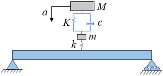
Figure 1. Quarter-car and bridge model.

Table 1. Vehicle properties.

Parameter	Symbol	Unit	Mean	St. Dev.
Sprung Mass	M	kg	4450	400
Unsprung Mass	m	kg	420	40
Suspension Stiffness	K	N/m	500,000	50,000
Tyre Stiffness	k	N/m	1,950,000	195,000
Suspension Damping	c	N·s/m	21,000	2000

In this study, a fleet of 50 vehicles is generated using Monte Carlo simulation with varying properties (Table 1). The bridge is represented as a 20 m span with a second moment of area of 0.33 m⁴, Young’s modulus of 35 × 10⁹ N/m², and a mass per unit length of 9.6 × 10³ kg/m, where the bridge properties are adopted from previous work on a typical T-beam bridge designed in accordance with British Standards, as reported in the literature [27]. The process is repeated for four bridge states, using the same batch of vehicles in each case. Each state corresponds to a different level of global damage, reflected in variations in MRILs. While load-carrying capacity is not identical to flexural rigidity (stiffness), the two are closely correlated; here, reductions in flexural rigidity are adopted as indicators of bridge deterioration. The levels of stiffness reduction considered are 0%, 5%, 10%, and 20%.

3. Methodology

3.1. Inverse Newmark-Beta Method for Calculating Bridge Influence Lines

The inverse Newmark–beta method is a modified application of the classical Newmark–beta integration scheme. While the conventional approach predicts accelerations, velocities, and displacements from a known excitation, the inverse formulation operates in reverse: it utilises measured vehicle accelerations together with known mechanical properties to reconstruct the corresponding bridge displacements beneath the moving vehicle. This allows the structural response to be recovered without requiring direct information on the road or track surface. When the surface profile is perfectly smooth, the apparent deflection obtained through this inverse process coincides with the actual bridge deflection. Consequently, the method offers an efficient means of extracting bridge condition information from vehicle-based measurements.

The MRIL further extends this concept by representing the bridge response, such as deflection, measured at a moving reference point (for instance, directly beneath a travelling axle) rather than at a fixed position on the structure. In contrast to conventional influence lines that describe the response at a static point under a unit moving load, the MRIL captures the coupled interaction between the bridge and the moving vehicle, providing a more realistic characterisation of bridge dynamics under vehicular excitation. A detailed description of the MRIL formulation can be found in previous work [26].

3.2. Damage Indicator

Figure 2 presents the calculated MRILs for all vehicles and four bridge conditions, namely the healthy, 5% damaged, 10% damaged, and 20% damaged states. As shown in Figure 2a, the MRILs obtained from 50 simulated vehicle passages display consistent patterns across all bridge conditions, with the magnitude of the MRIL increasing progressively as the damage level rises. Figure 2b illustrates the MRILs from the healthy bridge case, confirming the good repeatability among different vehicle runs and demonstrating the robustness of the moving reference approach regarding various vehicle properties, as stated in Table 1. The averaged results for the 50 vehicles are plotted in Figure 2c, where the mean MRILs show a clear and smooth distribution. The MRIL amplitude ranges approximately from 0 to 6 × 10⁻⁸ m/kN, and a noticeable upward shift is observed as the damage severity increases, indicating that the structural stiffness reduction has a measurable influence on the bridge’s dynamic response captured by the MRILs.

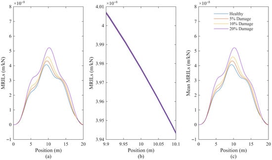
Figure 2. MRILs under four bridge conditions: healthy, 5%, 10%, and 20% damaged. (a) MRILs from 50 vehicles, (b) healthy case showing repeatability, and (c) mean MRILs for each damage level.

The mid-span point of the mean of the 50 MRIL curves, denoted as $\widetilde{\mathrm{M}\mathrm{R}\mathrm{I}\mathrm{L}}$, is selected as damage indicator 1 (D1), as defined in Equation (1). Here, ${\displaystyle \raisebox{1ex}{$1$}\!\left/ \!\raisebox{-1ex}{$\widetilde{\mathrm{M}\mathrm{R}\mathrm{I}\mathrm{L}}$}\right.}$ represents the inverse of the mean MRIL mid-span value. Physically, when the bridge loses stiffness (i.e., lower $EI$), its deflection under a unit moving load increases. Therefore, the MRIL amplitude or mid-span value becomes larger as stiffness decreases. Consequently, a reduction in stiffness corresponds to larger MRIL mid-span values and, equivalently, smaller inverse values ${\displaystyle \raisebox{1ex}{$1$}\!\left/ \!\raisebox{-1ex}{$\widetilde{\mathrm{M}\mathrm{R}\mathrm{I}\mathrm{L}}$}\right.}$. The superscripts D and H denote the damaged and healthy bridge states, respectively. Accordingly, D1 decreases as bridge stiffness is reduced, providing an indirect but effective measure of structural damage [26]. As an alternative, damage indicator 2 (D2) is defined as the area under the mean MRIL curve, denoted as ${\mathrm{M}\mathrm{R}\mathrm{I}\mathrm{L}}^{\mathrm{*}}$, as shown in Equation (2). Unlike D1, which is derived from a single mid-span point, D2 considers the entire mean MRIL curve, making it more stable and representative of the overall structural behaviour.

$$\begin{array}{c}D1=100\times \left\{1-{\displaystyle \frac{{\left(\raisebox{1ex}{$1$}\!\left/ \!\raisebox{-1ex}{$\widetilde{\mathrm{M}\mathrm{R}\mathrm{I}\mathrm{L}}$}\right.\right)}^{\mathrm{D}}}{{\left(\raisebox{1ex}{$1$}\!\left/ \!\raisebox{-1ex}{$\widetilde{\mathrm{M}\mathrm{R}\mathrm{I}\mathrm{L}}$}\right.\right)}^{\mathrm{H}}}}\right\}=100\times \left\{1-{\displaystyle \frac{{\left(\widetilde{\mathrm{M}\mathrm{R}\mathrm{I}\mathrm{L}}\right)}^{\mathrm{H}}}{{\left(\widetilde{\mathrm{M}\mathrm{R}\mathrm{I}\mathrm{L}}\right)}^{\mathrm{D}}}}\right\}\end{array}$$

(1)

$$\begin{array}{c}D2=100\times \left\{1-{\displaystyle \frac{{\left(\raisebox{1ex}{$1$}\!\left/ \!\raisebox{-1ex}{${\mathrm{M}\mathrm{R}\mathrm{I}\mathrm{L}}^{\mathrm{*}}$}\right.\right)}^{\mathrm{D}}}{{\left(\raisebox{1ex}{$1$}\!\left/ \!\raisebox{-1ex}{${\mathrm{M}\mathrm{R}\mathrm{I}\mathrm{L}}^{\mathrm{*}}$}\right.\right)}^{\mathrm{H}}}}\right\}=100\times \left\{1-{\displaystyle \frac{{\left({\mathrm{M}\mathrm{R}\mathrm{I}\mathrm{L}}^{\mathrm{*}}\right)}^{\mathrm{H}}}{{{(\mathrm{M}\mathrm{R}\mathrm{I}\mathrm{L}}^{\mathrm{*}})}^{\mathrm{D}}}}\right\}\end{array}$$

(2)

The calculated damage indicator values are presented in Table 2. Both indicators show a clear correlation with the true damage levels. Damage indicator D2 exhibits a perfectly proportional relationship, reproducing the true values exactly (5%, 10%, and 20%), which highlights its potential as a linear measure of stiffness loss. In contrast, damage indicator D1 consistently overestimates the damage level: for example, at 10% true damage, damage indicator D1 yields 13%, and at 20% true damage, it predicts 24%. While this lack of direct proportionality may be a limitation, damage indicator D1 still captures the overall trend in structural deterioration.

Table 2. Inferred damaged indicators and true damage levels (D1 and D2 defined in Equations (1) and (2)).

True Damage Level	0%	5%	10%	20%
D1	0%	7%	13%	24%
D2	0%	5%	10%	20%

These results indicate that both indicators are capable of detecting bridge damage. Damage indicator D2, which integrates the entire MRIL, exhibits a clear linear relationship with stiffness reduction. In contrast, damage indicator D1, derived from a single point of the MRIL, is more sensitive to parameters such as vehicle speed, mechanical properties, and measurement noise, and therefore tends to slightly overestimate or underestimate the overall damage level. In this initial example, the analysis assumes all vehicles travel at a constant speed of 80 km/h and that their properties are perfectly known, allowing the fundamental performance of the indicators to be assessed under ideal conditions.

4. Results

4.1. Sensitivity to Measurement Noise

To evaluate the robustness of the method against measurement inaccuracies, random noise levels of 2% and 5% were added to the simulated acceleration signals. The calculated MRILs for all 50 vehicles and four bridge conditions (healthy, 5%, 10%, and 20% damaged) are presented in Figure 3 and Figure 4, corresponding to 2% and 5% noise levels, respectively.

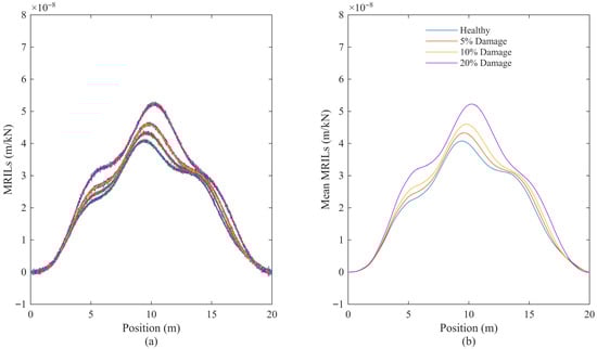
Figure 3. Calculated MRILs with 2% measurement noise for four bridge conditions: healthy, 5%, 10%, and 20% damaged. (a) MRILs from all 50 vehicles; (b) corresponding mean MRILs.

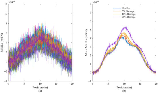
Figure 4. Calculated MRILs with 5% measurement noise for four bridge conditions: healthy, 5%, 10%, and 20% damaged. (a) MRILs from all 50 vehicles; (b) corresponding mean MRILs.

As shown in Figure 3a, the MRILs under 2% noise maintain smooth and consistent profiles across all vehicles, with only slight variations. The mean MRILs in Figure 3b closely match the noise-free results, confirming that averaging across vehicles effectively reduces random disturbances and preserves the overall shape.

When the noise level increases to 5% (Figure 4), the individual MRILs in Figure 4a become more scattered, indicating a stronger noise influence on the raw acceleration data. Nevertheless, the mean MRILs in Figure 4b still exhibit characteristic patterns and relative differences among damage levels. Although higher noise introduces visible fluctuations, the average MRILs remain stable enough to distinguish between bridge conditions, demonstrating the method’s resilience to moderate measurement noise.

The performance of the damage indicators is summarised in Table 3. Both indicators are capable of detecting stiffness loss and distinguishing between different damage states, even in the presence of measurement noise. However, their behaviours differ noticeably. Damage indicator D2, which accounts for the entire MRIL curve, exhibits a clear and nearly linear relationship with the true damage levels, increasing proportionally with stiffness reduction and maintaining stability across all noise conditions. In contrast, damage indicator D1, derived from a single point on the MRIL, shows greater variability and tends to slightly overestimate damage, particularly under higher noise levels. Although damage indicator D1 still captures the correct progression of damage, its sensitivity to measurement noise limits its reliability compared with damage indicator D2.

Table 3. Inferred damaged indicators and true damage levels.

Damage Indicator	Noise	True Damage Level
		0%	5%	10%	20%
D1	0%	0%	7%	13%	24%
	2%	0%	7%	13%	24%
	5%	0%	5%	12%	23%
D2	0%	0%	5%	10%	20%
	2%	0%	5%	10%	20%
	5%	0%	7%	10%	18%

Overall, these results demonstrate that damage indicator D2 provides a more robust and proportional estimate of global stiffness reduction, while damage indicator D1 may serve as a supplementary indicator under moderate noise conditions. The findings reinforce that the area-based damage indicator D2 formulation offers superior consistency and is better suited for practical bridge damage assessment.

4.2. Sensitivity to Vehicle Properties

Botshekan et al. reported that truck vehicle properties can vary by up to 40%, particularly in tyre and suspension stiffness, across different truck types [28]. Similarly, in practical traffic conditions, vehicle dynamic properties are inherently uncertain due to factors such as ageing, tyre wear, tyre pressure, and manufacturing or model-generation differences, all of which can introduce variability and potential errors in MRIL estimation. To investigate this effect, a 10% random variability was applied to all vehicle parameters, including mass, stiffness, and damping. The true and perturbed vehicle properties for the simulated fleet are shown in Figure 5, while the corresponding MRILs are presented in Figure 6.

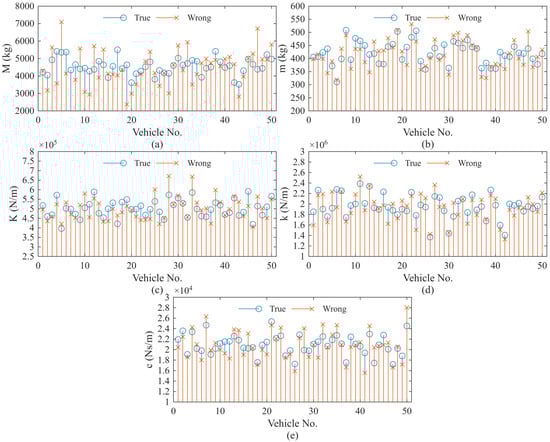
Figure 5. True and perturbed vehicle parameters with 10% random variability for the simulated fleet: (a) sprung mass, (b) unsprung mass, (c) suspension stiffness, (d) tyre stiffness, and (e) suspension damping.

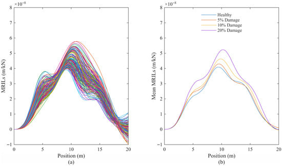
Figure 6. MRILs calculated with perturbed vehicle parameters: (a) all 50 vehicles showing strong variability; (b) mean MRILs for four bridge conditions (healthy, 5%, 10%, 20% damaged).

As illustrated in Figure 5, the randomly perturbed vehicle parameters deviate notably from their true values, introducing variability in the moving reference input data. This uncertainty directly affects the accuracy of the calculated MRILs. In Figure 6a, the MRILs derived using the incorrect vehicle properties display significant scatter and distorted profiles, making it difficult to identify bridge conditions from individual runs. However, the averaged MRILs shown in Figure 6b successfully recover the characteristic shapes observed in the reference case and remain responsive to the level of structural damage.

These findings suggest that while inaccurate vehicle parameters can considerably distort single-vehicle MRILs, ensemble averaging across multiple vehicles effectively mitigates the influence of parameter uncertainty and preserves sensitivity to bridge stiffness variations.

The mean values of the damage indicators are summarised in Table 4. Both indicators continue to capture the overall damage progression, albeit with slightly reduced accuracy compared with the noise-only case. For instance, at a true damage level of 5%, damage indicator D1 reproduces the value almost exactly (5%), whereas damage indicator D2 slightly underestimates it (2%). At higher damage levels, both indicators tend to overpredict marginally; for a true damage of 20%, damage indicator D1 gives 23%, and damage indicator D2 yields 20%. These results indicate that variability in vehicle properties introduces some loss of precision, yet both indicators still provide a reliable representation of the underlying structural condition. Damage indicator D1 appears marginally more accurate in this scenario, while damage indicator D2 maintains good consistency across the entire damage range.

Table 4. Inferred damaged indicators and true damage levels with wrong properties.

True Damage Level	0%	5%	10%	20%
D1	0%	5%	13%	23%
D2	0%	2%	11%	20%

Overall, these findings emphasise the importance of accounting for uncertainty in vehicle parameters. Although such variability affects the accuracy of the inferred damage estimates, the fleet-averaging approach effectively mitigates its influence, ensuring that the dominant damage trend remains clearly identifiable.

4.3. Sensitivity to Vehicle Speeds

Vehicle speed has a direct influence on the dynamic interaction between the vehicle and the bridge, thereby affecting the oscillatory behaviour of the calculated MRILs. To examine this effect, two extreme speed conditions were considered: a high speed of 120 km/h and a low speed of 10 km/h. The MRILs obtained from all vehicles under these two scenarios are shown in Figure 7 and Figure 8, respectively.

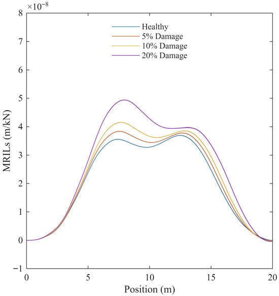
Figure 7. Calculated MRILs for four bridge conditions (healthy, 5%, 10%, and 20% damaged) at a vehicle speed of 120 km/h.

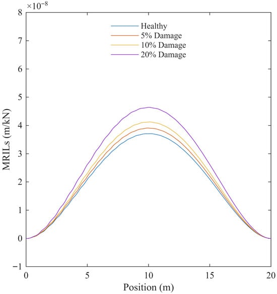
Figure 8. Calculated MRILs for four bridge conditions (healthy, 5%, 10%, and 20% damaged) at a vehicle speed of 10 km/h.

At high speed (Figure 7), the MRILs display a slightly smoother shape with reduced local oscillations, as the shorter interaction time between the vehicle and the bridge limits the number of vibration cycles excited by each vehicle. Nevertheless, the overall trends and sensitivity to damage remain clearly observable.

In contrast, at low speed (Figure 8), the MRILs exhibit a broader response with increased amplitude near mid-span, reflecting stronger dynamic coupling and more pronounced bridge deflections. The influence of damage is again evident, with the amplitude of the MRILs increasing systematically as the damage level rises.

These observations confirm that while vehicle speed affects the detailed profile of the MRILs, the overall shape and their ability to differentiate between bridge conditions remain consistent, demonstrating the robustness of the approach across a wide range of operating speeds.

The corresponding damage indicator values are summarised in Table 5. The results show that although higher vehicle speeds amplify the dynamic vehicle–bridge interaction and introduce additional oscillations in the influence lines, both indicators effectively capture the progression of bridge deterioration. At the higher speed of 120 km/h, damage indicator D1 slightly overestimates the damage, reporting 23% for a true 20% stiffness loss, while damage indicator D2 yields a comparable result of 21%. In contrast, at the lower speed of 10 km/h, both indicators closely match the true damage, each predicting 20% for the 20% damage case.

Table 5. Inferred damaged indicators and true damage levels for different vehicle speeds.

Damage Indicator	Speed km/h	True Damage Level
		0%	5%	10%	20%
D1	120	0%	5%	10%	23%
	10	0%	5%	10%	20%
D2	120	0%	5%	11%	21%
	10	0%	5%	10%	20%

These results indicate that lower speeds lead to smoother influence lines and more accurate indicator estimates, as dynamic effects are minimised. Overall, while higher speeds introduce greater variability, both indicators—particularly damage indicator D2—remain capable of reliably identifying damage levels. The findings highlight that vehicle speed plays a critical role in the accuracy and stability of the fleet-based monitoring approach.

Figure 9 illustrates the relationship between vehicle speed and the two proposed damage indicators, D1 and D2, for vehicle speeds ranging from 80 to 100 km/h, which represent typical fleet speeds on highways. Both indicators maintain values close to 0.1, consistent with the actual global stiffness reduction of 10%. This confirms that both D1 and D2 correctly capture the bridge damage level under varying speeds.

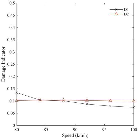
Figure 9. Variation in damage indicators D1 and D2 with vehicle speed (80–100 km/h) for a bridge with 10% damage.

However, a distinct difference in stability is observed between the two indicators. The black curve (D1), which is based on the mid-span magnitude of the MRIL, shows greater variability with various speeds. This sensitivity arises because D1 depends on a single point in the MRIL curve, which is more affected by local fluctuations and dynamic vehicle–bridge interaction effects. In contrast, the red curve (D2), derived from the area under the MRIL curve, remains nearly constant across all tested speeds. Since D2 integrates the full MRIL curve, it averages out local variations and is therefore more robust against speed-induced dynamic effects.

Overall, these results demonstrate that damage indicator D2 provides a more stable and reliable measure of stiffness reduction across a realistic range of highway speeds, while damage indicator D1 remains useful but less consistent at higher speeds. The continuous trend presented here complements the previous discrete speed analyses (10, 80, 120 km/h) and confirms that vehicle speed has only a minor effect on the overall accuracy of the fleet-based damage detection approach.

4.4. Combined Sensitivity Analysis

Finally, the combined effects of measurement noise and vehicle parameter variability were examined under three different speed conditions. Simulations were conducted at 120 km/h, 80 km/h, and 10 km/h, and the corresponding MRILs for all vehicles, together with their mean values, are presented in Figure 10, Figure 11 and Figure 12, respectively.

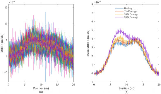
Figure 10. MRILs calculated under combined noise and vehicle parameter variability at a speed of 120 km/h for four bridge conditions (healthy, 5%, 10%, 20% damaged): (a) all vehicles; (b) mean MRILs.

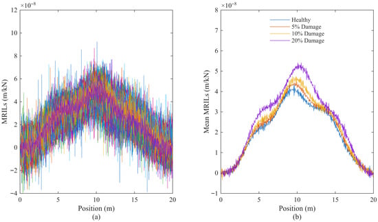
Figure 11. MRILs calculated under combined noise and vehicle parameter variability at a speed of 80 km/h for four bridge conditions (healthy, 5%, 10%, 20% damaged): (a) all vehicles; (b) mean MRILs.

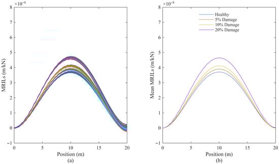
Figure 12. MRILs calculated under combined noise and vehicle parameter variability at a speed of 10 km/h for four bridge conditions (healthy, 5%, 10%, 20% damaged): (a) all vehicles; (b) mean MRILs.

As expected, the individual MRILs exhibit pronounced fluctuations due to the simultaneous influence of noise and uncertain vehicle parameters, particularly at higher speeds. Under these conditions, the individual results fail to provide a reliable indication of bridge conditions. However, after averaging across the fleet, the mean MRILs consistently reproduce the expected patterns and retain clear distinctions among the different damage levels.

The results further demonstrate that lower vehicle speeds yield smoother and more stable MRILs, as dynamic effects are reduced and the excitation becomes more quasi-static. Moreover, considering that the legal speed limit for heavy trucks in Europe typically lies below 120 km/h, the medium- and low-speed cases (80 km/h and 10 km/h) provide more realistic representations of practical traffic scenarios.

Overall, the findings confirm that the proposed MRIL-based approach remains effective under combined sources of uncertainty, particularly when a sufficient number of vehicle passages are considered for averaging.

The calculated damage levels are summarised in Table 6. At the highest speed of 120 km/h, damage indicator D1 performs less reliably, even yielding negative values at low damage levels (−8% and −5% for the 5% and 10% true damage cases, respectively). These negative values arise because the extracted mid-span MRIL amplitudes for the 5% and 10% damaged bridges become slightly smaller than that of the healthy bridge, leading to negative ratios when applying Equation (1). This behaviour reflects D1’s heightened sensitivity to noise and dynamic vehicle–bridge interaction effects under high-speed conditions, rather than indicating numerical instability. In contrast, damage indicator D2 remains stable, producing 10% and 16% for the same cases, although it still exhibits a slight tendency to overestimate the true damage. At a moderate speed of 80 km/h, the results improve, that damage indicator D1 slightly underestimates at 5% (2%) and marginally overestimates at 20% (22%), while damage indicator D2 remains closer to the true values, ranging from 8% at 5% damage to 21% at 20% damage. At the lowest speed of 10 km/h, both indicators show strong agreement with the true damage levels, with D1 and D2 accurately reproducing the 5%, 10%, and 20% cases with minimal deviation.

Table 6. Inferred damaged indicators and true damage levels for different speeds.

Damage Indicator	Speed km/h	True Damage Level
		0%	5%	10%	20%
D1	120	0%	−8%	−5%	15%
	80	0%	2%	10%	22%
	10	0%	5%	10%	20%
D2	120	0%	10%	16%	24%
	80	0%	8%	15%	21%
	10	0%	5%	10%	20%

Overall, these results demonstrate that the combined effects of measurement noise and variability in vehicle properties reduce the reliability of the inferred damage levels, particularly at higher speeds. However, the use of fleet averaging and lower operating speeds effectively mitigates these effects. Damage indicator D2 proves more robust across all scenarios, whereas damage indicator D1 achieves comparable accuracy only when dynamic effects are reduced at lower speeds.

5. Discussions

Vehicle–Bridge Interaction Modelling: The proposed fleet monitoring framework, which integrates the inverse Newmark–beta method with MRILs, demonstrates strong potential for indirect or drive-by bridge damage detection. In this study, a QC model was adopted to represent vehicle–bridge interaction. This classical model effectively captures the essential dynamic coupling mechanisms and allows for clear physical interpretation of the MRIL-based damage detection process. However, it does not fully replicate the behaviour of real vehicles, such as multi-axle configurations, nonlinear suspension effects, or distributed loads. Future research should therefore extend the framework to more advanced vehicle–bridge interaction models to improve physical realism and applicability.

MRIL Characteristics and Advantages: The MRIL formulation differs fundamentally from the conventional influence line, which describes the bridge response at a fixed location to a unit moving load. In contrast, the MRIL defines the response at a moving reference point that travels with the instrumented vehicle axle. This formulation enables the reconstruction of bridge behaviour independent of specific vehicle properties. Moreover, averaging MRILs across a vehicle fleet further reduces variability arising from differences in vehicle mass, suspension stiffness, and damping, thereby improving robustness against vehicle heterogeneity.

Damage Indicators: Sensitivity and Performance: Two complementary damage indicators were introduced: D1, based on the mid-span value of the mean MRIL, and D2, based on the area under the mean MRIL curve. Because D1 depends on a single point, it is inherently more sensitive to local fluctuations and dynamic effects, particularly at higher speeds, sometimes leading to over- or underestimation of the actual damage level. By contrast, D2, which integrates the full MRIL curve, provides a smoother, more stable response and exhibits a nearly linear relationship with stiffness reduction. Figure 9 confirms that D2 maintains consistent performance under varying noise and speed conditions, whereas D1 performs best under lower-speed, moderate-noise scenarios.

Computational Cost and Scalability: The computational demand of the proposed framework depends primarily on the complexity of the bridge model and the size of the simulated fleet. Using a simplified beam–vehicle system, the computational cost in this study remained modest. In practical implementation, the approach is expected to be cost-efficient since it does not require any permanent on-bridge sensors—data can be collected passively from vehicles during normal operation. The scalability of the framework depends on fleet composition. Homogeneous fleets (e.g., public buses or heavy trucks with similar configurations) yield more consistent MRILs and enhance detection reliability. For heterogeneous fleets, calibration procedures or vehicle-specific correction factors may be required to maintain accuracy.

Influence of Road Surface and Traffic Conditions: Road surface roughness can affect the vehicle response and, consequently, MRIL estimation. This influence can be mitigated by comparing vehicle crossings at different speeds or using data from multiple axles (e.g., front and rear) to isolate bridge-induced responses from surface-induced effects. Under mixed-traffic conditions, the method is most effective for short- to medium-span bridges, where typically only one vehicle is present at a time. For longer spans, multiple vehicles may occupy the bridge simultaneously, increasing excitation but complicating the separation of individual effects. Future developments should explore advanced signal-processing techniques capable of distinguishing overlapping vehicle responses.

6. Conclusions

This study has investigated the use of fleet monitoring and the inverse Newmark–beta method for bridge damage detection through MRILs. A quarter-car model traversing a simply supported beam was employed to simulate a fleet of vehicles under various bridge conditions. Two damage indicators, based on the mid-span magnitude and the area under the mean MRIL, were proposed and examined under multiple sources of uncertainty, including measurement noise, variability in vehicle properties, and changes in vehicle speed.

The results demonstrate that both indicators can successfully detect bridge damage trends associated with global stiffness reduction. Damage indicator D2, which considers the entire MRIL curve, exhibits a clear linear relationship with stiffness loss, whereas damage indicator D1, derived from a single mid-span value of the MRIL, is more sensitive to measurement noise and variations in vehicle speed and properties. Fleet averaging proved particularly effective in mitigating the adverse effects of measurement noise and variability in vehicle properties, enabling the correct MRIL shape to be maintained. Vehicle speed was also found to influence the accuracy of the indicators: although high speeds introduced oscillations due to dynamic vehicle–bridge interaction, both indicators remained capable of identifying damage. At lower speeds, the MRILs were smoother, and the estimated damage levels were closer to the true values. The combined sensitivity analysis confirmed that uncertainty degrades accuracy at higher speeds, with damage indicator D2 remaining the more stable overall, and damage indicator D1 performing reliably when dynamic effects are minimised.

Despite these promising findings, several limitations remain. The study utilised a simplified quarter-car–beam model with global stiffness reductions, which does not capture the full complexity of real bridges or the effects of localised damage. Road surface roughness was not considered, and the assumption of a perfectly smooth profile represents an idealisation. Moreover, the framework relies on prior knowledge of vehicle properties, which in practice may be uncertain or unavailable. Finally, only simulated data were used, and the influence of real-world factors such as sensor noise, environmental variations, and mixed traffic conditions has yet to be evaluated.

Future research will focus on addressing the current limitations and advancing the proposed MRIL-based framework toward real-world implementation. A key priority will be the experimental and field validation of the method using data collected from actual vehicle–bridge interactions. This will involve (i) estimating vehicle dynamic properties through calibration runs or onboard measurements, (ii) mitigating road surface roughness effects using subtraction-based techniques (e.g., multi-speed or multi-axle comparisons), and (iii) applying the inverse Newmark–beta method to reconstruct MRILs from field data for evaluating the proposed damage indicators D1 and D2 under realistic operational conditions. In addition, future studies will explore more sophisticated vehicle–bridge interaction models [29], incorporating localised damage and nonlinear dynamics to improve physical realism. The explicit inclusion of road roughness and the development of adaptive algorithms to estimate or correct for unknown vehicle parameters will further enhance the robustness and practicality of the approach. Extending the framework to heterogeneous traffic environments and optimising fleet composition will help assess its scalability and performance under mixed traffic scenarios. Ultimately, integrating fleet-based monitoring with complementary sensing technologies, both indirect (e.g., drive-by methods) and direct (e.g., on-bridge instrumentation), is expected to lead to a scalable, cost-effective, and data-rich solution for large-scale bridge structural health monitoring.

References

- Rattanachot, W.; Wang, Y.; Chong, D.; Suwansawas, S. Adaptation strategies of transport infrastructures to global climate change. Transp. Policy 2015, 41, 159–166. [Google Scholar] [CrossRef]
- Jensen, J.S.; Frangopol, D.M.; Schmidt, J.W. Bridge Maintenance, Safety, Management, Digitalization and Sustainability; Taylor & Francis Group: London, UK, 2024. [Google Scholar] [CrossRef]
- Azimi, M.; Eslamlou, A.D.; Pekcan, G. Data-driven structural health monitoring and damage detection through deep learning: State-of-the-art review. Sensors 2020, 20, 2778. [Google Scholar] [CrossRef] [PubMed]
- Katam, R.; Pasupuleti, V.D.K.; Kalapatapu, P. A review on structural health monitoring: Past to present. Innov. Infrastruct. Solut. 2023, 8, 248. [Google Scholar] [CrossRef]
- Das, S.; Saha, P.; Patro, S.K. Vibration-based damage detection techniques used for health monitoring of structures: A review. J. Civ. Struct. Health Monit. 2016, 6, 477–507. [Google Scholar] [CrossRef]
- Gkoumas, K.; Stepniak, M.; Cheimariotis, I.; Marques dos Santos, F. New technologies for bridge inspection and monitoring: A perspective from European Union research and innovation projects. Struct. Infrastruct. Eng. 2024, 20, 1120–1132. [Google Scholar] [CrossRef]
- Elhattab, A.; Uddin, N.; OBrien, E.J. Drive-by bridge damage monitoring using Bridge Displacement Profile Difference. J. Civ. Struct. Health Monit. 2016, 6, 839–850. [Google Scholar] [CrossRef]
- McGetrick, P.J.; Kim, C.W.; González, A.; OBrien, E.J. Experimental validation of a drive-by stiffness identification method for bridge monitoring. Struct. Health Monit. 2015, 14, 317–331. [Google Scholar] [CrossRef]
- Yang, Y.B.; Lin, C.W.; Yau, J.D. Extracting bridge frequencies from the dynamic response of a passing vehicle. J. Sound Vib. 2004, 272, 471–493. [Google Scholar] [CrossRef]
- Yang, Y.B.; Lin, C.W. Vehicle–bridge interaction dynamics and potential applications. J. Sound Vib. 2005, 284, 205–226. [Google Scholar] [CrossRef]
- Malekjafarian, A.; McGetrick, P.J.; OBrien, E.J. A review of indirect bridge monitoring using passing vehicles. Shock Vib. 2015, 2015, 286139. [Google Scholar] [CrossRef]
- Yang, Y.B.; Wang, Z.L.; Shi, K.; Xu, H.; Wu, Y.T. State-of-the-art of vehicle-based methods for detecting various properties of highway bridges and railway tracks. Int. J. Struct. Stab. Dyn. 2020, 20, 2041004. [Google Scholar] [CrossRef]
- González, A.; OBrien, E.J.; McGetrick, P.J. Identification of damping in a bridge using a moving instrumented vehicle. J. Sound Vib. 2012, 331, 4115–4131. [Google Scholar] [CrossRef]
- Zhang, Y.; Wang, L.Q.; Xiang, Z.H. Damage detection by mode shape squares extracted from a passing vehicle. J. Sound Vib. 2012, 331, 291–307. [Google Scholar] [CrossRef]
- Li, Z.K.; Lin, W.W.; Zhang, Y. Drive-by bridge damage detection using Mel-frequency cepstral coefficients and support vector machine. Struct. Health Monit. 2023, 22, 3302–3319. [Google Scholar] [CrossRef]
- OBrien, E.J.; McGetrick, P.J.; González, A. A drive-by inspection system via vehicle moving force identification. Smart Struct. Syst. 2014, 13, 821–848. [Google Scholar] [CrossRef]
- OBrien, E.J.; Keenahan, J. Drive-by damage detection in bridges using the apparent profile. Struct. Control Health Monit. 2015, 22, 813–825. [Google Scholar] [CrossRef]
- Li, J.T.; Zhu, X.Q.; Law, S.S.; Samali, B. A two-step drive-by bridge damage detection using dual Kalman filter. Int. J. Struct. Stab. Dyn. 2020, 20, 2042006. [Google Scholar] [CrossRef]
- Liu, C.; Zhu, Y.; Zeng, Q.; Pan, C.; Duan, Z. Bridge damage identification using rotation influence line under random vehicle loads. Int. J. Struct. Stab. Dyn. 2024, 24, 2450085. [Google Scholar] [CrossRef]
- Wang, S.; Huseynov, F.; Casero, M.; OBrien, E.J.; Fidler, P.; McCrum, D.P. A novel bridge damage detection method based on the equivalent influence lines–Theoretical basis and field validation. Mech. Syst. Signal Process. 2023, 204, 110738. [Google Scholar] [CrossRef]
- Zheng, X.; Yi, T.H.; Yang, D.H.; Li, H.N. Stiffness estimation of girder bridges using influence lines identified from vehicle-induced structural responses. J. Eng. Mech. 2021, 147, 04021042. [Google Scholar] [CrossRef]
- Belay, A.; OBrien, E.J.; Kroese, D. Truck fleet model for design and assessment of flexible pavements. J. Sound Vib. 2008, 311, 1161–1174. [Google Scholar] [CrossRef]
- Keenahan, J.; Ren, Y.F.; OBrien, E.J. Determination of road profile using multiple passing vehicle measurements. Struct. Infrastruct. Eng. 2020, 16, 1262–1275. [Google Scholar] [CrossRef]
- Ren, Y.F.; OBrien, E.J.; Cantero, D.; Keenahan, J. Railway bridge condition monitoring using numerically calculated responses from batches of trains. Appl. Sci. 2022, 12, 4972. [Google Scholar] [CrossRef]
- OBrien, E.J.; Wilson, S.; Keenahan, J.; Ren, Y.F. A Bayesian approach to the estimation of road profile and bridge damage from a fleet passing vehicle measurements. Int. J. Struct. Stab. Dyn. 2024, 24, 2450040. [Google Scholar] [CrossRef]
- Ren, Y.F.; Feng, K.; OBrien, E.J.; Li, W.H.; He, H.F. Bridge Profile and Vehicle Property Determination Using Vehicle Fleet Monitoring Concept. Int. J. Struct. Stab. Dyn. 2024, 25, 2550219. [Google Scholar] [CrossRef]
- Li, Y.Y. Factors Affecting the Dynamic Interaction of Bridges and Vehicle Loads. Ph.D. Thesis, University College Dublin, Dublin, Ireland, 2006. Volume 9741. Available online: https://ucd.summon.serialssolutions.com/?formids=target&lang=eng&suite=def&s.fvf%5B%5D=ContentType%2CBook+Review%2Ct&reservedids=lang%2Csuite&submitmode=&submitname=&s.q=Factors+affecting+the+dynamic+interaction+of+bridges+and+vehicle+loads+&button=#!/search/document?pn=1&ho=t&include.ft.matches=f&fvf=ContentType,Book%20Review,t&l=en&q=Factors%20affecting%20the%20dynamic%20interaction%20of%20bridges%20and%20vehicle%20loads%20&id=FETCHMERGED-ucd_catalog_b166555762 (accessed on 1 November 2025).
- Botshekan, M.; Tootkaboni, M.P.; Louhghalam, A. Global sensitivity of roughness-induced fuel consumption to road surface parameters and car dynamic characteristics. Transp. Res. Rec. 2019, 2673, 183–193. [Google Scholar] [CrossRef]
- Huang, Z.; Yin, X.F.; Quan, Y.; Liu, Y.; Xiang, P. A novel vehicle-bridge interaction framework for long-span bridges considering multi-scale heterogeneous traffic pattern. Adv. Eng. Inform. 2026, 69, 103871. [Google Scholar] [CrossRef]
Disclaimer/Publisher’s Note: The statements, opinions and data contained in all publications are solely those of the individual author(s) and contributor(s) and not of MDPI and/or the editor(s). MDPI and/or the editor(s) disclaim responsibility for any injury to people or property resulting from any ideas, methods, instructions or products referred to in the content. |
© 2025 by the authors. Licensee MDPI, Basel, Switzerland. This article is an open access article distributed under the terms and conditions of the Creative Commons Attribution (CC BY) license (https://creativecommons.org/licenses/by/4.0/).