Abstract
A three-dimensional (3-D) Multi-Layers Method (MLM) of an extension of the axisymmetric version has been developed to compute non-axisymmetric tokamak plasma equilibria with a separatrix. Conventional axisymmetric tokamak control codes cannot simulate non-axisymmetric effects, while stellarator equilibrium solvers such as VMEC do not include the effects of conducting structures. Moreover, VMEC cannot obtain equilibria with separatrices since it uses magnetic coordinates. The 3-D MLM removes these limitations by using a deformable circuit model of a magnetic confinement system. Plasma is modeled by multiple current layers coinciding with magnetic surfaces, and equilibria are obtained as solutions of a variational problem of a free energy functional with current sources. Validations of equilibrium solutions against a stellarator vacuum field and a VMEC solution for a small non-axisymmetric tokamak show good agreement in magnetic configurations, pressure profile, and plasma current. By incorporating conducting structures and extension to dynamic simulations, the 3-D MLM establishes a method for simulating tokamak plasma control under non-axisymmetric magnetic fields.
1. Introduction
The application of non-axisymmetric magnetic fields in tokamak devices is a major field of plasma control research. The research in this field has progressed along two primary directions. The first research direction focuses on using non-axisymmetric magnetic fields to stabilize resistive wall modes [,] and edge-localized modes [,]. For example, ITER has a set of rectangular coils to mitigate edge-localized modes [,], while JT-60SA employs two sets of rectangular coils, error field correction coils [,], and resistive wall mode control coils []. The other research direction is to passively stabilize the vertical position of vertically high-elongated plasmas by applying strong non-axisymmetric fields without feedback control systems. Experiments on devices such as CTH [], JIPP T-II [], PHiX [], and TOKASTAR-2 [] have demonstrated the stabilizing effect with helical or local coils. These examples highlight that tokamak control requires non-axisymmetric magnetic fields.
The plasma control system of a tokamak is designed to maintain equilibrium during discharge. As is well known, increasing the elongation ratio of the plasma cross section improves energy confinement [], while it enhances vertical instability. To solve this trade-off, magnetic fields generated by the external coils must be precisely regulated to control plasma shape and position. Conductive structures with finite electrical resistance can mitigate the unstable modes, whereas they prevent the rapid plasma response. Therefore, the design of tokamaks requires control models that can simulate the time evolution of the entire system, including the core plasma, conducting structures, coils, and power supplies.
Conventionally, axisymmetric simulation codes, such as TSC [] and DINA [], have been used for the tokamak control. Recently, three-dimensional (3-D) equilibrium solvers originally developed for stellarator research, such as VMEC [] and HINT [], have been applied to tokamaks with non-axisymmetric coils. However, these codes have limitations: they do not account for conducting structures such as vacuum vessels, which are essential for tokamak control studies, and VMEC, which is formulated on a magnetic coordinate system, cannot represent equilibria with a separatrix. Consequently, no control simulation code incorporates both the effects of non-axisymmetric magnetic fields and conducting structures.
To realize the requirements, the goal of this research is to develop a 3-D control simulation code for tokamak plasma that incorporates non-axisymmetric magnetic field effects. To achieve this goal, the 3-D Multi-Layers Method (MLM) has been proposed and is currently under development as an extension of the previously developed axisymmetric version by Tsutsui et al. [,]. In the MLM, a tokamak is modeled as an electric circuit system consisting of magnetic field coils with current sources representing the power supplies, conducting structures, and core plasma represented by multiple current layers coinciding with the magnetic surfaces. In this formulation, the 3-D MLM assumes the existence of nested closed magnetic surfaces in the plasma region, similar to the assumption in VMEC, with plasma current flows only on the prescribed current layers. The 3-D MLM can include separatrix and open magnetic surfaces in the vacuum region, whereas VMEC cannot. Based on the variational principle, MHD equilibria are obtained as a minimum energy state of the free energy function.
This circuit-based formulation allows for straightforward coupling among the plasma, magnetic coils, and vacuum vessel by mutual inductance. In the 3-D MLM, the plasma currents distributed on the current layers are represented by imaginary filament currents to simplify the calculations of inductances, and the time evolution of the system is then obtained by solving circuit equations. In this framework, plasma and vacuum vessel fluxes, together with coil currents, are updated at each time step, and the equilibrium is recalculated at each step through free energy minimization. In this formulation, the time step in numerical calculations is determined by the resistivity of the current-carrying regions, such as the core plasma and the vacuum vessel. This allows for faster time evolution computation than TSC, which is constrained by the Alfvén time scale and the magnetic diffusive time scale of the vacuum region where low-temperature plasma is filled []. DINA adopts a similar approach to the MLM for computing the time evolution, where the equilibrium is recomputed at each time step. However, DINA evaluates the equilibrium from the Grad–Shafranov equation and the time evolution from magnetic diffusion equations, which are not solved in the vacuum region [].
The goal of this research is to develop the 3-D MLM as a control simulation tool for tokamaks with non-axisymmetric field effects. This paper describes the first stage of the 3-D MLM development, focusing on the equilibrium calculation. The validity of the 3-D MLM is demonstrated by comparing its equilibrium results with those of vacuum magnetic fields and VMEC. Future work will extend the method to dynamic simulations, enabling its application to non-axisymmetric control studies, including the effects of eddy currents and feedback control systems. In Section 2, the details of 3-D MLM are presented. A free energy function of the MLM is defined by including the work by current sources. In order to apply the MLM to the tokamak, it is modeled as an electric circuit system. Taking the variation of the free energy, the relationship between the free energy and the MHD equilibrium equation is derived. After this derivation, the numerical procedure of the 3-D MLM is presented. In order to confirm the validity of 3-D MLM, two numerical examples of the 3-D MLM calculations are demonstrated in Section 3. Finally, conclusions are drawn in Section 4.
2. 3-D Multi-Layers Method
In the early stages of plasma control research, the ring model was commonly used [], in which the plasma was represented as a single current loop. Since this model could not reproduce plasma deformation, the axisymmetric MLM was developed [,]. To realize the requirements of tokamak control simulation that include the effects of non-axisymmetric magnetic fields and conducting structures, the 3-D MLM has been extended from its axisymmetric version. The MLM models a magnetic confinement fusion device as an electric circuit system consisting of plasma, magnetic field coils, and conducting shells, as shown in Figure 1a. In the MLM model, the magnetic field is generated only by the electric currents of all the circuits, with no additional external fields included. In this work, the cylindrical coordinate system in Figure 1a,
is used. In the MLM, the plasma is modeled as a set of current layers (Figure 1a) that coincide with magnetic surfaces, with prescribed toroidal and poloidal fluxes conserved against plasma deformation. The 3-D MLM assumes the existence of nested closed magnetic surfaces in the plasma region, similar to the assumption in VMEC. Plasma current flows only on these layers, and current distributions are determined from the condition that the current layers coincide with the magnetic surfaces. These distributed toroidal and poloidal currents on the current layers are replaced by deformable toroidal and poloidal filamentary circuits, as illustrated in Figure 1b,c. In this model, the magnetic field components parallel to the current layers are discontinuous across the front and back of the layers, since current flows only on the layers. The imaginary plasma filaments couple with the conducting structures, modeled as circuits, as well as with the external coils through mutual inductance. Unlike other 3-D equilibrium solvers developed for stellarators, the 3-D MLM can be used in control simulations because it includes conducting structures.

Figure 1.
The model of the 3-D MLM. (a) The poloidal cross section of the 3-D MLM model includes the plasma current layers (red), the vacuum vessel (gray), and the coils (blue). (b) An example of the outermost current layer and a helical coil. The blue line indicates the helical coil and the red lines indicate imaginary filaments. (c) Electric circuits consisting of imaginary filaments. The and are current and flux linkage through the hatched area of the ith circuit, respectively.
In this model, the plasma and conducting structures, such as the vacuum vessel, are assumed to be flux conserving, while the magnetic field coils, such as the toroidal field coils (TFCs) and poloidal field coils (PFCs), are assumed to have constant current. Moreover, the plasma is assumed to be deformed under the adiabatic condition. Considering an electric circuit system with the flux conservation segments and the current conservation segments, the energy conservation law of the circuit system is []
where the variables are defined as follows. Here, t denotes time. The parameter represents the current flowing in the ith circuit, and is the magnetic flux linkage associated with the ith circuit. The variable denotes the force acting on the ith circuit, and is the displacement of the ith circuit. Finally, indicates the applied voltage to keep the coil current constant, and the last term on the right-hand side of Equation (4) is the work by the current sources (power supplies). When the free energy function of the electromagnetic circuit system is defined as follows,
the force can be expressed as
from Equation (5).
To apply the electric circuit system to a tokamak plasma, the internal energy of the plasma must be included. In the MLM model, since only the current layers support pressure differences, the pressure between layers is assumed to be uniform. Consequently, the pressure distribution takes the form of a step function. As the number of current layers becomes sufficiently large, this stepwise distribution converges to a continuous distribution. Because the adiabatic condition is assumed in our model, the entropy parameter in the region k,
is kept constant for the deformations of current layers. Here, is the volume between the kth and th current layers with the magnetic axis labeled as , as shown in Figure 1a. The pressure in region k is denoted by , and is the ratio of specific heats whose value is in this work. Then the internal energy is
from Equation (8), where N is the number of current layers.
In general, the force to the th degree of freedam is evaluated by
by use of the free energy , where ’s are parameters that determine the shape and volume of the plasma. The free energy function can be obtained from Equations (6) and (9) as follows:
Since the equilibrium state of the plasma, coil, and conducting shell system is achieved at for all , (11) can be used to find the equilibrium of the system.
Although the free energy function is defined for circuit systems, it can be extended to continuum systems as follows:
where , , p, and are vector potential, current density, plasma pressure, and vacuum permeability, respectively. , , , , and are the plasma region, the conducting shells region, the vacuum region, the magnetic field coils region, and the entire region, as shown in Figure 2, respectively. The first and second terms on the right-hand side of Equation (12) are assumed to be flux conserving and correspond to the first term on the right-hand side of Equation (11). The third term on the right-hand side of Equation (12) is assumed to have constant current and corresponds to the second term on the right-hand side of Equation (11). The last term on the right-hand side of Equation (12) corresponds to the last term on the right-hand side of Equation (11), and the adiabatic condition is assumed. The plasma surface is assumed to coincide with the magnetic surface, and the corresponding toroidal and poloidal magnetic fluxes are given.
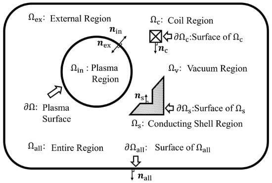
Figure 2.
The integral regions. , , , and are the plasma, conducting shells, coils, and vacuum regions, respectively. The plasma surface is assumed to coincide with the magnetic surface. and are the surfaces of coils and conducting shells, respectively. is the external region. stands for the entire region consisting of plasma and external regions, and is the outside surface of . The , , , , and are the outward unit normal vector of the plasma, external, coil, conducting shell, and entire regions, respectively.
Taking the variations of Equation (12) under the constraints of adiabatic condition and magnetic flux conservation of plasma, magnetic flux conservation of conducting shells, and the current conservation of coils, the following two equations are obtained as the Euler–Lagrange equations, which are derived in Appendix A,
where is the jump of f at the boundary of the two regions and is given by
where the subscripts “ex” and “in” mean the outside and the inside of the boundary, respectively. Equation (13) is the MHD equilibrium equation and Equation (14) shows the pressure balance at the plasma surface. Therefore, the state that minimizes the energy functional (12) is the equilibrium state of the ideal MHD equation. Since the energy function (11) is a discrete approximation of the functional (12), the numerical solution of the MLM that minimizes the free energy (11) coincides with the equilibrium solution of the ideal MHD equation.
Next consider the energy conservation. The total system energy of the MLM model including current sources is conserved, as shown in Appendix B,
where and are mass density and plasma velocity, respectively. Therefore, the total system energy of plasma kinetic energy and the free energy , which includes work by current sources, is conserved, as is expected from Equation (4). Since the sum of free energy and kinetic energy is conserved, the application to MHD stability analysis is expected by the use of free energy instead of potential energy. The third term on the right-hand side of Equation (12) apparently resembles the vacuum magnetic energy term in the VMEC free boundary problem [], where its variation keeps the plasma current constant, while variation of changes plasma current under the constraint of constant magnetic flux.
Since the magnetic flux and current in the circuit system are related by inductance matrix ,
and of the right-hand side in Equation (11) are evaluated by Equation (17). Equation (17) can be rewritten as
where the subscript specifies the flux conservation system () or the current constant system (). , , , and in Equation (11) are elements of , , , and , respectively. Although plasma displacement changes the values of , , and , the valudes of and are determined from the given values of and using the simultaneous linear Equation (18).
In the 3-D MLM, the mutual inductance of the ith and jth coils is given by the Neumann formula,
where and are the position vector and its trajectory of the ith filament shown in Figure 1c, respectively. Since Equation (19) cannot be used to calculate self-inductance, the self-inductance of a circular filament is employed as an approximation. For a circular filament, D is the radius of the circular loop, while d denotes the radius of the filament’s cross section. When the condition is satisfied, the self-inductance L can be approximated by the following expression [],
where is internal inductance, which is determined by the current distribution within the cross section of the conductor. In this study, is chosen, which means the uniform current density. Then the self-inductance is obtained from Equation (20),
where and are the length and radius of the ith filamentary circuit, respectively. Here D in Equation (20) is replaced by the length of filaments . In this study, Equation (21) is used for imaginary filaments of plasma shown in Figure 1c because those filaments are sufficiently thin and similar to circular circuits. For simplicity, the magnetic field coils also employ Equation (21) since their values do not affect the plasma equilibrium. As was explained in this section, the filaments are introduced to simulate the current distribution on the current layers. Therefore, the filament radius is determined so that their combined inductance coincides with the self-inductance of the current layer.
As the matrix is determined by the configuration of the coil and plasma, the free energy is also a function of the configurations of the plasma, which are represented by in Equation (10). Here, the shape of each current layer k (Figure 1a) is represented by the next Fourier series.
where and denote the cylindrical coordinates in Equations (1)–() of the kth current layer, and , , , and are their cosine and sine Fourier coefficients. Here, m and n denote the poloidal and toroidal mode numbers, respectively, and is the toroidal angle. The geometrical axis of kth current layer is determined by Equations (22) and (23) with . Using the axis, the poloidal angle on the kth layer is determined as the angle around the axis. Although our model does not prescribe a current layer to the magnetic axis, the axis of the innermost current layer corresponds to the magnetic axis. Since, in this work, is chosen as the set of Fourier coefficients , , , and in Equations (22) and (23), the inductance matrix is a function of variable .
Finally, the computational procedure of the 3-D MLM is summarized as follows. The continuous model requires the coil orbits and currents, poloidal flux distribution as a function of toroidal flux , entropy parameter distribution , and initial geometrical configuration of plasma. In the descret model of the 3-D MLM, the coil orbits and currents, toroidal and poloidal fluxes and of each plasma current layer, entropy parameters , and the initial plasma shape are required for the minimization of the free energy (11). The coil currents, , , and , are fixed during the minimization process, whereas the plasma configuration parameters are updated at every iteration. The 3-D MLM assumes the existence of nested closed magnetic surfaces in the plasma region, as VMEC. The toroidal and poloidal plasma current distributions on the current layers are then determined under the assumption that the current layers coincide with magnetic surfaces. These distributed currents are represented by toroidal and poloidal filamentary circuit currents. The inductance matrix is evaluated by Equations (19) and (21), based on the plasma filaments and the coils orbits. In the axisymmetric MLM, mutual inductances in the toroidal direction can be calculated using incomplete elliptic integrals, whereas they are evaluated by Equations (19) and (21) in the 3-D MLM. Moreover, the poloidal current can be represented as a surface current in the axisymmetric version, and mutual inductances between toroidal and poloidal systems are exactly zero. Since these relations are not used in non-axisymmetric configurations, the plasma current distribution and the flux linkage of the coils are then obtained by Equation (18). In addition, the volume between plasma current layers is a function of , and the pressure distribution is determined by Equation (8). These procedures are repeated to search for the plasma configuration that minimizes the free energy, which represents the equilibrium solution. In this study, the simplex method [] is used in the minimization.
3. Numerical Examples
In this section, two numerical examples have been demonstrated to confirm the validity of the 3-D MLM. In Section 3.1, a vacuum magnetic field of a stellarator is used to compare the equilibrium solution of the MLM. In Reference [], our research group has investigated the non-axisymmetric effects of saddle coils (SCs) of the small tokamak PHiX. In Section 3.2, the data of PHiX are used to calculate the non-axisymmetric equilibrium solutions, whose MLM and VMEC solutions are compared. As shown in Table 1, the MLM requires the flux and entropy distributions. Hence, these distributions must be extracted from the reference equilibria to be compared.

Table 1.
Required parameters of 3-D MLM and corresponding input parameters of VMEC.
3.1. Comparison with Stellarator’s Vacuum Magnetic Surfaces
In this subsection, the non-axisymmetric equilibrium solution of the 3-D MLM is compared with the vacuum magnetic surfaces of a stellarator to check the accuracy of the 3-D MLM. In the cylindrical coordinate system , consider a helical coil whose orbit is
where is the poloidal angle around the geometrical axis . The magnetic surfaces exist when the magnetic field has a symmetry. To realize approximate helical symmetry in a toroidal system, a sufficiently large aspect ratio of the helical coil is required. In this work, , m, m, and are choosen. The blue and black symbols in Figure 3 indicate the positions and current directions of two pairs of helical coils. The first pair of the helical coils with has a positive current of 15 A·turn for each coil, while the other pair of the helical coils with has a negative current of A·turn for each coil. As shown in Figure 3a, two pairs of helical coils with blue and black symbols return to the same positions on the poloidal cross section with intervals of . In this stellarator, the magnetic surface cross sections are elliptical [], and the stellarator has a toroidal periodicity of . The toroidal magnetic field is generated by sixteen rectangular TFCs, with current of 80 kA·turn, placed at intervals of , starting from . The four vertices of each TFC are , , , and m, respectively. To represent the magnetic surface shape of this stellarator, the Fourier modes and in Equations (22) and (23) are required. In this work, the mode ranges are set to and . Since the TFCs are positioned far from the helical coils, the mode is neglected. The number of Fourier coefficients in Equations (22) and (23) of each current layer is 190.

Figure 3.
Poincaré plots of the vacuum magnetic field at torodal angles , , , . The blue and black symbols indicate the locations and current direction of the helical coils. The black lines indicate the current layers determined by 3-D MLM calculation. (a) Poincaré plots of the vacuum magnetic field created by TF and helical coils. (b) Poincaré plots of the magnetic field by the 3-D MLM calculation result.
The magnetic field lines of this stellarator are calculated using field line tracing. Figure 3a shows Poincaré plots of this stellarator’s vacuum magnetic field, demonstrating the existence of closed magnetic surfaces with elliptical cross sections in the central region. In the region outside these closed surfaces, stochastic regions appear where no magnetic surfaces exist. Then, the magnetic fluxes of some closed magnetic surfaces are calculated and used as input parameters for the 3-D MLM. Toroidal flux and poloidal flux on a magnetic surface are calculated from line integrals over the surface obtained by the Poincaré plots:
where and are poloidal and toroidal paths that lie on the surface and encircle the magnetic axis and the Z axis, respectively. These paths are similar to the imaginary filaments shown in Figure 1c. Using Equations (27) and (28), the distributions of normalized poloidal flux are obtained as functions of the normalized toroidal flux shown in Figure 4, where both of the normalized fluxes are defined to be unity at the plasma surface while they are zero at the magnetic axis. The blue dots in Figure 4 show the normalized poloidal fluxes of which the data circled in red are used in the MLM calculation for current layers. Therefore, the allocated flux distributions of the MLM are the same as those of the vacuum field. The initial Fourier coefficients in Equations (22) and (23) of 4 current layers are chosen from those closed magnetic surfaces shown in Figure 3a and are used in the 3-D MLM. The total number of Fourier coefficients is . As was explained in the previous section, the current distribution on a current layer is represented by those of imaginary filaments. In this example, every current layer is represented by 40 toroidal imaginary filaments and 120 poloidal filaments. The inductance matrix in Equation (17) is calculated by Equations (19) and (21) from the 660 orbits of plasma imaginary filaments and coils. It is a symmetric square matrix with the size of elements, of which only about half need to be computed. The parameters required for calculating the self-inductance (21) of plasma imaginary filaments are summarized in Table 2, in which the values on the outermost current layer are listed as the representative value. Here, is specified and fixed during the minimization process, while is determined from the filament orbit. The aspect ratios are sufficiently large, and Equation (21) is therefore applicable.
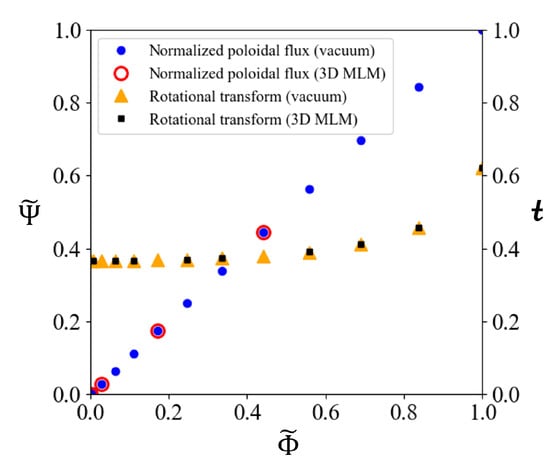
Figure 4.
Distributions of the normalized poloidal flux (left axis) and the rotational transform (right axis) against the normalized toroidal flux of the stellarator’s vacuum magnetic field. The blue dots are the normalized poloidal fluxes, of which those circled in red are used in the MLM calculation. The orange triangles are the rotational transforms of the vacuum magnetic field, and the black squares are those of the 3-D MLM solution.
Table 2.
Parameters of plasma imaginary filament on the outermost current layers in the stellarator configuration.
First, the shapes of the current layers and the traced magnetic surfaces in the 3-D MLM solution are compared with the closed magnetic surfaces of the stellarator’s vacuum magnetic field. Figure 3b presents the Poincaré plots of the 3-D MLM solution. Because only closed magnetic surfaces are compared, stochastic regions are excluded from Figure 3b. The black lines in Figure 3a,b indicate the current layers obtained by the 3-D MLM in which the current layers coincide with magnetic surfaces. Figure 3a shows that these current layers nearly coincide with the vacuum magnetic surfaces in red. The closed magnetic surfaces in Figure 3b, where the orange dots are Poincaré plots of magnetic fields that are evaluated by the current of coils and current layers, show good agreement with the corresponding surfaces (red) in Figure 3a for the stellarator’s vacuum magnetic field.
Since it is a vacuum magnetic field, the electric currents at the current layer must be zero. According to the MLM result, the total current of the poloidal filament is five orders of magnitude smaller than that of the TFCs, and the toroidal filament total current is also five orders of magnitude smaller than the current in the helical coils. Consequently, the magnetic field of the MLM result is identical to that of the stellarator’s vacuum magnetic field, since the surface currents of the MLM result can be negligible. As a result, the magnetic field is created only by the external coil currents. Therefore, the rotational transform obtained from the MLM solution also coincides with that of the vacuum field, as shown in Figure 4, in which the rotational transform of the magnetic surface is given by
where is the rotational transform angle and is the number of rotations around the Z axis. The black squares in Figure 4 are the rotational transforms of the 3-D MLM solution, while the orange triangles are those of the vacuum magnetic field. The two results show good agreement in the plasma region.
In summary, this subsection presents a validation of the 3-D MLM through comparison with the vacuum magnetic field of a stellarator. The current layers obtained from the MLM are nearly identical to the magnetic surfaces of the vacuum field. The surface currents on the current layers are several orders of magnitude smaller than the coil currents and are negligible. These results demonstrate that the 3-D MLM can obtain the equilibrium equivalent to the stellarator vacuum magnetic fields.
3.2. Comparison with VMEC Equilibrium
In this subsection, the non-axisymmetric equilibrium solution of the 3-D MLM is compared with the non-axisymmetric equilibrium solution of VMEC to check the accuracy of the 3-D MLM. The parameters of the device model are set to a major radius of m, a minor radius of m, and a plasma current of kA, following the values of the small tokamak PHiX []. Equations (1)–(3) are used to convert from the cylindrical coordinate system to the Cartesian coordinate system . The locations and current directions of the SCs are shown in Figure 5a. The SC current of each coil is 3.6 kA·turn. Sixteen rectangular TFCs, each with a current of 9.36 kA·turn, are placed at intervals of , starting from . The location of a TFC in the poloidal cross section is shown in Figure 5b. Only two PFCs, located at m, as shown in Figure 5b, are used in the calculations, in which the current of each PFC is kA·turn. The same geometry and currents of the magnetic coils are used in the calculations of the 3-D MLM and VMEC. In this study, the directions of the current of TFCs and SCs are the same as in Reference [], whose Figure 2b is the Poincaré plots of a vacuum magnetic field at , where the magnetic surfaces are almost symmetric about the R axis. Then, only the cosine term in Equation (22) and the sine term in Equation (23) are used in 3-D MLM and VMEC,
As shown in Figure 5a, the SCs are arranged. Accordingly, the Fourier modes used in Equations (30) and (31) are set to and . The total number of Fourier coefficients in Equations (30) and (31) is for current layers in the 3-D MLM calculation and 9100 for 100 magnetic surfaces in the VMEC calculation. As summarized in Table 1, both methods require initial Fourier coefficients. In the 3-D MLM, these coefficients are specified for all current layers, whereas VMEC requires only the coefficients of the outermost magnetic surface and the magnetic axis. In this work, the initial Fourier coefficients of the outermost current layer in the MLM are selected to be the same as those of the outermost magnetic surface in the VMEC calculation.

Figure 5.
(a) Locations of saddle coils (SCs) on the small tokamak PHiX. The red lines are the SCs, whose black arrows indicate the direction of the current. (b) Example of an axisymmetric equilibrium configuration of PHiX. The closed black circle is a current layer of the plasma. The red dots are the locations of poloidal field coils (PFCs), and the gray line is the toroidal field coil (TFC).
In the 3-D MLM calculation, each current layer consists of 40 toroidal and 120 poloidal imaginary filaments, whose parameters on the outermost current layers are listed in Table 3 as the representative values, in which the aspect ratios of filaments are sufficiently large for Equation (21). Including both plasma filaments and coils, the total number of circuits is 1628. The inductance matrix in Equation (17) is a square matrix of dimension , containing 2,650,384 elements.
Table 3.
Parameters of plasma imaginary filament on the outermost current layers in the PHiX configuration.
The input parameters of VMEC and the 3-D MLM are listed in Table 1. In this study, and p profiles in VMEC are prescribed as the functions of the normalized toroidal flux, although VMEC can choose the current profile instead of the profile. The red line in Figure 6 indicates the distribution of the VMEC profile. Plasma poloidal flux at toroidal flux can be calculated by
where function is the rotational transform. The blue line in Figure 6 shows the normalized poloidal flux distribution, obtained from Equation (32) using the profile of VMEC. Using this VMEC profile, poloidal and toroidal fluxes of the current layers of the MLM are selected, which are depicted by black squares in Figure 6. The pressure distribution used in VMEC is
where is the pressure at the magnetic axis, whose value is selected so that the total value is about . The normalized pressure is shown by the black line in Figure 7. The corresponding entropy parameters in Equation (8) are allocated by Equation (33). Using these distributions, a 3-D MLM solution is obtained.

Figure 6.
Distributions of the normalized poloidal flux (left axis) and the rotational transform (right axis) against the normalized toroidal flux . The black squares show the poloidal and toroidal fluxes used in the MLM calculation at the given current layers. The blue line shows the normalized poloidal flux distribution, which is obtained from Equation (32). The gray dots are the rotational transforms evaluated by tracing the magnetic field lines in the MLM equilibrium result. The red line is the rotational transform used in the VMEC calculation.
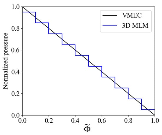
Figure 7.
Distributions of normalized pressure against normalized toroidal flux . The black and blue lines represent the pressure distributions of the VMEC input profile and the MLM solution, respectively. Both distributions are normalized by the maximum pressure in Equation (33).
The rotational transform distributions obtained from the two methods are compared. The gray dots in Figure 6 represent the rotational transform calculated by field line tracing in the MLM solution. Although the rotational transforms are discontinuous at the current layers, these values follow the red line of the prescribed values in VMEC, confirming that the rotational transform profiles of the two solutions are almost identical. Figure 7 compares the pressure profiles. Although the MLM model assumes uniform pressure between current layers, the pressure distribution of the 3-D MLM resembles that of VMEC.
Next, a comparison of the plasma cross sections is shown in Figure 8. The poloidal cross sections of the 3-D MLM and VMEC equilibria are reconstructed from the obtained Fourier series in Equations (30) and (31). The magnetic surfaces of the VMEC solution at four different toroidal angles are illustrated in Figure 8a, while Figure 8b shows the cross sections of the current layers, which also correspond to magnetic surfaces, for the 3-D MLM solution. These figure shows that the current layers of the MLM solution (b) are almost identical to the magnetic surfaces of the VMEC solution (a). This agreement is further quantified through a comparison of the Fourier coefficients between the 3-D MLM and VMEC solutions. Since the current layers in the MLM model exactly coincide with magnetic surfaces, the same Fourier series in Equations (30) and (31) are chosen. Figure 9 shows five dominant Fourier coefficients of the outermost magnetic surface in VMEC, and those of the outermost current layer in the 10-layer MLM model, where the toroidal flux of the outermost current layer in the MLM model is chosen to have the same value of the outermost magnetic surface in the VMEC solution. According to the figure, the Fourier coefficients of the MLM solution are almost the same as those of the VMEC solution, indicating that the cross sections obtained from 10-layer MLM models are in good agreement with those from the VMEC calculation using 100 magnetic surfaces, as shown in Figure 8. Finally, the plasma currents obtained from the 3-D MLM and VMEC solutions are compared. The MLM solution gives A, while the VMEC solution yields A, whose relative difference is
which means that the plasma current in the MLM solution is in good agreement with that of the VMEC solution.
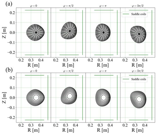
Figure 8.
A comparison of equilibrium configurations at toroidal angles , , , for the same coil currents and rational transform distributions. (a) Poloidal cross sections of magnetic surfaces of the VMEC equilibrium solution. (b) Poloidal cross sections of current layers of the 10-layer MLM equilibrium solution. The green lines represent the layers on which the SCs shown in Figure 5 are wound.

Figure 9.
A comparison between equilibrium Fourier coefficients of the outermost magnetic surface of VMEC and those of the outermost current layer of the 10-layer MLM model. The vertical axis is the value of the Fourier coefficients. and are Fourier coefficients, defined in Equations (30) and (31). The integers in parentheses are the poloidal and toroidal mode numbers.
In summary, the comparative study in this subsection demonstrates that the 3-D MLM and VMEC obtain an almost identical equilibrium solution.
These results validate the 3-D MLM for calculating non-axisymmetric plasma equilibria. As is shown in this section, the non-linear free energy function (11) with many (910) arguments consists of a large size () inductance matrix whose calculation requires a lot of numerical integrations. Although the calculations can be accelerated through parallelization, it has not yet been implemented. Therefore, the computational performance of the 3-D MLM is approximately 30 times slower than that of VMEC. Then the parallelization remains a future task.
4. Conclusions
The 3-D MLM has been developed to obtain the 3-D free boundary MHD equilibrium. Based on the variational principle, MHD equilibrium is obtained as the minimum energy state of the free energy functional whose Euler–Lagrange equation is identical with the MHD equilibrium equation. The tokamak device is modeled as a system consisting of a plasma, conducting shells, and coils with current sources. Since the discretized free energy equation, Equation (11), is an approximation of Equation (12), the equilibrium solution of the MLM that minimizes the free energy (11) coincides with the equilibrium solution of the ideal MHD equation.
In order to confirm the validity of our method, a vacuum magnetic field of a stellarator was compared with a magnetic field obtained by the 3-D MLM. The magnetic field obtained as an equilibrium solution by the 3-D MLM is almost identical to the stellarator vacuum field. Next, using the design values of PHiX, a non-axisymmetric equilibrium solution of the 3-D MLM was compared with a solution of VMEC. The equilibrium solution obtained by the MLM is nearly identical to the equilibrium solution of VMEC. Therefore, the validity of the 3-D equilibrium calculation by the MLM was confirmed based on the above results.
The conventional axisymmetric tokamak control simulation codes are unable to include non-axisymmetric effects, while 3-D equilibrium solvers originally developed for stellarators do not include conducting structures. The 3-D equilibrium solvers using magnetic coordinates cannot include a separatrix that is essential in tokamak control studies. To solve these limitations, the 3-D MLM is developed.
In future work, the 3-D MLM will be extended and improved in several directions. First, although many developed codes use electric current and pressure distributions rather than magnetic fluxes and entropy parameters as input parameters, the current version of the 3-D MLM requires the toroidal and poloidal fluxes and entropy distribution. To improve usability, the model will be modified to accept current and pressure distributions as input. Second, the 3-D MLM will be adapted for high-speed parallel computation to improve performance for equilibrium calculations. Third, future research will focus on extending the 3-D MLM to dynamic simulations, allowing for the incorporation of feedback control systems. Such developments will establish the method as a comprehensive tool for control studies in tokamak plasma with the effect of non-axisymmetric magnetic fields and a separatrix.
Author Contributions
Conceptualization, H.T.; methodology, J.W. and H.T.; software, J.W.; validation, J.W.; formal analysis, J.W.; investigation, J.W.; resources, J.W.; data curation, J.W.; writing—original draft preparation, J.W.; writing—review and editing, H.T.; visualization, J.W.; supervision, H.T.; project administration, H.T.; funding acquisition, H.T. All authors have read and agreed to the published version of the manuscript.
Funding
This research was funded by Japan Society for the Promotion of Science KAKENHI Grant Number 21H01061.
Institutional Review Board Statement
Not applicable.
Informed Consent Statement
Not applicable.
Data Availability Statement
The data presented in this study are available upon request from the corresponding author.
Conflicts of Interest
The authors declare no conflicts of interest.
Abbreviations
The following abbreviations are used in this manuscript:
| MHD | magnetohydrodynamics |
| 3-D | three-dimensional |
| MLM | Multi-Layers Method |
| TFC | toroidal field coil |
| PFC | poloidal field coil |
| SC | saddle coil |
Appendix A. Euler–Lagrange Equation with Coils
As shown in Figure 2, the entire space () is divided into two regions, the plasma region () and the external region () that consists of three sub-regions of the coils (), the conducting shells (), and the vacuum region (). The boundary between the plasma region and the external region is the surface of the plasma (), and is assumed to coincide with the magnetic surface. The integral over the vacuum region is identically zero in the MLM model, since is assumed to vanish in the vacuum region where no current flows. In order to extend the domain of integration to the entire region, this integral term is added to the free energy (12). As shown in Equation (A1), the free energy consists of the following five terms,
Equation (A1) can be reduced to
Since , the following equation can be obtained from Equation (A2),
Using Gauss’ theorem and vector formula , Equation (A3) can be reduced to
where is the outside surface of , as shown in Figure 2. Although Gauss’ theorem is applied to multiply connected region (torus), the surface integrals at the cut surfaces (poloidal cross section) to make the torus into a single-connected region cancel each other, and since the magnetic field decays fast enough far away from the plasma and coils, the surface integral at converges to zero as the domain is made infinitely large. Then, Equation (A4) can be reduced to
When the plasma is deformed by displacement , the deformation of its surface (boundary with the external region) must also be taken into account (Figure A1). Taking a variation of a functional of f, the next relation is satisfied,
Using the displacement of the ideal and adiabatic plasma, the perturbations of and p are
respectively []. Since and for , the following relation can be obtained from Equation (A8),
in the plasma region. At the plasma–vacuum interface, using vector formula ,
is satisfied since the electric field parallel to the boundary is continuous and
is assumed on the plasma surface.

Figure A1.
Perturbed boundary when the plasma is deformed by displacement . The hatched area represents a small area element on the boundary surface. Here is the outward unit normal vector of the surface.
First, take the variation of the magnetic energy of the plasma region in Equation (A6) using Equation (A7),
Substituting Equations (A10) and (A11) for Equation (A13),
is obtained.
Next, take the variation of the external region similar to the plasma region. Here, in because the coil current is assumed to be constant while in because the conducting shell’s magnetic flux is assumed to be conserved. Because of at the vacuum side of the plasma–vacuum interface , using Equation (A7), the variation of the magnetic energy of the external region in Equation (A6) is
Since in and no current flows in the vacuum region , the integral term in the domains and is zero. Then, using Gauss’ theorem, Equation (A15) can be reduced to
Since decays fast enough far away from the plasma, coils, and conducting shells, the surface integral at converges to zero as the domain is made infinitely large. Then, Equation (A16) can be reduced to
Substituting Equation (A11) for Equation (A17),
is obtained.
Taking the variations of internal energy in Equation (A6) under the constraint of Equation (A9) using Equation (A7),
can be obtained. Using , Equation (A19) can be reduced to
Then, using Gauss’ theorem,
is obtained from Equation (A20).
In describing the boundary conditions, the change of the physical variables f at the boundary is introduced,
where the subscript specifies the outside of the boundary () or the inside of the boundary (). Therefore, taking the variations of Equation (12) under the constraints of an adiabatic condition and magnetic flux conservation of plasma and the current conservation of coils,
is obtained from Equations (A14), (A18), and (A21) because of on . Therefore, the following Euler–Lagrange equations of Equation (12) are obtained,
where Equation (A24) is the MHD equilibrium equation and Equation (A25) is the equation for pressure balance on the plasma surface. When the plasma surface is fixed, the results are consistent with those of well-known Reference [].
Appendix B. Energy Conservation of Plasma–Coil System
The energy conservation equation in the ideal MHD without dissipation is as follows []:
where is an electric field. The first term on the left side of Equation (A26) represents the rate of change of plasma energy density consisting of the kinetic, magnetic, and internal energies. The second term on the left side of Equation (A26) corresponds to the kinetic and internal energy fluxes, the mechanical work by pressure, and the flux of electromagnetic energy represented by the Poynting vector .
The sum of free energy () and kinetic energy is given by
where , , and W are defined by
In the case of free boundary problems, the movement of the plasma surface (boundary with the external region) must also be taken into account, similarly to the displacement of plasma shown in Figure A1. Similar to Equation (A7), the time derivative of the volume integral of a function f is given by
Therefore, similar to Equation (A11),
is satisfied on the plasma–vacuum interface .
Using Equations (A26) and (A31), the rate of change of (A28) is
Then, using Gauss’ theorem, Equation (A33) can be reduced to
Substituting Equation (A32) for Equation (A34),
is obtained.
Using Equation (A31) and Faraday’s law , the rate of change of (A29) is
Using Gauss’ theorem and vector formula , Equation (A36) can be reduced to
where is the outside surface, as shown in Figure 2. Since decays fast enough far away from the plasma, coils, and conducting shells, the surface integral at converges to zero as the domain is made infinitely large. Then, Equation (A37) can be reduced to
Substituting Equation (A32) for Equation (A38),
because of on .
Since is constant in time in , the rate of change W (A30) is
The right-hand side of Equation (A40) corresponds to the last term on the right-hand side of Equation (4), which is the work by current sources. Since in and no current flows in the vacuum region , the integral term in the domains and is zero.
Then, using Equations (A35), (A39), and (A40), the rate of change of Equation (A27) is
The rate of change of corresponds to the first term on the right-hand side of Equation (4). The rate of change of W corresponds to the last term on the right-hand side of Equation (4), which is the work by current sources. Therefore, the total system energy, consisting of plasma kinetic energy and the free energy , which includes work by current sources, is conserved.
References
- Okabayashi, M.; Bialek, J.; Chance, M.S.; Chu, M.S.; Fredrickson, E.D.; Garofalo, A.M.; Gryaznevich, M.; Hatcher, R.E.; Jensen, T.H.; Johnson, L.C.; et al. Active feedback stabilization of the resistive wall mode on the DIII-D device. Phys. Plasmas 2001, 8, 2071–2082. [Google Scholar] [CrossRef]
- Strait, E.J.; Bialek, J.M.; Bogatu, I.N.; Chance, M.S.; Chu, M.S.; Edgell, D.H.; Garofalo, A.M.; Jackson, G.L.; Jayakumar, R.J.; Jensen, T.H.; et al. Resistive wall mode stabilization with internal feedback coils in DIII-D. Phys. Plasmas 2004, 11, 2505–2513. [Google Scholar] [CrossRef]
- Evans, T.; Moyer, R.; Burrell, K.; Fenstermacher, M.E.; Joseph, I.; Leonard, A.W.; Osborne, T.H.; Porter, G.D.; Schaffer, M.J.; Snyder, P.B.; et al. Edge stability and transport control with resonant magnetic perturbations in collisionless tokamak plasmas. Nat. Phys. 2006, 2, 419–423. [Google Scholar] [CrossRef]
- Liang, Y.; Bialek, J.M.; Bogatu, I.N.; Chance, M.S.; Chu, M.S.; Edgell, D.H.; Garofalo, A.M.; Jackson, G.L.; Jayakumar, R.J.; Jensen, T.H.; et al. Active control of type-I edge localized modes on JET. Plasma Phys. Control. Fusion 2007, 49, 2505–2513. [Google Scholar] [CrossRef]
- Neumeyer, C.; Koslowski, H.R.; Thomas, P.R.; Nardon, E.; Jachmich, S.; Alper, B.; Andrew, P.; Andrew, Y.; Arnoux, G.; Baranov, Y.; et al. Design of the ITER In-Vessel Coils. Fusion Sci. Technol. 2011, 60, 95–99. [Google Scholar] [CrossRef]
- Daly, E.F.; Ioki, K.; Loarte, A.; Martin, A.; Brooks, A.; Heitzenroeder, P.J.; Kalish, M.; Neumeyer, C.; Titus, P.; Zhai, Y.; et al. Update on Design of the ITER In-Vessel Coils. Fusion Sci. Technol. 2013, 64, 168–175. [Google Scholar] [CrossRef]
- Matsunaga, G.; Takechi, M.; Sakurai, S.; Suzuki, Y.; Ide, S.; Urano, H. In-vessel coils for magnetic error field correction in JT-60SA. Fusion Eng. Des. 2015, 98–99, 1113–1117. [Google Scholar] [CrossRef]
- Murakami, H.; Matsunaga, G.; Takechi, M.; Sukegawa, A.; Sakurai, S.; Kizu, K.; Tsuchiya, K.; Koide, Y.; Yoshida, K. Thermal and Mechanical Design of Error Field Correction Coil for JT-60SA. IEEE Trans. Appl. Supercond. 2016, 26, 4204805. [Google Scholar] [CrossRef]
- Mastrostefano, S.; Bettini, P.; Bolzonella, T.; Furno Palumbo, M.; Liu, Y.Q.; Matsunaga, G.; Specogna, R.; Takechi, M.; Villone, F. Three-dimensional analysis of JT-60SA conducting structures in view of RWM control. Fusion Eng. Des. 2015, 96–97, 659–663. [Google Scholar] [CrossRef]
- ArchMiller, M.C.; Cianciosa, M.R.; Ennis, D.A.; Hanson, J.D.; Hartwell, G.J.; Hebert, J.D.; Herfindal, J.L.; Knowlton, S.F.; Ma, X.; Maurer, D.A.; et al. Suppression of vertical instability in elongated current-carrying plasmas by applying stellarator rotational transforma. Phys. Plasmas 2014, 21, 056113. [Google Scholar] [CrossRef]
- Sakurai, K.; Tanahashi, S. Positional Stability of a Current-Carrying Plasma in an l=2 Stellarator Field. J. Phys. Soc. Jpn. 1980, 49, 759–762. [Google Scholar] [CrossRef]
- Naito, S.; Murayama, M.; Hatakeyama, S.; Kuwahara, D.; Suzuki, Y.; Tsutsui, H.; Tsuji-Iio, S. Stabilization of vertical plasma position in the PHiX tokamak with saddle coils. Nucl. Fusion 2021, 61, 116035. [Google Scholar] [CrossRef]
- Yasuda, K.; Fujita, T.; Okamoto, A.; Arimoto, H.; Kimata, S.; Kado, K.; Tsunoda, K. Stabilization of plasma vertical position of elongated tokamak using upper and lower triangular coils. Phys. Plasmas 2021, 28, 082108. [Google Scholar] [CrossRef]
- Yushmanov, P.N.; Takizuka, T.; Riedel, K.S.; Kardaun, O.J.W.F.; Cordey, J.G.; Kaye, S.M.; Post, D.E. Scalings for tokamak energy confinement. Nucl. Fusion 1990, 30, 1999–2006. [Google Scholar] [CrossRef]
- Jardin, S.C.; Pomphrey, N.; Delucia, J. Dynamic modeling of transport and positional control of tokamaks. J. Comput. Phys. 1986, 66, 481–507. [Google Scholar] [CrossRef]
- Khayrutdinov, R.R.; Lukash, V.E. Studies of Plasma Equilibrium and Transport in a Tokamak Fusion Device with the Inverse-Variable Technique. J. Comput. Phys. 1993, 109, 193–201. [Google Scholar] [CrossRef]
- Hirshman, S.P.; Whitson, J.C. Steepest-descent moment method for three-dimensional magnetohydrodynamic equilibria. Phys. Fluids 1983, 26, 3553–3568. [Google Scholar] [CrossRef]
- Harafuji, K.; Hayashi, T.; Sato, T. Computational study of three-dimensional magnetohydrodynamic equilibria in toroidal helical systems. J. Comput. Phys. 1989, 81, 169–192. [Google Scholar] [CrossRef]
- Tsutsui, H.; Shimada, R. Equilibrium Analysis of Tokamak Plasma by Multi-Layers Method. J. Plasma Fusion Res. 1996, 72, 1252–1258. [Google Scholar]
- Tsutsui, H.; Shimada, R. Dynamic Analysis of Tokamak Plasma by Multi-layers Method. J. Plasma Fusion Res. 1999, 75, 176–185. [Google Scholar] [CrossRef]
- Jardin, S.C.; Larrabee, D.A. Feedback stabilization of rigid axisymmetric modes in tokamaks. Nucl. Fusion 1982, 22, 1095–1098. [Google Scholar] [CrossRef]
- Panofsky, W.K.H.; Phillips, M. Classical Electricity and Magnetism, 2nd ed.; Dover Publications: New York, NY, USA, 2005; p. 174. ISBN 978-0486439242. [Google Scholar]
- Miyamoto, K. Equilibrium. In Fundamentals of Plasma Physics and Controlled Fusion, 1st ed.; Iwanami Book Service Center: Tokyo, Japan, 1997; p. 83. ISBN 4-900491-11-X. [Google Scholar]
- Nelder, J.A.; Mead, R. A Simplex Method for Function Minimization. Comp. J. 1965, 7, 308–313. [Google Scholar] [CrossRef]
- Miyamoto, K. Non-Tokamak Confinement System. In Fundamentals of Plasma Physics and Controlled Fusion, 1st ed.; Iwanami Book Service Center: Tokyo, Japan, 1997; pp. 325–327. ISBN 4-900491-11-X. [Google Scholar]
- Miyamoto, K. Magnetohydrodynamic Instabilities. In Fundamentals of Plasma Physics and Controlled Fusion, 1st ed.; Iwanami Book Service Center: Tokyo, Japan, 1997; p. 128. ISBN 4-900491-11-X. [Google Scholar]
- Kruskal, M.D.; Kulsrud, R.M. Equilibrium of a Magnetically Confined Plasma in a Toroid. Phys. Fluids 1958, 1, 265–274. [Google Scholar] [CrossRef]
- Freidberg, J.P. Ideal MHD, 1st ed.; Cambridge University Press: Cambridge, UK, 2014; p. 47. ISBN 978-1-107-00625-6. [Google Scholar]
Disclaimer/Publisher’s Note: The statements, opinions and data contained in all publications are solely those of the individual author(s) and contributor(s) and not of MDPI and/or the editor(s). MDPI and/or the editor(s) disclaim responsibility for any injury to people or property resulting from any ideas, methods, instructions or products referred to in the content. |
© 2025 by the authors. Licensee MDPI, Basel, Switzerland. This article is an open access article distributed under the terms and conditions of the Creative Commons Attribution (CC BY) license (https://creativecommons.org/licenses/by/4.0/).