Efficient Three-Dimensional Marine Controlled-Source Electromagnetic Modeling Using Coordinate Transformations and Adaptive High-Order Finite Elements

Abstract

Efficient and accurate forward modeling of electromagnetic fields is essential for advancing geophysical exploration in complex marine environments. However, realistic survey conditions characterized by low-frequency spectra, fine sedimentary strata, irregular bathymetry, and anisotropic materials pose significant challenges for conventional numerical methods. To address these issues, this work presents a parallel modeling framework that combines coordinate transformations with an adaptive high-order finite-element approach for 3D marine controlled-source electromagnetic (MCSEM) simulations. The algorithm exploits the form invariance of Maxwell’s equations to map the original boundary value problem over the physical domain to one defined over a computationally favorable domain filled with anisotropic media. The transformed model is then discretized and solved using a parallel high-order finite-element scheme enhanced with a goal-oriented adaptive mesh refinement strategy. We examine the performance of the proposed framework using both synthetic models and the realistic Marlim R3D benchmark dataset. The results demonstrate that the proposed approach can effectively reduce computational costs while maintaining high accuracy across a wide frequency range and varying water depths. These findings highlight the framework’s potential for large-scale, high-resolution CSEM exploration of offshore resources.

1. Introduction

Marine controlled-source electromagnetic (MCSEM) methods have gained wide recognition as a powerful tool for imaging offshore geological structures and identifying submarine resources [1]. These applications rely on towed electric sources and arrays of seafloor or streamer-based receivers to infer the electrical conductivity distribution of the subsurface [2]. Modern acquisition systems are able to conduct large-scale 3D MCSEM surveys [3]. The rich data coverage processed at a few discrete low frequencies helps improve the model resolution at different scales. During the interpretation process, electrical anisotropy is often considered according to the support from well log data. A common case is the vertical transverse isotropy (VTI) due to sedimentary layering [4,5]. However, geological activities such as folding and faulting often disrupt the idealized layered models, resulting in complex anisotropy patterns [6]. Recent studies have demonstrated the significant impact of complex electrical anisotropy, such as the tilted transverse isotropy (TTI), on MCSEM responses [7,8,9], highlighting the need for more advanced and reliable interpretation tools.

Accurate and efficient forward modeling is fundamental to the success of MCSEM data interpretation, particularly in environments characterized by strong anisotropy and geometrical complexity. To this end, a variety of numerical approaches have been proposed, including finite-difference [10], integral-equation [11], finite-volume [12], and finite-element methods [13,14,15,16]. Among these, finite-element techniques are especially attractive due to their flexibility in accommodating irregular topography, heterogeneous media, and complex boundary conditions. In particular, high-order finite-element methods have drawn growing interest owing to their faster convergence rates and superior accuracy on coarser meshes [17,18]. Recent developments in high-order finite-element applications include adaptive mesh refinement techniques [17,19,20] and efficient solvers for the increasingly dense and large-scale equation systems [15]. Nevertheless, most finite-element implementations with unstructured grids continue to operate directly on complex physical domains, which could lead to excessive meshing overhead and degraded computational performance in certain marine settings.

These computational challenges associated with high-order finite-element discretization are further amplified in practical MCSEM surveys, where the low-frequency nature of the signals and the presence of conductive seawater impose additional requirements on the modeling domain. To detect deeply buried hydrocarbon reservoirs, MCSEM signals are typically processed at low frequencies, ranging from 0.1 to 10 Hz, to enhance penetration through conductive seawater and sediments. Accurate simulation of these low-frequency electromagnetic responses requires the computational domain to extend sufficiently far from the survey area to properly represent open-boundary conditions. This becomes even more challenging when seawater conductivity varies with depth. As a result, large-scale domains with sequences of thin, conductive layers are generated, particularly in shallow-water environments or long-offset surveys. Although unstructured mesh discretization offers geometrical flexibility, it is generally inefficient in such scenarios. The presence of strong scale disparity can either cause element distortion or excessively refined meshes to maintain numerical stability [21].

Several techniques have been proposed to mitigate the computational burden associated with large and highly heterogeneous domains. Rigorous model reduction methods, such as hybrid finite-element/boundary-element approaches [22], can provide accurate results over a wide frequency range. However, these methods typically lead to dense equation systems that become expensive to store and solve as the complexity of geological heterogeneity increases. A computationally less involved alternative refers to transformation-based strategies. One representative example is the perfectly matched layer (PML), which surrounds the computational domain with artificially designed absorbing layers using coordinate stretching to absorb outgoing wave reflections [23]. Various formulations of PML have proven effective in frequency-domain CSEM simulations [24,25,26] and time-domain EM applications [27]. Nonetheless, the performance of PML depends sensitively on its controlling parameters, including the layer thickness, the working frequencies and the physical properties, which should be carefully determined for each modeling scenario [27].

Beyond boundary-condition treatments such as PML, a more general strategy can be derived from the form invariance of Maxwell’s equations under coordinate transformations (CT) [28]. This invariance guarantees that the interaction between the electromagnetic fields and the underlying media remains consistent regardless of the selected coordinate system. Based on this, field behavior can be controlled by properly designing the geometry and material properties without altering the fundamental physics. This concept forms the foundation of transformation optics. In contrast to the widespread applications in computational electromagnetics [29,30], this property has not been fully explored in geoelectromagnetic community. One notable exception is the work of Kamm et al. [31], which employed CT to flatten complex topography such that rectilinear grids can be readily employed to discretize irregular geological structures. More recently, Chen et al. [32] adopted the geometrical mapping to construct an exponentially decaying absorbing boundary condition in MCSEM modeling.

This work explores the application of transformation electromagnetics beyond conventional boundary-condition treatments and aims to establish a unified framework for high-resolution 3D MCSEM modeling. The approach integrates coordinate transformations to overcome geometrical limitations with high-order finite elements and goal-oriented mesh adaptivity to ensure numerical accuracy, resulting in an efficient, fully distributed parallel modeling scheme. The framework is suitable for large-scale surveys in both deep and ultra-shallow marine settings, where traditional methods may be inefficient under challenging conditions.

The remainder of this paper is organized as follows. First, we revisit the form-invariant principle of Maxwell’s equations under coordinate transformations and derive the transformed boundary value formulation. Next, a parallel adaptive high-order finite-element method tailored to solve the transformed system is introduced. Finally, two representative transformation scenarios are presented to demonstrate the effectiveness of the proposed algorithm.

2. Methodology

2.1. MCSEM Boundary Value Problem Under Coordinate Transformations

Under the quasi-static approximation and assuming a time-harmonic dependence $e^{i\omega t}$, Faraday’s law and Ampere’s law due to an impressed electric source can be expressed as follows:

$$\begin{array}{cc}\hfill \nabla \times \mathbf{E}\left(\mathbf{r}\right)& =-i\omega \mu \left(\mathbf{r}\right)\mathbf{H}\left(\mathbf{r}\right),\hfill \end{array}$$

(1a)

$$\begin{array}{cc}\hfill \nabla \times \mathbf{H}\left(\mathbf{r}\right)& =\sigma \left(\mathbf{r}\right)\mathbf{E}\left(\mathbf{r}\right)+{\mathbf{J}}_s\left(\mathbf{r}\right),\hfill \end{array}$$

(1b)

where $\mathbf{r}\in {\mathbb{R}}^3$ denotes an arbitrary position vector in 3D Cartesian coordinates, $\mathbf{E}$ denotes the electric field, $\mathbf{H}$ denotes the magnetic field, ${\mathbf{J}}_s$ denotes the impressed current density, $\omega$ denotes the angular frequency, and $\mu$ and $\sigma$ are the magnetic permeability and electrical conductivity, respectively. Without loss of generality, we assume that the subsurface magnetic permeability $\mu$ is equal to that of free space. $\sigma$ is generally anisotropic and noted as a symmetric, positive-definite second-rank tensor [33]. To solve the electromagnetic fields with numerical methods, the unbounded space needs to be truncated into a finite domain $\Omega$ (physical domain). Meanwhile, proper boundary conditions should be enforced on the outer boundaries to ensure the well-posedness of the formulation. With this implementation, we considered the Neumann boundary condition:

$$\mathbf{n}\times \left({\mu }^{-1}\left(\mathbf{r}\right)\nabla \times \mathbf{E}\left(\mathbf{r}\right)\right)=\mathbf{0}\mathrm{on}\partial \Omega ,$$

(2)

where $\mathbf{n}$ denotes the outward normal vector to $\partial \Omega$.

Assume a real-valued mapping $\mathbf{r}\mapsto \tilde{\mathbf{r}}$, consequently, $\Omega \to \tilde{\Omega }$, and let $\mathbf{J}$ denote the Jacobian of the corresponding coordinate transformation:

$$\mathbf{J}=\left(\begin{array}{ccc}\partial \tilde{x}/\partial x& \partial \tilde{x}/\partial y& \partial \tilde{x}/\partial z\\ \partial \tilde{y}/\partial x& \partial \tilde{y}/\partial y& \partial \tilde{y}/\partial z\\ \partial \tilde{z}/\partial x& \partial \tilde{z}/\partial y& \partial \tilde{z}/\partial z\end{array}\right).$$

(3)

It can be proven that Equations (1a), (1b) and (2) remain form-invariant in the transformed space [34]:

$$\begin{array}{ccc}\hfill & \tilde{\nabla }\times \tilde{\mathbf{E}}\left(\tilde{\mathbf{r}}\right)=-i\omega \tilde{\mu }\left(\tilde{\mathbf{r}}\right)\tilde{\mathbf{H}}\left(\tilde{\mathbf{r}}\right)\hfill & \hfill \mathrm{in}\tilde{\Omega },\end{array}$$

(4a)

$$\begin{array}{ccc}\hfill & \tilde{\nabla }\times \tilde{\mathbf{H}}\left(\tilde{\mathbf{r}}\right)=\tilde{\sigma }\left(\tilde{\mathbf{r}}\right)\tilde{\mathbf{E}}\left(\tilde{\mathbf{r}}\right)+{\tilde{\mathbf{J}}}_s\left(\tilde{\mathbf{r}}\right)\hfill & \hfill \mathrm{in}\tilde{\Omega },\end{array}$$

(4b)

$$\begin{array}{ccc}\hfill & \tilde{\mathbf{n}}\times ({\tilde{\mu }}^{-1}\left(\tilde{\mathbf{r}}\right)\tilde{\nabla }\times \tilde{\mathbf{E}}\left(\tilde{\mathbf{r}}\right))=\mathbf{0}\hfill & \hfill \mathrm{on}\partial \tilde{\Omega },\end{array}$$

(4c)

here, $\tilde{\mathbf{n}}$ represents the normal vector to $\partial \tilde{\Omega }$. The new fields and parameters are related to the values in the original coordinates via [35]

$$\begin{array}{cc}\hfill \tilde{\mu }\left(\tilde{\mathbf{r}}\right)& ={\displaystyle \frac{\mathbf{J}\mu \left(\mathbf{r}\right){\mathbf{J}}^T}{det\left(\mathbf{J}\right)}},\hfill \end{array}$$

(5a)

$$\begin{array}{cc}\hfill \tilde{\sigma }\left(\tilde{\mathbf{r}}\right)& ={\displaystyle \frac{\mathbf{J}\sigma \left(\mathbf{r}\right){\mathbf{J}}^T}{det\left(\mathbf{J}\right)}},\hfill \end{array}$$

(5b)

$$\begin{array}{cc}\hfill {\tilde{\mathbf{J}}}_s\left(\tilde{\mathbf{r}}\right)& ={\displaystyle \frac{\mathbf{J}}{det\left(\mathbf{J}\right)}}{\mathbf{J}}_s\left(\mathbf{r}\right),\hfill \end{array}$$

(5c)

$$\begin{array}{cc}\hfill \tilde{\mathbf{E}}\left(\tilde{\mathbf{r}}\right)& ={\mathbf{J}}^{-T}\mathbf{E}\left(\mathbf{r}\right),\hfill \end{array}$$

(5d)

$$\begin{array}{cc}\hfill \tilde{\mathbf{H}}\left(\tilde{\mathbf{r}}\right)& ={\mathbf{J}}^{-T}\mathbf{H}\left(\mathbf{r}\right).\hfill \end{array}$$

(5e)

In the new form, $\tilde{\nabla }$ denotes the gradient operator with respect to the transformed coordinates $\tilde{\mathbf{r}}=(\tilde{x},\tilde{y},\tilde{z})$, $det(.)$ means the determinant operator, and the subscript $\left(T\right)$ stands for the transpose operator. $\tilde{\mu }\left(\tilde{\mathbf{r}}\right)$ and $\tilde{\sigma }\left(\tilde{\mathbf{r}}\right)$ are the new constitutive parameters defined in the transformed domain. It is readily seen that the transformed electromagnetic parameters remain real-valued, symmetric, and positive-definite as long as the transformation is real-valued and differentiable, so that the Jacobian is non-singular throughout the entire computational domain to ensure the solution stability [31].

Once the transformation Jacobian in Equation (3) is obtained, the resulting material parameters $\tilde{\mu }$ and $\tilde{\sigma }$ and the impressed source term ${\tilde{\mathbf{J}}}_s$ in the transformed domain $\tilde{\Omega }$ can be computed according to Equation (5a)–(5c). Following the so-called material interpretation [35], we solve the transformed problem in Equation (4a)–(4c) defined on $\tilde{\Omega }$ as if it is formulated in the original Cartesian coordinates. The only difference is that we use the new anisotropic properties listed in Equation (5a), (5b) to represent the transformed media [36]. For clarity in notation, we omit the tilde from the gradient operator and normal vector, while retaining it for field and parameter variables to distinguish them from the original physical values. Accordingly, substituting Equation (4a) into Equation (4b) to eliminate the magnetic field and applying the homogeneous Neumann boundary condition from Equation (4c), we derive the transformed boundary value problem expressed in terms of the transformed electric field:

$$\begin{array}{cc}\hfill \nabla \times \left({\tilde{\mu }}^{-1}\nabla \times \tilde{\mathbf{E}}\right)+i\omega \tilde{\sigma }\tilde{\mathbf{E}}& =-i\omega {\tilde{\mathbf{J}}}_s\mathrm{in}\tilde{\Omega },\hfill \end{array}$$

(6a)

$$\begin{array}{cc}\hfill \mathbf{n}\times \left({\tilde{\mu }}^{-1}\nabla \times \tilde{\mathbf{E}}\right)& =\mathbf{0}\mathrm{on}\partial \tilde{\Omega }.\hfill \end{array}$$

(6b)

2.2. Adaptive High-Order Finite-Element Discretization

We choose to discretize the transformed problem in Equation (6a), (6b) using high-order finite elements. While high-order finite-element methods are considered more appropriate for simulating strongly heterogeneous and anisotropic media, increasing the order of basis functions incurs significant computational cost [15,37]. Our preliminary studies indicate that upgrading from the lowest order (P1) to the second order (P2) greatly improves the convergence rate with manageable computational efforts. However, further increasing the polynomial order leads to a significantly denser system matrix, which in turn induces a sharp rise in computational cost that may not be justified by the marginal gain in solution accuracy. To balance numerical efficiency and accuracy, we opted for a P2 discretization.

To illustrate the finite-element procedure, we first define the underlying function space:

$$H(curl,\tilde{\Omega })=\{\mathbf{w}\in {\left(L^2\left(\tilde{\Omega }\right)\right)}^3|\nabla \times \mathbf{w}\in {\left(L^2\left(\tilde{\Omega }\right)\right)}^3\}.$$

(7)

Based on the Galerkin finite-element approach, the weak form of the problem in Equation (6a), (6b) reads: find $\tilde{\mathbf{E}}\in H(curl,\tilde{\Omega })$, such that

$$B(\tilde{\mathbf{E}},\mathbf{N})=F\left(\mathbf{N}\right),\forall \mathbf{N}\in H(curl,\tilde{\Omega }),$$

(8)

where

$$\begin{array}{cc}\hfill B(\tilde{\mathbf{E}},\mathbf{N})=& {\int \int \int }_{\tilde{\Omega }}\nabla \times \mathbf{N}·\left({\tilde{\mu }}^{-1}\nabla \times \tilde{\mathbf{E}}\right)\mathrm{d}\tilde{\Omega }+i\omega {\int \int \int }_{\tilde{\Omega }}\mathbf{N}·\left(\tilde{\sigma }\tilde{\mathbf{E}}\right)\mathrm{d}\tilde{\Omega },\hfill \end{array}$$

(9a)

$$\begin{array}{cc}\hfill F\left(\mathbf{N}\right)=& -i\omega {\int \int \int }_{\tilde{\Omega }}\mathbf{N}·{\tilde{\mathbf{J}}}_s\mathrm{d}\tilde{\Omega }.\hfill \end{array}$$

(9b)

To solve the weak form presented above, we first partition the transformed computational domain into a set of non-overlapping tetrahedral cells, denoted by ${\mathcal{T}}_h$. Over this mesh, we employ the second-order curl-conforming finite-element function space $H(curl,{\mathcal{T}}_h)$ to approximate the continuous electric field. After assembling the local element matrices [24], the discrete boundary value problem corresponding to Equation (6a), (6b) reduces to the following system of linear equations:

$$\mathbf{K}\mathbf{x}=\mathbf{F},$$

(10)

where $\mathbf{x}$ denotes the solution vector, $\mathbf{K}$ denotes the system matrix, which is complex and symmetric with the element entries given by

$$K_{ij}=\underset{\tilde{\Omega }}{\int \int \int }\nabla \times {\mathbf{N}}_i·\left({\tilde{\mu }}^{-1}\nabla \times {\mathbf{N}}_j\right)\mathrm{d}\tilde{\Omega }+i\omega \underset{\tilde{\Omega }}{\int \int \int }{\mathbf{N}}_i·\left(\tilde{\sigma }{\mathbf{N}}_j\right)\mathrm{d}\tilde{\Omega },\forall {\mathbf{N}}_i,{\mathbf{N}}_j\in H(curl,{\mathcal{T}}_h),$$

(11)

and $\mathbf{F}$ is the source vector with

$$F_i=-i\omega \underset{\tilde{\Omega }}{\int \int \int }{\mathbf{N}}_i·{\tilde{\mathbf{J}}}_s\mathrm{d}\Omega ,\forall {\mathbf{N}}_i\in H(curl,{\mathcal{T}}_h).$$

(12)

Once the solution vector $\mathbf{x}$ is obtained, we can compute the transformed fields at measuring points through finite-element interpolation. After that, inverse transformation via Equation (5d), (5e) must be performed to obtain the true field values.

Before conducting the finite-element discretization, it is important to address a few critical considerations. First of all, the differentiability of the mapping function is essential to ensure that the Jacobian matrix is well defined, thereby guaranteeing the validity of the coordinate transformation. Even when the mapping is differentiable, excessively rapid variations within a single finite element may still give rise to numerical instabilities. Such effects may manifest in several ways, including poor conditioning of the system matrix, reduced accuracy of numerical quadrature, or the need for significant mesh refinement to adequately capture local variations. These observations highlight that the quality of the mesh plays a decisive role in balancing accuracy and stability. In particular, the mesh must be sufficiently refined in regions with strong field variations while avoiding unnecessary refinement elsewhere.

To achieve this, we employ a goal-oriented adaptivity strategy coupled with a residual-based error estimator. This estimator accounts for the volume residual as well as the numerical discontinuities in the normal component of the electrical current density and the tangential component of the magnetic field, yielding

$$\begin{array}{cc}\hfill {\eta }_{K,u}^2=& h_K^2{c}_{{\mu }^{-1}}{\parallel \nabla \times \left({\tilde{\mu }}^{-1}\nabla \times \mathbf{U}\right)+i\omega \tilde{\sigma }\mathbf{U}\parallel }_{{\tilde{\Omega }}_k}^2\hfill \\ \hfill & +{\displaystyle \frac{1}{2}}\sum _{\mathcal{F}\in {\mathcal{E}}_K^{\mathrm{int}}}{\displaystyle \frac{h_{\mathcal{F}}}{\omega \overline{\sigma }}}{\parallel \left[{\mathbf{n}}_{\mathcal{F}}·\left(i\omega \tilde{\sigma }\mathbf{U}\right)\right]\parallel }_{\mathcal{F}}^2\hfill \\ \hfill & +{\displaystyle \frac{1}{2}}\sum _{\mathcal{F}\in {\mathcal{E}}_K^{\mathrm{int}}}{\displaystyle \frac{h_{\mathcal{F}}}{\overline{{\mu }^{-1}}}}{\parallel [{\mathbf{n}}_{\mathcal{F}}\times \left({\tilde{\mu }}^{-1}\nabla \times \mathbf{U}\right)]\parallel }_{\mathcal{F}}^2,\hfill \end{array}$$

(13)

where ${\left[·\right]}_{\mathcal{F}}$ denotes the jump across face $\mathcal{F}$, ${\mathcal{E}}_K^{\mathrm{int}}$ denotes the set of interior faces of tetrahedron K, ${\mathbf{n}}_{\mathcal{F}}$ denotes the face normal vector, $h_K$ and $h_{\mathcal{F}}$ denote the size of element K and face $\mathcal{F}$, respectively, $c_{{\mu }^{-1}}$, $\overline{{\mu }^{-1}}$, and $\overline{\sigma }$ are three scaling coefficients to address the heterogeneity of physical properties. $c_{{\mu }^{-1}}$ is chosen to be the inverse of the maximum eigenvalue of ${\tilde{\mu }}^{-1}$, while $\overline{{\mu }^{-1}}$ and $\overline{\sigma }$ the averaged ${\tilde{\mu }}^{-1}$ and $\tilde{\sigma }$ at each inner face, respectively.

Following Ren et al. [38], we derive the goal-oriented error estimation by first constructing a linear functional that quantifies the data errors at the receiver locations. We then solve the corresponding auxiliary (dual) problem, which yields the influence function $\mathbf{W}$. After obtaining the element-wise error indicators from Equation (13) for both the primal (${\eta }_{K,e}$) and dual (${\eta }_{K,w}$) problems, the goal-oriented error indicator, which estimates the error in the quantity of interest, can be approximated as follows:

$$\eta =\sum _K{\eta }_K=\sum _K{\eta }_{K,e}{\eta }_{K,w}.$$

(14)

We mark a subset of the elements with the largest error indicators and refine them by reducing their volumes to the half of the original value. This mesh refinement process is repeated iteratively until either the total number of degrees of freedom (DoFs) exceeds ${10}^7$, or the root mean squared relative error between two consecutive steps is less than $0.5\%$.

3. Numerical Experiments and Analysis

In this section, we present two sets of examples to evaluate the performance of the adaptive finite-element solver based on the coordinate transformation method (AFEM-CT). The algorithm was implemented based on the scalable finite-element library MFEM [39]. The domain partitioning and inter-processor communication are handled automatically within MFEM’s parallel framework, ensuring both scalability and robustness. Mesh generation and refinement were carried out using the TetGen software package [40]. The resulting finite-element systems were solved using the parallel direct solver MUMPS [41] for moderate-size problems. For large-scale models, the FGMRES preconditioned with the auxiliary-space Maxwell solver (AMS) [15] was adopted to relieve memory usage. The convergence tolerance was set to ${10}^{-9}$ to ensure an accurate solution. All computations were executed on the High Performance Computing Platform at Xiangtan University, comprising 85 Intel^® Xeon^® 2.6 GHz CPU nodes, each equipped with 64 cores.

3.1. Application to Domain Compression

We begin by demonstrating how the coordinate transformation approach functions as an effective model reduction strategy. The design of this domain compression is illustrated in Figure 1, where Figure 1a shows the original physical domain, and Figure 1b depicts the transformed computational model. The entire physical model $\Omega$ is partitioned into two subdomains—the inner domain ${\Omega }^{\mathrm{int}}$ and the exterior domain ${\Omega }^{\mathrm{ext}}$—such that $\Omega ={\Omega }^{\mathrm{int}}\cup {\Omega }^{\mathrm{ext}}$. Without loss of generality, the inner domain ${\Omega }^{\mathrm{int}}$ is constructed as a brick-shaped region based on geological data. Its lateral extent fully encloses the survey area, while its vertical extent covers, from top to bottom, a portion of the air space, the seawater column, and the subsurface region to be investigated. The distance between the outer boundary of ${\Omega }^{\mathrm{ext}}$ ($\partial {\Omega }^{\mathrm{ext}}$, marked by solid black lines) and the outer boundary of ${\Omega }^{\mathrm{int}}$ ($\partial {\Omega }^{\mathrm{int}}$, marked by solid white lines) is chosen to be several times the skin depth, aiming to minimize boundary effects. We then design a uniaxial real-valued coordinate transformation that preserves the geometry of ${\Omega }^{\mathrm{int}}$ while compressing the exterior domain ${\Omega }^{\mathrm{ext}}$ along the x, y, and z directions into a much thinner cubic shell ${\tilde{\Omega }}^{\mathrm{ext}}$ (see Figure 1b). Inspired by the compact expression for perfectly matched layers given by Schwarzbach [24], the geometrical relation between the fictitious computational domain $\tilde{\Omega }$ and the original physical model $\Omega$ can be described by the following mapping function $\mathbf{r}=\mathbf{r}\left(\tilde{\mathbf{r}}\right)$:

$$\mathbf{r}=\sum _{i=x,y,z}{a}_i(\omega ,\sigma )\widehat{H}\left({(\tilde{\mathbf{r}}-{\mathbf{r}}_i^a)}^T{\mathbf{n}}_i\right){\left({\displaystyle \frac{{(\tilde{\mathbf{r}}-{\mathbf{r}}_i^a)}^T{\mathbf{n}}_i}{L_i}}\right)}^m{\mathbf{n}}_i+\tilde{\mathbf{r}},\tilde{\mathbf{r}}\in \tilde{\Omega },$$

(15)

where $\widehat{H}$ is a Heaviside-like function:

$$\widehat{H}\left(x\right)=\left\{\begin{array}{cc}1& x>0\\ 0& x\le 0\end{array}\right..$$

(16)

As shown in Figure 1, ${\mathbf{r}}_i^a(i=x,y,z)$ denotes the intersections of the corresponding axes with the inner boundary $\partial {\Omega }^{\mathrm{int}}$. $L_i(i=x,y,z)$ represents the thickness of transformed boundary layers along the three axes. $a_i(\omega ,\sigma )(i=x,y,z)$ characterizes the amounts of expansion toward the original outer boundary, which will be determined according to the skin depth of electromagnetic signals on the specific geological model. The rate of spatial variation is controlled by a scaling factor m.

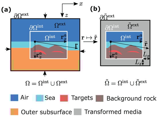
Figure 1. Illustration of the geometrical relation between (a) the physical model $\Omega ={\Omega }^{\mathrm{int}}\cup {\Omega }^{\mathrm{ext}}$ and (b) the compressed model $\tilde{\Omega }={\Omega }^{\mathrm{int}}\cup {\tilde{\Omega }}^{\mathrm{ext}}$. Here, ${\tilde{\Omega }}^{\mathrm{ext}}$ denotes the new boundary domain compressed from the original boundary region ${\Omega }^{\mathrm{ext}}$.

Taking partial derivatives on both sides of Equation (15) with respect to the transformed coordinates $(\tilde{x},\tilde{y},\tilde{z})$, we obtain the explicit expression of the inverse of Jacobian in Equation (3):

$${\mathbf{J}}^{-1}=\left(\begin{array}{ccc}{\mathsf{\Lambda }}_{x\tilde{x}}& 0& 0\\ 0& {\mathsf{\Lambda }}_{y\tilde{y}}& 0\\ 0& 0& {\mathsf{\Lambda }}_{z\tilde{z}}\end{array}\right)$$

(17)

with

$$\begin{array}{cc}\hfill {\mathsf{\Lambda }}_{v\tilde{v}}=& {\displaystyle \frac{\partial v}{\partial \tilde{v}}}\hfill \\ \hfill =& {\displaystyle \frac{a_{v}m}{L_v}}\widehat{H}\left({(\tilde{\mathbf{r}}-{\mathbf{r}}_v^a)}^T{\mathbf{n}}_v\right){\left({\displaystyle \frac{{(\tilde{\mathbf{r}}-{\mathbf{r}}_v^a)}^T{\mathbf{n}}_v}{L_v}}\right)}^{m-1}+1,v=x,y,z.\hfill \end{array}$$

(18)

It is readily seen that the Jacobian is non-singular throughout the entire computational domain, which will be reduced to an identity matrix in the interior region. Therefore, the transformed problem shown in Equation (4a)–(4c) is well defined over $\tilde{\Omega }$.

Before performing numerical simulations, it is useful to investigate the spatial variation in the equivalent material properties so as to predict the need of proper grid density. To draw a rough yet general conclusion for different model situations, we examine the following transformation tensor:

$$\mathbf{T}={\displaystyle \frac{\mathbf{J}{\mathbf{J}}^T}{det\left(\mathbf{J}\right)}}.$$

(19)

The underlying meaning of $\mathbf{T}$ becomes clear if we assume, without loss of generality, that the original electromagnetic coefficients are isotropic. Under this assumption, $\mathbf{T}$ directly reflects the heterogeneity and anisotropy that the coordinate transformation introduces in the transformed media. As an example, we show in Figure 2 the diagonal components of $\mathbf{T}$ at the slice $y=0 m$ on the model with dimensions $[-2 km,14 km]\times [-3 km,3 km]\times [-6 km,4 km]$. The interior domain is enclosed with dashed black lines and outside is the compressed boundary region. In the transformation function, m was set to 3 and scaling $a_i=25L_i,i=\pm x,\pm y,\pm z$ has been performed. This amounts to an original model with dimensions $[-52 km,64 km]\times [-53 km,53 km]\times [-81 km,29 km]$. From this figure, it is clear to see that a smaller computational domain comes at a cost of a stronger heterogeneous parameter distribution. Specifically, $a_i$ is directly related to the original scale of the computational domain. The factor $a_{i}m/L_i$ controls the parameter contrast while the factor m determines the spatial variation pattern. For the sake of numerical stability, the scaling factors $a_i/L_i$ and m should not be too large. We found with many tests that $m=3$ is suitable for MCSEM applications and therefore we used this value for all the experiments presented in this section.

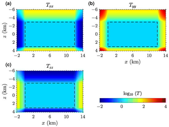
Figure 2. The diagonal component (a) $T_{xx}$, (b) $T_{yy}$ and (c) $T_{zz}$ of the transformation matrix $\mathbf{T}$ along $y=0 m$ defined in Equation (19). Dashed lines enclose the inner region.

3.1.1. 1D Marine Hydrocarbon Scenario

First, we validate the accuracy and practicability of our algorithm on 1D VTI models. The template consists of an air layer of $1\times {10}^{-7}\mathrm{S}/\mathrm{m}$, a seawater column of $3.2\mathrm{S}/\mathrm{m}$, a 1000 m thick sediment with a horizontal conductivity of $1\mathrm{S}/\mathrm{m}$ and a vertical conductivity of $0.2\mathrm{S}/\mathrm{m}$, and a 100 m thick isotropic layer of $0.01\mathrm{S}/\mathrm{m}$, followed by a deep basement with a horizontal conductivity of $0.5\mathrm{S}/\mathrm{m}$ and a vertical conductivity of $0.1\mathrm{S}/\mathrm{m}$. We consider two model variants that are a 1000 m deep-sea environment (Model I) and a 100 m shallow-water case (Model II), respectively. As an example, Figure 3a displays the geometry of Model I and the survey setup, and Figure 3b–d show the final refined meshes at frequency 0.25 Hz. For both models, the interior computational domain laterally encloses the survey region and vertically spans a 3000 m thick air layer and a 3000 m thick section from the sea surface to the deep subsurface, resulting in a total domain of size $[0 km,12 km]\times [-1 km,1 km]\times [-3 km,3 km].$ On both models, a horizontal electric dipole oriented with a $4.76°$ azimuth from the x-axis is located 50 m above the seabed. 24 inline receivers are positioned 0.05 m above the seafloor and along the source polarization direction with a lateral spacing of about 502 m to record the six electric and magnetic field components at frequencies $0.1$, $0.25$, $1$, and $10Hz$, respectively. For this survey geometry, the vertical component of the magnetic field $B_z$ becomes trivial. We used the same scaling coefficients $a_i=25L_i$ with $L_{\pm x}=2 km$, $L_{\pm y}=2 km$, $L_{+z}=1 km$, and $L_{-z}=3 km$ in both experiments. This gives rise to a final model size of dimensions $[-2 km,14 km]\times [-3 km,3 km]\times [-6 km,4 km]$.

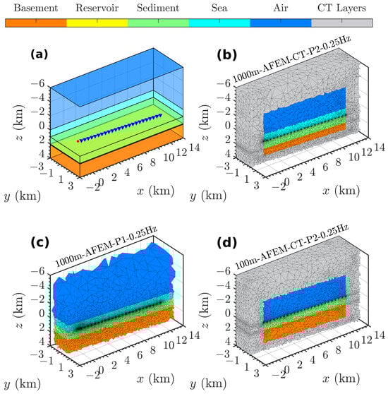
Figure 3. (a) Sketch of the 1D layered MCSEM model; (b) converged AFEM-CT-P2 mesh at 0.25 Hz for Model I; (c) converged AFEM-P1 mesh at 0.25 Hz for Model I; (d) converged AFEM-CT-P2 mesh at 0.25 Hz for Model II.

We executed the AFEM-CT-P2 algorithm for Model I at each frequency separately. Figure 4 depicts the comparison of the converged AFEM-CT-P2 results against the semi-analytical solutions [42]. For the sake of illustration, the errors for data below the noise floor (5 × 10⁻¹⁷ $\mathrm{V}$/$\mathrm{A}$$\mathrm{m}$ for the electric field and 5 × 10⁻²⁰ $\mathrm{T}$/$\mathrm{A}$$\mathrm{m}$ for the magnetic field) have been excluded from the error curves. It is evident from the figure that our AFEM-CT-P2 results agree well with the references. The maximum relative amplitude error among all data points is about 1.6% and the maximum phase difference is $0.8°$. Although not shown, we also computed the original forward problems on the physical model of the same scale as above. These results confirmed that the current model extent was sufficient for the 10 Hz data due to the rapid attenuation of high-frequency signals. However, at the three lower frequencies, significant boundary effects were observed, resulting in relative errors greater than 10% as the measuring points approach the outer boundary.

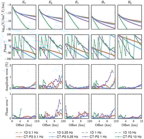
Figure 4. AFEM-CT-P2 results on the deep-sea Model I in comparison with the semi-analytical solutions.

To demonstrate the effectiveness of the presented algorithm, we have prepared a larger computational domain without the CT functionality. To make a justified comparison, we have run a few tests and picked the smallest-scale model which is able to render reasonable accuracy. The selected proper dimensions are $[-20 km,20 km,]\times [-20 km,20 km]\times [-70 km,40 km]$. The initial model discretization gives 1,787,181 tetrahedra and 11,323,722 DoFs with the second-order finite-element approximation. Apparently, the computational costs on the initial mesh with the traditional P2 discretization already exceed those on the final meshes with the AFEM-CT-P2 algorithm (Table 1). Therefore, further comparison was not executed. Instead, we switch to the lowest-order (P1) finite-element approximation. These converged AFEM-P1 results in comparison with the 1D solutions at each frequency are illustrated in Figure 5. We list the computational efforts for AFEM-CT-P2, AFEM-P2 and AFEM-P1 in Table 1. According to these statistics, it is evident that AFEM-CT-P2 shows decisive computational superiority. It reduces the number of DoFs by an order of magnitude compared to the conventional AFEM-P2 approach, while achieving a 63–76% reduction in computing time and a 14–47% reduction in memory usage versus the AFEM-P1 method.

Table 1. Comparison of computational costs for Model I using AFEM-CT-P2 versus AFEM-P2 and AFEM-P1. All experiments were conducted using 14 MPI processes with 4 OpenMP threads per process. ‘–’ denotes the process is not further executed.

	AFEM-CT-P2				AFEM-P1				AFEM-P2
	$\mathbf{16}\times \mathbf{6}\times \mathbf{10}$  km3				$\mathbf{40}\times \mathbf{40}\times \mathbf{110}$  km3				$\mathbf{40}\times \mathbf{40}\times \mathbf{110}$  km3
Frequency (Hz)	0.1	0.25	1	10	0.1	0.25	1	10	0.1	0.25	1	10
AFEM steps	6	7	6	8	13	13	13	14	0	0	0	0
Elements	373,568	375,050	218,112	192,130	3,298,259	2,909,945	2,655,371	2,674,748	1,787,181	1,787,181	1,787,181	1,787,181
DoFs	2,384,808	2,391,656	1,393,634	1,225,292	3,830,210	3,381,016	3,086,587	3,109,081	11,323,722	11,323,722	11,323,722	11,323,722
CPU time (s)	512	576	364	447	1665	1560	1495	1597	–	–	–	–
Memory (GB)	82	81	43	36	118	94	75	68	–	–	–	–

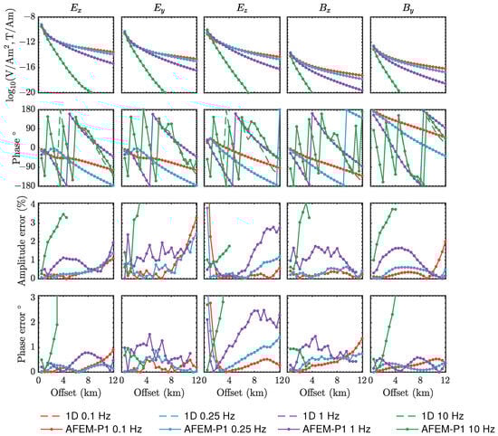
Figure 5. AFEM-P1 results on the deep-sea Model I without transformation in comparison with the semi-analytical solutions.

Following the same procedure, we examine the algorithm on the shallow-water Model II. In this experiment, we set the noise levels for the electric field and magnetic field to 5 × 10⁻¹⁶ $\mathrm{V}$/$\mathrm{A}$${\mathrm{m}}^2$ and 5 × 10⁻¹⁹ $\mathrm{T}$/$\mathrm{A}$$\mathrm{m}$, respectively. Figure 6 shows the nontrivial electromagnetic components at the four frequencies compared to the analytical solutions. Among all data points, we observe a maximum amplitude discrepancy of 4.8% in $E_z$ at 10 Hz at the farthest measuring location, where the signal amplitude is already very close to the noise floor. Apart from this data point, the relative amplitude deviations all remains below 1.2%. The maximum phase error is about $1.7°$. Based on the computational statistics given in Table 2, we highlight the capability of the CT technique in dealing with shallow-water models at low frequencies. Mesh accuracy at all acquisition frequencies can be ensured by about 350,000 to 490,000 tetrahedra, which correspond to 2 to 3 million DoFs for the second-order finite-element approximations. In contrast, this model becomes extremely challenging for the conventional FEM approach without the CT technique. By constraining the maximum aspect ratio to 1.4, the model with dimensions $[-30 km,30 km]\times [-30 km,30 km]\times [-70 km,40 km]$ is discretized into 7,549,120 elements, yielding 8,772,487 DoFs for the P1 formulation and 47,775,376 DoFs for the P2 case. It is apparent that both alternatives are inferior to the AFEM-CT-P2 approach, for which detailed comparisons are not conducted.

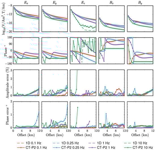
Figure 6. AFEM-CT-P2 results on the 100-m shallow-water Model II compared to the semi-analytical solutions.

Table 2. The computational costs using AFEM-CT-P2 for Model II versus AFEM-P1 and AFEM-P2. All experiments were finished on 14 MPI processes with 4 OpenMP threads each process. ‘–’ denotes the process is not further executed.

	AFEM-CT-P2				AFEM-P1				AFEM-P2
	$\mathbf{16}\times \mathbf{6}\times \mathbf{10}$  km3				$\mathbf{60}\times \mathbf{60}\times \mathbf{110}$  km3				$\mathbf{60}\times \mathbf{60}\times \mathbf{110}$  km3
Frequency (Hz)	0.1	0.25	1	10	0.1	0.25	1	10	0.1	0.25	1	10
AFEM steps	5	5	5	6	0	0	0	0	0	0	0	0
Elements	485,915	449,031	370,881	347,303	7,549,120	7,549,120	7,549,120	7,549,120	7,549,120	7,549,120	7,549,120	7,549,120
DoFs	3,100,168	2,864,300	2,366,002	2,214,098	8,772,487	8,772,487	8,772,487	8,772,487	47,775,376	47,775,376	47,775,376	47,775,376
CPU time (s)	708	667	605	677	–	–	–	–	–	–	–	–
Memory (GB)	121	104	84	72	–	–	–	–	–	–	–	–

3.1.2. 3D Anticline Trap with Bathymetry

Based on the above validation, we now utilize this algorithm to analyze a 3D bathymetric model with a local anticline trap [7,43]. While comprehensive studies are essential to fully understand the impact of complex electrical anisotropy, this work focuses on the anticline scenario to demonstrate the capability of our approach in handling generally anisotropic conductivity within complex geological settings. Figure 7 displays the geometry and initial mesh of the computational domain. The solid black lines mark the boundaries of the interior subdomain. Outside the black lines are the transformed regions. In the target domain, the water depth varies from about 600 m to about 1200 m. A 3000 m thick air layer of $1\times {10}^{-7}\mathrm{S}/\mathrm{m}$ was appended on top of the sea surface. The hydrocarbon reservoir was modeled as a local 3D resistive body of $0.01\mathrm{S}/\mathrm{m}$ and dimensions $5 km \times 5 km \times 0.1 km$, trapped in a local symmetric anticline structure of $\left|\beta \right|=20°$ dip formed by two limbs of dimensions $4 km \times 6 km \times 1.5 km$. The rest of the rugged sediment is assumed to be vertically transversely isotropic with a horizontal conductivity of $1\mathrm{S}/\mathrm{m}$ and a vertical conductivity of $0.25\mathrm{S}/\mathrm{m}$. A VTI basement is underlain with a horizontal conductivity of $1\mathrm{S}/\mathrm{m}$ and a vertical conductivity of $0.2\mathrm{S}/\mathrm{m}$. In the transformed domain, the deep basement was compressed to 1 km thickness. The boundary effect along the other directions was taken into account by 2 km thick layers surrounding the vertical boundaries and a 3 km thick layer on top of the air space with equivalent materials. Again, the transformation scaling $a_i=25L_i$ was utilized.

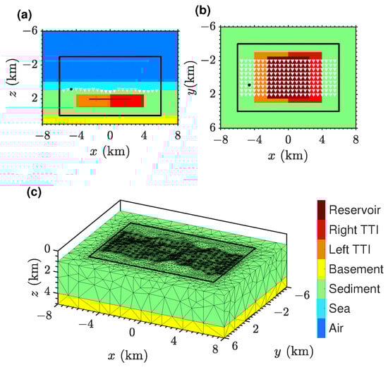
Figure 7. Panels (a,b) show the plane view of the 3D bathymetric model at $y=0 m$ and $z=2050 m$, respectively; (c) the initial discretization of the subsurface. The black dot and white triangles in (a,b) mark the transmitter’s and receivers’ positions, respectively.

We deployed a dense acquisition array consisting of 207 receivers arranged in a $23\times 9$ grid with each station spaced $500 m$ apart (see Figure 7b) to record the EM responses. Due to the bathymetry, the vertical positions of the receivers vary from about 644 m to about 1197 m. An x-directed horizontal electric dipole is situated at $(-4600 m,0,880 m)$, roughly $50 m$ above the seabottom. The transmission frequencies were set to 0.1, 0.25, 1, and 10 Hz.

We apply the AFEM-CT-P2 procedure to compute the TTI model (referred to as TTIA) responses at the four frequencies separately. To analyze the impact of electrical anisotropy, the background model excluding the anticline and reservoir bodies (named by VTIB) as well as the model without the anticline (named by VTIA) were also computed. Given field measurements are often contaminated with different sources of errors, we conduct a realistic sensitivity analysis according to Brown et al. [5]:

$$S_{F_i}={\displaystyle \frac{|F_i|-|F^{\mathrm{VTIB}}|}{F_i^{\mathrm{noise}}}},i=x,y,$$

(20)

where $F_i^{\mathrm{noise}}$ is the estimated data uncertainty for each horizontal component, reading

$$F_{x,y}^{\mathrm{noise}}=\sqrt{({\alpha }^2+{(cos\varphi -1)}^2)|F_{x,y}{|}^2+{sin}^2\varphi {\left|F_{y,x}\right|}^2+e^2}.$$

(21)

As described in Equation (21), this formulation accounts for three error sources: the relative error in the measurements ($\alpha$), the rotation uncertainty ($\varphi$), and the noise floor (e). In this experiment, we set $\alpha =0.03$, $\varphi =2°$, the noise floor for the electric and magnetic field to 1 × 10⁻¹⁶ $\mathrm{V}$/$\mathrm{A}$${\mathrm{m}}^2$ and 1 × 10⁻¹⁹ $\mathrm{T}$/$\mathrm{A}$$\mathrm{m}$, respectively. Figure 8 and Figure 9 show the resolution of the anomalous signals with respect to the data uncertainty for each horizontal data component on model VTIA and TTIA, respectively. It is clearly seen that the effective sensitivity of the composite responses of the anticline and reservoir is much weaker than that in the VTI case. Given the weak responses, an accurate forward operator becomes essential for imaging the challenging anticline traps.

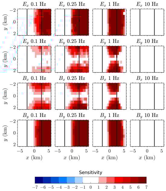
Figure 8. The resolution of anomalous signals on model VTIA with respect to the data uncertainty. The black lines outline the horizontal extent of the oil reservoir.

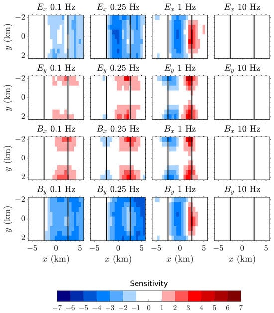
Figure 9. The resolution of anomalous signals on model TTIA with respect to the data uncertainty.

3.2. Application to High-Resolution Models

3.2.1. Depth-Varying Seawater Conductivity Profile

Next, we examine the potential of the CT technique in handling complex, high-resolution models. Due to the combined effects of temperature, salinity, and pressure, seawater conductivity can vary with depth [44]. Given the limited spatial extent of MCSEM surveys, such vertical variations in seawater conductivity may influence electromagnetic responses, thereby highlighting the need for further investigation. To explore this effect, we design a simplified seawater conductivity profile following Zheng et al. [44], where conductivity decays exponentially from about 5.6 S/m at the sea surface to about 3.4 S/m at the seabottom of 1000 m. The depth-varying conductivity profile is discretized into 50 m thick layers. The conductivity of each layer is calculated as the average conductivity across the layer’s thickness (see Figure 10). The model setup of the subsurface is identical to that in the 1D benchmark described in the last section.

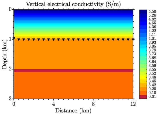
Figure 10. Sketch of the depth-varying seawater conductivity profile. The black dot and triangles mark the transmitter’s and receivers’ positions, respectively.

We apply a composite coordinate transformation to this model. First, a stretching function is designed to expand the vertical spacing between layers beneath the sea surface by a factor of six. Then, a compression function, similar to Equation (15) but with $L_{\pm x}=3 km$ and $L_{\pm y}=3 km$, is composited to squeeze the boundary subdomain. This yields a transformed model with dimensions $18 \mathrm{k}\mathrm{m} \times 8 \mathrm{k}\mathrm{m} \times 30 \mathrm{k}\mathrm{m}$. Figure 11 depicts the numerical results in comparison with the semi-analytical solutions. It is seen that the AFEM-CT-P2 results match well with the references with a maximum amplitude error less than $1.6\%$ and phase error $0.5°$. However, modeling such continuously fine layers using standard finite-element schemes with unstructured grids becomes computationally intensive. For example, an initial tetrahedralization of this profile shaped into a 3D computational domain of size $16 km \times 6 km \times 11 km$ yields over 3.2 million cells. In contrast, the AFEM-CT-P2 scheme is designed to mitigate the geometrical disparity between structures of different scales. The procedure converges to accurate solutions at all working frequencies with no more than 525,379 cells and 3,346,976 DoFs, which corresponds to only 16.4% of the elements needed in the conventional methods.

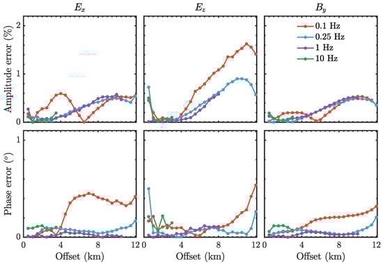
Figure 11. AFEM-CT-P2 results on the seawater conductivity profile in comparison with the semi-analytical solutions.

To evaluate the impact of depth-varying seawater conductivity on the electromagnetic responses, we compare the fields with the responses of a constant seawater column of 3.42 S/m, namely the conductivity measured at receiver positions. To account for realistic environmental conditions, an optimistic noise floor 1 × 10⁻¹⁵ $\mathrm{V}$/$\mathrm{A}$${\mathrm{m}}^2$ and 1 × 10⁻¹⁸ $\mathrm{T}$/$\mathrm{A}$$\mathrm{m}$ have been assumed for the electric and magnetic field, respectively. It is seen from Figure 12 that the vertical variation in seawater conductivity most strongly affects the electromagnetic field at 0.1 Hz. A moderate impact is observed at 0.25 Hz within a short transmitter–receiver offset less than 4 km. In contrast, trivial influence is found at frequencies higher than 1 Hz. This frequency-dependent behavior seems reasonable since lower-frequency signals penetrate deeper and are more sensitive to the spatial variation in the conductivity profile. Whereas higher-frequency signals are primarily influenced by the local environment near the source and receivers. Among the EM field components, $E_x$ shows strong sensitivity to changes in the seawater conductivity, as it is affected by broad, horizontally distributed current systems. In contrast, $E_z$ is less affected, as it is primarily governed by localized vertical current paths.

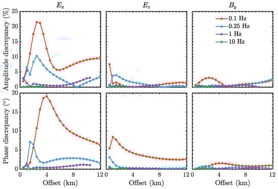
Figure 12. The difference in field responses between the depth-varying seawater conductivity profile and the constant conductivity seawater column.

3.2.2. Marlim R3D

Finally, we apply the CT approach to a real-world MCSEM model. Marlim R3D (MR3D) is an open-source and realistic geoelectric model developed for simulating CSEM responses of postsalt turbiditic reservoirs along the Brazilian offshore margin [45]. The MR3D resistivity model is initially defined on a uniform hexahedral mesh with the target region comprising nearly 90 million cells. Reconstructing such a high-resolution conductivity distribution using numerical methods based on unstructured mesh discretization is computationally demanding. Rochlitz et al. [37] and Werthmüller et al. [46] conducted a comprehensive study on this model with a robust mesh generation and resistivity interpolation workflow tailored to tetrahedral meshes. We utilize this preprocessing procedure to construct the discretized conductivity model. Prior to that, the CT approach is applied to vertically stretch the subdomain beneath the sea surface by a factor of six. A gradual global refinement is then performed over the target region, generating three successively finer unstructured meshes. Throughout this process, the initial triangulation of known geological interfaces is preserved to ensure geometrical consistency. The coarsest mesh comprises 1,060,715 elements, the intermediate mesh comprises 1,182,126 elements, and the finest mesh comprises 3,120,950 elements. For each mesh, the conductivity distribution is re-interpolated accordingly (see Figure 13). Each model is individually solved using the FEM-CT-P2 approach. We note that although a much coarser discretization similar to that in Rochlitz et al. [37] and Werthmüller et al. [46] could have been reused, we chose to construct new meshes in order to better represent the complexity of the MR3D model, and, furthermore, to analyze the sensitivity of the electromagnetic fields to finely resolved geological bodies. We employ the AMS-preconditioned FGMRES method to solve the three models. Despite the strong heterogeneity and anisotropy, which typically increase the condition number of the system matrix [47], the solver consistently converges within 17–20 iterations to a tolerance of ${10}^{-9}$ across all experiments in the frequency range of 0.125–1.25 Hz. Its performance is comparable to the non-transformed cases with different meshes, which converge in 17–19 iterations.

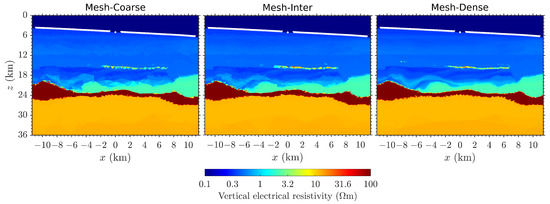
Figure 13. Slices of the interpolated transformed MR3D model at different levels of mesh refinement. White dot and triangles indicate the source location and measurement positions.

To illustrate the results, Figure 14 and Figure 15 depict the comparison of the computed inline and broadside components on the three meshes at frequencies of 0.25 and 1Hz, respectively, with references on the hexahedral mesh [45]. For additional verification, the results from Rochlitz et al. [37] are also included to help identify the source of any discrepancies. We have excluded the errors for data below the noise floor (1 × 10⁻¹⁶ $\mathrm{V}$/$\mathrm{A}$${\mathrm{m}}^2$ for the electric field) from the error curves. The results reveal that the coarsest mesh deviates most significantly from the reference solution. This may result from insufficient mesh density to ensure the numerical accuracy for the equivalent materials. In contrast, the moderate and finest meshes produce results with similar levels of accuracy, indicating that additional mesh refinement, or accordingly, a further increase in model resolution yields marginal improvements. Nevertheless, a residual discrepancy of approximately 10% persists [46]. The observed non-negligible difference is likely due to deviations in how irregular geometries are represented and how boundary domain extensions are treated in different implementations.

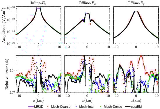
Figure 14. Comparison of the computed electric field components on the three meshes at 0.25 Hz with the reference ‘MR3D’ [45].

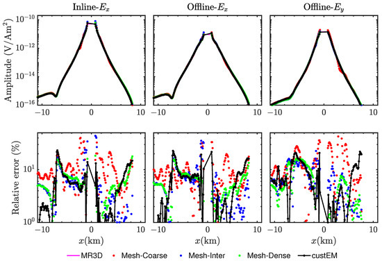
Figure 15. Comparison of the computed electric field components on the three meshes at 1 Hz with the reference ‘MR3D’ [45].

4. Conclusions

We have developed a parallel adaptive high-order finite-element framework for large-scale 3D marine controlled-source electromagnetic modeling in the frequency domain. Although high-order finite-element methods offer high accuracy and robustness, their application to 3D MCSEM problems remains constrained for models involving thin layers or regional multi-scale heterogeneities. To address this challenge, this work introduced a coordinate transformation approach based on the form invariance of Maxwell’s equations. By designing a problem-specific spatial mapping, the structural complexity and scale contrasts among different structures can be effectively reduced. As a trade-off, the transformation yields a new formulation characterized by equivalent anisotropic materials, while still preserving the original mathematical structure of Maxwell’s equations. This allows the transformed problem to be solved using standard high-order finite-element solvers. Since the new electromagnetic parameters become spatially varying and anisotropic, we employed a goal-oriented mesh refinement strategy to ensure accurate modeling of the complex field behavior in target regions.

The 1D benchmark tests demonstrate that our solver performs competitively in deep-sea environments and offers clear advantages over the traditional approach in shallow-water settings and scenarios with depth-dependent conductivity variations. The practicality of our approach was further illustrated using a TTI model with rugged seafloor topography. The resulting sensitivity analysis highlights the critical importance of using an accurate forward solver to resolve the weak electromagnetic responses associated with anticline traps. Finally, we revisited the MR3D model. The convergence study inferred that high-resolution models may not be fully resolved due to the diffusive behavior of low-frequency electromagnetic fields. This suggests that MCSEM inversion workflows could benefit from adaptive model parameterization to balance the resolution and computational efficiency.

Although only MCSEM applications were considered here, this method can be naturally applied to plane wave EM modeling. However, it is worth pointing out that the CT approach does not inherently improve the simulation accuracy. Rather, it alleviates geometrical complexity at the cost of increased contrast in material properties. This trade-off could present further challenges for iterative solvers. Nevertheless, by employing a robust Maxwell solver such as the AMS-preconditioned FGMRES, we observe no significant difficulties in solving the resulting system of equations.

References

- Key, K. Marine electromagnetic studies of seafloor resources and tectonics. Surv. Geophys. 2012, 33, 135–167. [Google Scholar] [CrossRef]
- Zhdanov, M.S.; Endo, M.; Yoon, D.; Čuma, M.; Mattsson, J.; Midgley, J. Anisotropic 3D inversion of towed-streamer electromagnetic data: Case study from the Troll West Oil Province. Interpretation 2014, 2, SH97–SH113. [Google Scholar] [CrossRef]
- Zhdanov, M.S.; Endo, M.; Cox, L.H.; Čuma, M.; Linfoot, J.; Anderson, C.; Black, N.; Gribenko, A.V. Three-dimensional inversion of towed streamer electromagnetic data. Geophys. Prospect. 2014, 62, 552–572. [Google Scholar] [CrossRef]
- Newman, G.A.; Commer, M.; Carazzone, J.J. Imaging CSEM data in the presence of electrical anisotropy. Geophysics 2010, 75, F51–F61. [Google Scholar] [CrossRef]
- Brown, V.; Hoversten, M.; Key, K.; Chen, J. Resolution of reservoir scale electrical anisotropy from marine CSEM data. Geophysics 2012, 77, E147–E158. [Google Scholar] [CrossRef]
- Cook, A.E.; Anderson, B.I.; Malinverno, A.; Mrozewski, S.; Goldberg, D.S. Electrical anisotropy due to gas hydrate-filled fractures. Geophysics 2010, 75, F173–F185. [Google Scholar] [CrossRef]
- Jaysaval, P.; Shantsev, D.V.; de la Kethulle de Ryhove, S.; Bratteland, T. Fully anisotropic 3-D EM modelling on a Lebedev grid with a multigrid pre-conditioner. Geophys. J. Int. 2016, 207, 1554–1572. [Google Scholar] [CrossRef]
- Li, J.; Liu, Y.; Han, B.; Lu, J. Impacts of complex geological structures on marine controlled-source electromagnetic responses. J. Appl. Geophys. 2020, 180, 104126. [Google Scholar] [CrossRef]
- Peng, R.; Hu, X.; Li, J.; Liu, Y. Finite element simulation of 3-D marine controlled source electromagnetic fields in anisotropic media with unstructured tetrahedral grids. Pure Appl. Geophys. 2020, 177, 4871–4882. [Google Scholar] [CrossRef]
- Jaysaval, P.; Shantsev, D.; de la Kethulle de Ryhove, S. Fast multimodel finite-difference controlled-source electromagnetic simulations based on a Schur complement approach. Geophysics 2014, 79, E315–E327. [Google Scholar] [CrossRef]
- Zhdanov, M.; Lee, S.; Yoshioka, K. Integral equation method for 3D modeling of electromagnetic fields in complex structures with inhomogeneous background conductivity. Geophysics 2006, 71, G333–G345. [Google Scholar] [CrossRef]
- Jahandari, H.; Farquharson, C. Finite-volume modelling of geophysical electromagnetic data on unstructured grids using potentials. Geophys. J. Int. 2015, 202, 1859–1876. [Google Scholar] [CrossRef]
- Cai, H.; Xiong, B.; Han, M.; Zhdanov, M. 3D controlled-source electromagnetic modeling in anisotropic medium using edge-based finite element method. Comput. Geosci. 2014, 73, 164–176. [Google Scholar] [CrossRef]
- Ren, Z.; Kalscheuer, T.; Greenhalgh, S.; Maurer, H. A finite-element-based domain-decomposition approach for plane wave 3D electromagnetic modeling. Geophysics 2014, 79, E255–E268. [Google Scholar] [CrossRef]
- Grayver, A.V.; Kolev, T.V. Large-scale 3D geoelectromagnetic modeling using parallel adaptive high-order finite element method. Geophysics 2015, 80, E277–E291. [Google Scholar] [CrossRef]
- Zhou, F.; Chen, H.; Tang, J.; Zhang, Z.; Yuan, Y.; Wu, Q. A comparison of A-phi formulae for three-dimensional geo-electromagnetic induction problems. J. Geophys. Eng. 2022, 19, 630–649. [Google Scholar] [CrossRef]
- Schwarzbach, C.; Börner, R.U.; Spitzer, K. Three-dimensional adaptive higher order finite element simulation for geo-electromagnetics—A marine CSEM example. Geophys. J. Int. 2011, 187, 63–74. [Google Scholar] [CrossRef]
- Qin, C.; Li, H.; Li, H.; Zhao, N. High-order finite-element forward-modeling algorithm for the 3D borehole-to-surface electromagnetic method using octree meshes. Geophysics 2024, 89, F61–F75. [Google Scholar] [CrossRef]
- Grayver, A.V.; Bürg, M. Robust and scalable 3-D geo-electromagnetic modelling approach using the finite element method. Geophys. J. Int. 2014, 198, 110–125. [Google Scholar] [CrossRef]
- Castillo-Reyes, O.; de la Puente, J.; García-Castillo, L.E.; Cela, J.M. Parallel 3-D marine controlled-source electromagnetic modelling using high-order tetrahedral Nédélec elements. Geophys. J. Int. 2019, 219, 39–65. [Google Scholar] [CrossRef]
- Ren, Z. New Developments in Numerical Modeling of Broadband Geo-Electromagnetic Fields. Ph.D. Thesis, ETH Zurich, Zurich, Switzerland, 2012. [Google Scholar]
- Ren, Z.; Kalscheuer, T.; Greenhalgh, S.; Maurer, H. A hybrid boundary element-finite element approach to modeling plane wave 3D electromagnetic induction responses in the Earth. J. Comput. Phys. 2014, 258, 705–717. [Google Scholar] [CrossRef]
- Bérenger, J.P. Perfectly Matched Layer (PML) for Computational Electromagnetics, 1st ed.; Synthesis Lectures on Computational Electromagnetics; Springer: Cham, Switzerland, 2007; pp. 1–117. [Google Scholar]
- Schwarzbach, C. Stability of Finite Element Solutions to Maxwell’s Equations in Frequency Domain. Ph.D. Thesis, Technische Universität Bergakademie Freiberg, Freiberg, Germany, 2009. [Google Scholar]
- Li, G.; Li, Y.; Han, B.; Liu, Z. Application of the perfectly matched layer in 3-D marine controlled-source electromagnetic modelling. Geophys. J. Int. 2018, 212, 333–344. [Google Scholar] [CrossRef]
- Liu, J.; Xiao, X.; Tang, J.; Ren, Z.; Huang, X.; Zhang, J. Fast 3-D controlled-source electromagnetic modeling combining UPML and rational Krylov method. IEEE Geosci. Remote Sens. Lett. 2022, 19, 3006505. [Google Scholar] [CrossRef]
- de la Kethulle de Ryhove, S.; Mittet, R. 3D marine magnetotelluric modeling and inversion with the finite-difference time-domain method. Geophysics 2014, 79, E269–E286. [Google Scholar] [CrossRef]
- Pendry, J.B.; Schurig, D.; Smith, D.R. Controlling electromagnetic fields. Science 2006, 312, 1780–1782. [Google Scholar] [CrossRef] [PubMed]
- Ozgun, O.; Kuzuoglu, M. Form invariance of Maxwell’s equations: The pathway to novel metamaterial specifications for electromagnetic reshaping. IEEE Antennas Propag. Mag. 2010, 52, 51–65. [Google Scholar] [CrossRef]
- Shyroki, D.M.; Ivinskaya, A.M.; Lavrinenko, A.V. Free-space squeezing assists perfectly matched layers in simulations on a tight domain. IEEE Antennas Wirel. Propag. Lett. 2010, 9, 389–392. [Google Scholar] [CrossRef][Green Version]
- Kamm, J.; Becken, M.; Abreu, R. Electromagnetic modelling with topography on regular grids with equivalent materials. Geophys. J. Int. 2020, 220, 2021–2038. [Google Scholar] [CrossRef]
- Chen, H.; Xiong, B.; Lu, Y.; Jiang, Q.; Huang, L.; Zhou, S. Three-dimensional modeling of marine controlled source electromagnetic using a new high-order finite element method with an absorption boundary condition. IEEE Trans. Geosci. Remote Sens. 2023, 61, 2001909. [Google Scholar] [CrossRef]
- Weidelt, P. 3D conductivity models: Implications of electrical anisotropy. In Three-Dimensional Electromagnetics; Oristaglio, M., Spies, B., Eds.; Society of Exploration Geophysicists: Houston, TX, USA, 1999. [Google Scholar]
- Kottke, C.; Farjadpour, A.; Johnson, S.G. Perturbation theory for anisotropic dielectric interfaces, and application to subpixel smoothing of discretized numerical methods. Phys. Rev. E 2008, 77, 036611. [Google Scholar] [CrossRef]
- Schurig, D.; Pendry, J.B.; Smith, D.R. Calculation of material properties and ray tracing in transformation media. Opt. Express 2006, 14, 9794–9804. [Google Scholar] [CrossRef] [PubMed]
- Li, J.; Huang, Y.; Yang, W. An adaptive edge finite element method for electromagnetic cloaking simulation. J. Comput. Phys. 2013, 249, 216–232. [Google Scholar] [CrossRef]
- Rochlitz, R.; Seidel, M.; Börner, R.U. Evaluation of three approaches for simulating 3-D time-domain electromagnetic data. Geophys. J. Int. 2021, 227, 1980–1995. [Google Scholar] [CrossRef]
- Ren, Z.; Kalscheuer, T.; Greenhalgh, S.; Maurer, H. A goal-oriented adaptive finite-element approach for plane wave 3-D electromagnetic modelling. Geophys. J. Int. 2013, 194, 700–718. [Google Scholar] [CrossRef]
- Anderson, R.; Andrej, J.; Barker, A.; Bramwell, J.; Camier, J.S.; Cerveny, J.; Dobrev, V.; Dudouit, Y.; Fisher, A.; Kolev, T.; et al. MFEM: A modular finite element methods library. Comput. Math. Appl. 2021, 81, 42–74. [Google Scholar] [CrossRef]
- Si, H. TetGen, a Delaunay-based quality tetrahedral mesh generator. ACM Trans. Math. Softw. 2015, 41, 1–36. [Google Scholar] [CrossRef]
- Amestoy, P.R.; de la Kethulle de Ryhove, S.; L’Excellent, J.Y.; Moreau, G.; Shantsev, D.V. Efficient use of sparsity by direct solvers applied to 3D controlled-source EM problems. Comput. Geosci. 2019, 23, 1237–1258. [Google Scholar] [CrossRef]
- Streich, R.; Becken, M. Sensitivity of controlled-source electromagnetic fields in planarly layered media. Geophys. J. Int. 2011, 187, 705–728. [Google Scholar] [CrossRef][Green Version]
- Davydycheva, S.; Frenkel, M.A. The impact of 3D tilted resistivity anisotropy on marine CSEM measurements. Lead. Edge 2013, 32, 1374–1381. [Google Scholar] [CrossRef]
- Zheng, Z.; Fu, Y.; Liu, K.; Xiao, R.; Wang, X.; Shi, H. Three-stage vertical distribution of seawater conductivity. Sci. Rep. 2018, 8, 9916. [Google Scholar] [CrossRef]
- Correa, J.L.; Menezes, P.T.L. Marlim R3D: A realistic model for controlled-source electromagnetic simulations — Phase 2: The controlled-source electromagnetic data set. Geophysics 2019, 84, E293–E299. [Google Scholar] [CrossRef]
- Werthmüller, D.; Rochlitz, R.; Castillo-Reyes, O.; Heagy, L. Towards an open-source landscape for 3-D CSEM modelling. Geophys. J. Int. 2021, 227, 644–659. [Google Scholar] [CrossRef]
- Liu, Z.; Yao, H.; Wang, F. Performance investigations of auxiliary-space Maxwell solver preconditioned iterative algorithm for controlled-source electromagnetic induction problems with electrical anisotropy. Geophys. Prospect. 2024, 72, 2861–2879. [Google Scholar] [CrossRef]
Disclaimer/Publisher’s Note: The statements, opinions and data contained in all publications are solely those of the individual author(s) and contributor(s) and not of MDPI and/or the editor(s). MDPI and/or the editor(s) disclaim responsibility for any injury to people or property resulting from any ideas, methods, instructions or products referred to in the content. |
© 2025 by the authors. Licensee MDPI, Basel, Switzerland. This article is an open access article distributed under the terms and conditions of the Creative Commons Attribution (CC BY) license (https://creativecommons.org/licenses/by/4.0/).