Research on 3D Modeling Method of Tunnel Surrounding Rock Structural Planes Based on B-Spline Interpolation

Abstract

To address the limitations of traditional tunnel structural plane modeling—such as low automation, insufficient smoothness, and poor adaptability to real construction environments—this study proposes a novel three-dimensional (3D) modeling framework based on B-spline interpolation combined with deep learning. The method first employs YOLOv5 for rapid detection of structural regions and DeepLabV3+ for precise boundary segmentation, followed by skeleton extraction and coordinate transformation to obtain spatial structural traces. Finally, B-spline interpolation is applied across multiple tunnel sections to construct continuous 3D surfaces. In model training and testing, the segmentation network achieved an F1 score of 94.01%, and the final modeling accuracy demonstrated a mean relative error (MRE) below 2.5%, confirming the reliability of the geometric reconstruction. Additionally, the proposed method was applied to excavation face images from the Paiyashan Tunnel, where multiple structural surfaces were successfully reconstructed in 3D, validating the approach’s applicability and robustness in real geological conditions. Compared to traditional triangulated or linear surface methods, the proposed approach achieves higher smoothness, better geological continuity, and improved automation, making it suitable for real-world geotechnical applications.

1. Introduction

In underground engineering, particularly tunnel construction, the stability of surrounding rock masses plays a critical role in ensuring both construction safety and long-term operational reliability [1]. Structural planes—including joints, fractures, bedding planes, and faults—are naturally occurring discontinuities that strongly influence the mechanical behavior, deformation patterns, and failure mechanisms of rock masses [2,3]. Accurate and efficient identification and three-dimensional (3D) reconstruction of these structural planes have therefore become focal points in geotechnical modeling and digital geological analysis [4,5].

Traditional methods such as geological compass measurements and manual sketching are limited by on-site constraints like poor lighting, narrow working space, and humidity, leading to inefficiencies and high labor costs [6,7,8]. Recent advances in computer vision and deep learning offer promising alternatives [9,10,11]. Object detection and semantic segmentation techniques have been increasingly applied to geological image analysis and tunnel face interpretation [12,13,14]. Meanwhile, 3D reconstruction methods such as structure-from-motion (SfM), laser scanning, and structured light scanning have also been explored [15,16,17]. However, these techniques often rely on expensive equipment and are sensitive to environmental conditions, which limits their field deployment in tunnel engineering.

Existing 3D modeling methods include triangulated irregular networks (TINs) [18], linear surface interpolation [19], cubic splines [20], NURBS [21], and Delaunay triangulation [22]. In contrast, B-spline interpolation offers high-order continuity, strong local controllability, and superior geometric fidelity, making it especially suitable for modeling geologically complex and fragmented surfaces. Belhachmi et al. proposed a spline-based regularization method for complex geological body reconstruction, demonstrating its effectiveness in representing stratigraphic boundaries and discontinuities with high smoothness and accuracy [23]. Peng et al. applied high-order B-spline basis functions in the material point method to simulate the deformation and failure of layered rock masses, significantly improving computational precision [24]. Despite these advantages, few studies have integrated B-spline modeling with automated feature recognition under practical tunnel conditions. Most existing works either focus solely on feature extraction or apply B-splines in idealized scenarios without addressing real-world data uncertainties, automation requirements, or computational efficiency.

To bridge this gap, this study proposes a fully automated 3D modeling framework that combines YOLOv5-based object detection [25], DeepLabV3+-based semantic segmentation [26], and B-spline surface interpolation. Validated using real-world images from the Paiyashan Tunnel, the proposed method achieves high segmentation accuracy and precise surface reconstruction. Compared to conventional techniques, it offers an improved balance between accuracy, efficiency, and adaptability in challenging field conditions.

2. Intelligent Identification of Structural Surfaces

As a critical geometric input for surrounding rock modeling, accurate identification of structural surfaces is fundamental to achieving digital reconstruction of tunnel geology. To improve both recognition efficiency and accuracy, this study proposes an automatic structural surface identification method based on deep learning, which integrates YOLOv5 and DeepLabV3+ models. The overall process consists of three stages: (1) object detection to localize the structural surface region; (2) semantic segmentation to extract precise boundaries; and (3) skeletonization to obtain the central axis of the surface, providing geometric input for subsequent 3D reconstruction.

2.1. Structural Surface Detection Using YOLOv5

YOLOv5 is a lightweight single-stage object detection network known for its fast inference speed and high accuracy. To enhance the model’s robustness and generalization capability, a heterogeneous dataset containing 1260 images was constructed, incorporating tunnel face images, natural rock outcrops, and concrete surface cracks (see Figure 1). The dataset was divided into training, validation, and testing sets at an 8:1:1 ratio.

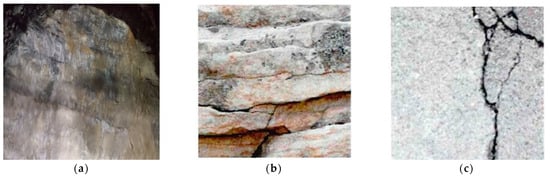
Figure 1. Examples of heterogeneous structural surface images. (a) Tunnel face images; (b) natural rock outcrops; (c) concrete surface cracks.

All images were resized to 640 × 640 pixels and denoised using Gaussian and bilateral filters. Structural surface regions were manually annotated using the LabelImg tool. During training, the Complete IoU (CIoU) loss function and a cosine annealing learning rate scheduler were employed to enhance convergence stability and mitigate overfitting. The YOLOv5 model was trained with a batch size of 16 and an initial learning rate of 0.001, using the Adam optimizer for a maximum of 150 epochs. Early stopping was implemented based on validation loss plateauing for 10 consecutive epochs. To improve generalization under varying geological textures and lighting conditions, a range of data augmentation techniques was applied, including random horizontal flipping, rotation (±15°), scaling (±10%), color jittering, and brightness perturbation. The training was conducted on an NVIDIA RTX 3090 GPU using PyTorch 1.13, with a total training time of approximately 5 h. The default anchor boxes provided by YOLOv5 were used throughout. An example of the detection results is shown in Figure 2.

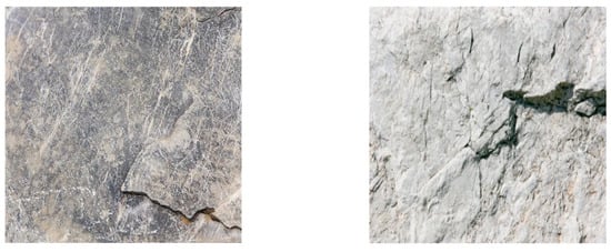
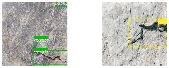
Figure 2. Structural surface localization results using YOLOv5.

2.2. Semantic Segmentation Using DeepLabV3+

To further improve the accuracy of boundary extraction, DeepLabV3+ was employed to perform pixel-level segmentation within the regions detected by YOLOv5. This model uses an Xception encoder and atrous spatial pyramid pooling (ASPP) to capture multi-scale contextual information, making it well-suited for segmenting complex textures and blurry edges.

Prior to training, all images and mask labels were resized to 512 × 512 pixels. Data augmentation techniques such as rotation, scaling, and brightness perturbation were applied to enhance the model’s robustness to illumination and shape variation. The network was trained using the cross-entropy loss function and optimized via the Adam optimizer, with early stopping to prevent overfitting. The final model achieved an F1 score of 94.01% on the test set, indicating strong segmentation performance. In addition to the F1 score of 94.01%, we evaluated model performance using precision and recall curves, as shown in Figure 3. These demonstrate the stable convergence and improved classification ability of the segmentation network over training epochs. A representative result is presented in Figure 4.

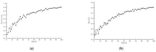
Figure 3. Precision and recall curves of the segmentation model. (a) Relationship between model precision and number of iterations.; (b) Relationship between model recall and number of iterations.

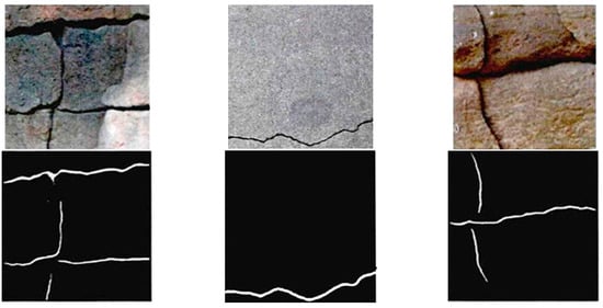
Figure 4. Structural surface boundary segmentation results using DeepLabV3+.

2.3. Skeleton Extraction and Geometric Transformation

As the segmentation output typically consists of regions with certain widths, they cannot be directly used for geometric modeling. To address this, the skeleton of the segmented structural surfaces was extracted using the skeletonize () function from the skimage.morphology module in the Python 3.12 scikit-image library. This morphological operation converts the segmented regions into single-pixel-wide skeleton lines, accurately preserving the geometric shape of the structures for subsequent modeling.

3. Coordinate Transformation of Structural Plane Information

To accurately reconstruct structural planes in 3D space, it is essential to convert their two-dimensional image information into physical spatial coordinates. This process involves three key steps: coordinate system definition, image preprocessing, and coordinate sampling, which together establish a geometric foundation for subsequent surface modeling.

3.1. Establishment of a Spatial Coordinate System

The coordinate system established in this study is a local project-specific system aligned with the tunnel cross-section design. It is not referenced to a global geodetic coordinate system such as WGS84 or UTM. The origin and axis directions are defined based on known geometric markers in the image (yellow origin and green scale bar), with a physical-to-pixel conversion ratio derived from field measurements. The expected positioning accuracy of the coordinate origin is within ±5 pixels, which corresponds to an average physical deviation of less than 2 cm in both X and Z directions, defined as follows:

X-axis: Defined by the line connecting the intersection points of the lower arcs in the inner contour drawn using the three-center circle method. The direction to the right is taken as positive. This axis represents the lateral position of the tunnel cross-section.

Z-axis: Defined as the perpendicular bisector of the X-axis line, with the upward direction being positive. It indicates the vertical elevation of the cross-section.

Y-axis: Oriented in the tunnel excavation direction, with forward advancement as positive. This axis describes the spatial location of the structural plane along the tunnel’s longitudinal direction.

This coordinate system not only conforms to conventional tunnel engineering practices but also facilitates data sampling and 3D reconstruction.

3.2. Image Preprocessing and Structural Feature Extraction

To automate the extraction of coordinate and structural plane information from tunnel cross-section drawings, a color-based recognition procedure was developed. As illustrated in Figure 5a, which is a simulated schematic based on actual tunnel design drawings created using AutoCAD 2017 software and exported as a PNG file, each cross-section diagram includes a yellow marker representing the origin, a green segment indicating the X-axis direction with a known length, and structural planes displayed in distinct RGB values to enhance recognition and facilitate geometric sampling:

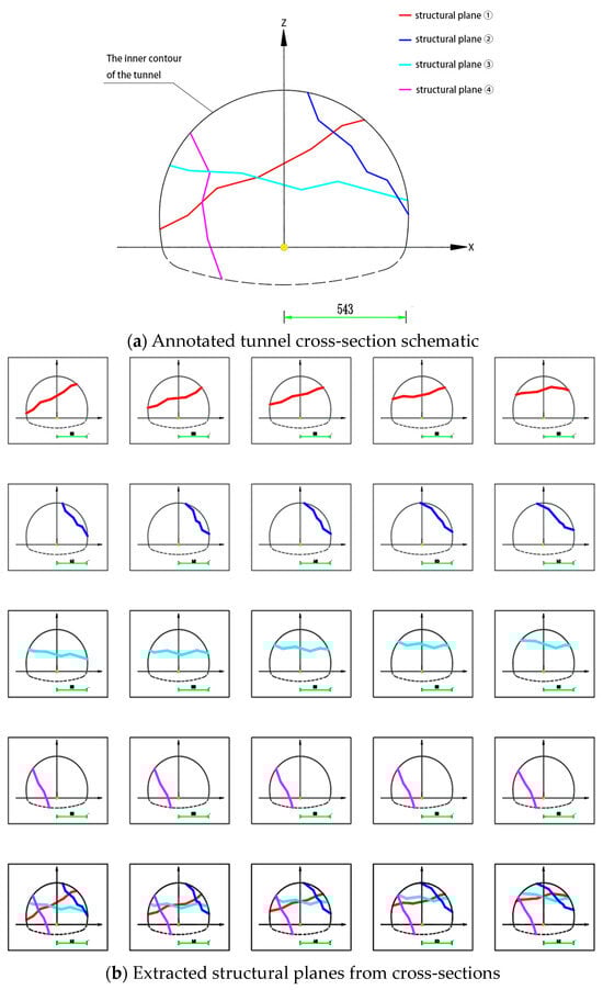
Figure 5. Simulated tunnel cross-section diagram.

• A yellow marker representing the coordinate origin;
• A green segment indicating the X-axis direction, with known physical length;
• Structural planes displayed in distinct RGB values for easy identification.

Using Python and the OpenCV library, the coordinate origin is automatically detected based on its yellow color, and the physical-to-pixel ratio is calculated from the known length of the green segment. This conversion factor is then used to map pixel coordinates into real-world spatial coordinates.

According to the structural layout, two horizontal structural planes (Plane ① and Plane ③) and two vertical ones (Plane ② and Plane ④) were selected for this study. Their boundaries were identified and extracted, as shown in Figure 5b.

3.3. Coordinate Sampling and Transformation

The PNG files were parsed using a custom Python script to extract the pixel coordinates of structural lines. Based on a predefined number of sampling points, the line was evenly segmented, and the endpoints of each segment were used as discrete sampling points.

Since the coordinates extracted from the image are in pixels, they must be converted into physical spatial coordinates using the following formulas:

X_real = X_pixel × R_X

(1)

Z_real = Z_pixel × R_Z

(2)

where X_real and Z_real are the actual physical coordinates, X_pixe and Z_pixel are the coordinates in pixel units, and R_X and R_Z are the conversion ratios in the X and Z directions, respectively.

In this study, the image scale was kept consistent in both directions, so Rx = Rz. To assess the accuracy of pixel-to-physical coordinate conversion, we compared several manually annotated reference points with their transformed spatial coordinates. The mean absolute error between measured and converted coordinates was 1.87 cm, confirming the reliability of the transformation approach. Examples of the sampling result with 10 points on a structural plane curve are shown in Figure 6. All sampled coordinates were stored in .txt files to ensure reproducibility and support further processing.

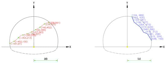
Figure 6. Sampling results of structural lines.

Uniform distribution of sampling points is essential for maintaining interpolation accuracy and computational stability. An automated uniform sampling strategy was implemented in this study, which calculates segment length based on the total curve length and the desired number of sampling points. The program then samples evenly from the start to the end of the curve. Figure 7 presents the sampling results with 20, 50, and 80 points, confirming that the approach ensures evenly distributed points for accurate geometric reconstruction.

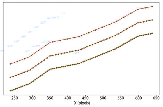
Figure 7. Uniform sampling results with different point numbers.

4. Three-Dimensional Modeling of Structural Planes Based on B-Spline Interpolation

4.1. Overview of the B-Spline Interpolation Method

The B-spline interpolation method, based on piecewise polynomials, enables the construction of smooth and continuous surfaces. It maintains local control over curve segments while avoiding the oscillations that may occur with high-order polynomial interpolation. A B-spline surface is an extension of B-spline functions in both the X and Y parametric directions, and is mathematically expressed as

$$S\left(x,y\right)={\displaystyle \sum _{i=0}^m{\displaystyle \sum _{j=0}^n{N}_{i,k}}}\left(x\right)N_{j,l}\left(y\right)P_{ij}$$

(3)

where S(x,y) is the interpolated surface, P_ij represents the control point matrix, and N_i,k(x) and N_j,l(y) are the B-spline basis functions in the X and Y directions, respectively, with orders k and l.

This study employs B-spline interpolation in three stages: (1) curve fitting from sampled points, (2) construction of a control point grid, and (3) surface interpolation computation.

4.2. Curve Fitting

Because the raw structural data consists of discrete sampling points, curve fitting is first required to generate continuous and smooth lines. Several alternative interpolation methods—such as triangulated irregular networks (TINs), radial basis functions (RBFs), and Kriging—were considered. However, these approaches either lacked sufficient smoothness (e.g., TINs), incurred high computational costs (e.g., Kriging), or offered limited local control (e.g., RBFs).

B-spline interpolation was selected for its favorable balance between computational efficiency, geometric continuity, and local controllability, making it particularly well-suited for modeling irregular yet continuous geological surfaces. In this study, cubic spline interpolation is employed to fit the sampled points, using segmented third-order polynomials that ensure continuity in function value, first derivative, and second derivative across data points. The general mathematical formulation is as follows:

$$S(x)=a_i+b_i(x-x_i)+c_i{(x-x_i)}^2+d_i{(x-x_i)}^3$$

(4)

where x_i are the data points, and a_i, b_i, c_i, and d_i are coefficients determined by interpolation and smoothness constraints.

The implementation was carried out in Python using the CubicSpline function from the SciPy library. The process includes: (1) reading coordinate data from stored files, (2) performing spline interpolation to construct smooth curves, and (3) visualizing the result with Matplotlib.

The interpolated curves of different stations for structural plane ① were plotted in a 3D coordinate system, and the same process was repeated for other structural planes. An example is shown in Figure 8.

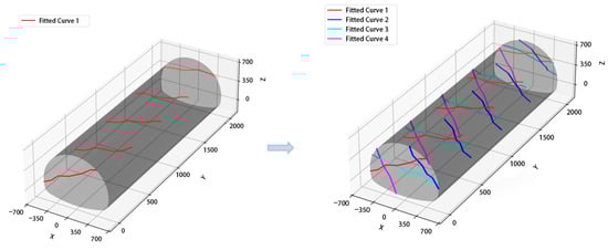
Figure 8. Fitted curves from sampled structural lines.

To evaluate interpolation quality, the mean squared error (MSE) was used:

$$MSE={\displaystyle \frac{1}{n}}{{\displaystyle \sum _{i=1}^n(y_{\mathrm{true}}-y_{\mathrm{pred}},i)}}^2$$

(5)

where n is the number of points, and y_true and y_pred are the actual and predicted Y-values.

The threshold of 75 sampling points was determined through an empirical analysis aimed at balancing model complexity and reconstruction accuracy. As illustrated in Figure 9, the mean squared error (MSE) decreased notably with increasing point density and tended to stabilize beyond 75 points. This threshold thus represents a practical trade-off between interpolation precision and computational efficiency. The fitting results are compared to the original data in Figure 10, demonstrating excellent agreement.

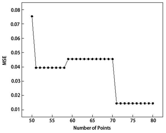
Figure 9. Relationship between MSE and number of sampled points.

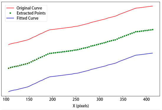
Figure 10. Comparison between fitted and actual curves.

4.3. Control Point Grid Construction

To perform B-spline surface interpolation, control points must be organized into a 2D matrix:

$$P=\{\left.P_{\mathrm{ij}}\right|i=0,1,\dots n;j=0,1,\dots m\}$$

(6)

where iii is the index in the excavation (Y) direction and jjj is the index along the curve (X direction). Each P_ij represents a 3D coordinate. Every interpolated curve at a specific station contributes a row to the control point matrix, forming a complete input grid for surface construction. Figure 11 visually illustrates the distribution of control points used to generate B-spline surfaces.

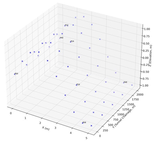
Figure 11. Spatial distribution of control points extracted from multiple tunnel faces for B-spline surface construction.

4.4. B-Spline Surface Calculation

The core of B-spline surface generation lies in the computation of basis functions and surface interpolation using the control point grid. This study used Python’s SciPy library and the bisplrep function to generate the B-spline model tck with degree kx = ky = 3:

$$tck=\mathrm{bisplrep}(X,Y,Z,k_x=3,ky=3)$$

(7)

Here, tck includes knot vectors and weight parameters for surface interpolation. Using the bisplev function, the surface height Z over a mesh grid is evaluated:

$$Z_{grid}=\mathrm{bisplev}(X_{grid},Y_{grid},tck)$$

(8)

The grid was generated using numpy.meshgrid(). Structural plane ① was interpolated at y = 0, 500, 1000, 1500, 2000; y = 0, 500, 1000, 1500, 2000; and y = 0, 500, 1000, 1500, 2000 to visualize the surface sections. The resulting surface Z_grid was visualized using Matplotlib, as shown in Figure 12.

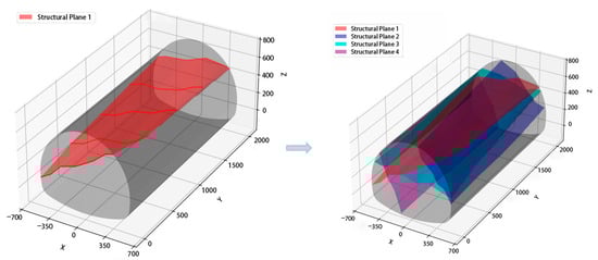
Figure 12. Three-dimensional modeling results of the structural plane.

The smoothness and local control of a B-spline surface are influenced by the spline order k:

k = 2 (quadratic): Ensures C¹ continuity; some sharp transitions may appear.

k = 3 (cubic): Provides C² continuity; balances smoothness and control, suitable for geological surfaces.

k ≥ 4k: Higher continuity (C³ or above), but prone to overfitting and deviation from actual geological morphology.

Although higher-order splines (e.g., k ≥ 4) offer improved continuity, they are more prone to oscillations and overfitting, especially in noisy or irregular data. In our preliminary tests, the cubic spline (k = 3) provided smoother and more geologically plausible surfaces. Therefore, we selected cubic B-splines as a balance between continuity and robustness.

4.5. Surface Visualization

To enhance the visualization of the reconstructed structural surfaces, the study applied several rendering techniques, including gradient color mapping, mesh grid overlay, and light optimization. These techniques improved the visibility of local variations and surface curvature, allowing for full 3D rotation and detailed observation of surface features. As shown in Figure 13, the surface reconstructed for structural plane ① exhibits continuous, smooth transitions across sections without abrupt changes or discontinuities.

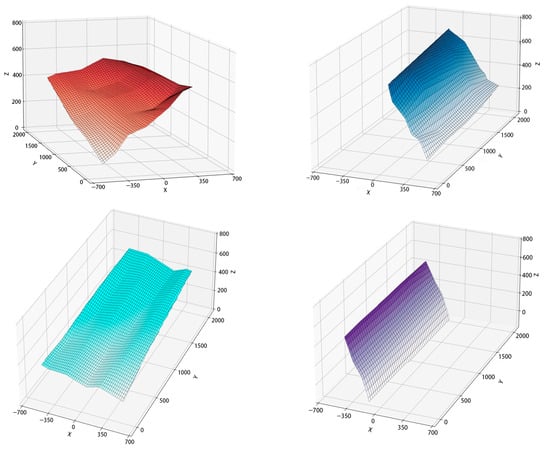
Figure 13. Enhanced visualization of 3D reconstruction results.

5. Engineering Case Study

5.1. Project Background

The Paiyashan Tunnel is a key control project of the Pengba Expressway in Shenzhen, China. Located in the Dapeng New District, it forms an integral part of Shenzhen’s “three-horizontal, three-vertical” expressway network. The tunnel is designed as a dual-bore, four-lane configuration, with a total length of 3445 m for the left bore and 3465 m for the right bore.

Due to the influence of the terrain and connection alignment, the tunnel entrance exhibits significant lateral pressure bias, with the tunnel axis forming an angle of only 35° with the contour lines. The entrance section adopts an extended single-pressure portal with a retaining wall and arch cover, constructed using the cut-and-cover method. This approach ensures construction safety, minimizes excavation volume, and reduces environmental impact. The tunnel exit features a bamboo-cut portal structure. The tunnel alignment passes through geologically complex areas, where the surrounding rock consists primarily of moderately to slightly weathered blocky formations at considerable burial depth, posing high demands for safe excavation.

5.2. Application to Paiyashan Tunnel

To validate the proposed method, images of the tunnel face were collected from station YK3 + 229 to YK3 + 237 at the entrance of the right tunnel. All tunnel face images were captured using the same device (Nikon D750 DSLR, manufactured by Nikon Corporation, Tokyo, Japan; purchased via Taobao, China) at a fixed resolution of 6016 × 4016 pixels. Illumination was provided by portable LED panels, and the camera-to-face distance was maintained at approximately 2.5 m to ensure geometric consistency. As shown in Figure 14, structural plane traces were extracted from the tunnel face images for 3D reconstruction.

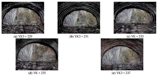
Figure 14. Excavation face views at different mileage stations of the Paiyashan Tunnel.

The detection of structural planes was performed using the YOLOv5 model, which accurately located the target areas. These regions were then processed with the DeepLabV3+ model to conduct pixel-level semantic segmentation and extract precise structural features. Using OpenCV image processing techniques, the centerlines of the structural planes were extracted and plotted within a defined coordinate system (Figure 15). The extracted coordinates were then used to fit curves in 3D space (Figure 16), followed by B-spline interpolation and 3D visualization to obtain the final surface model of the structural plane (Figure 17).

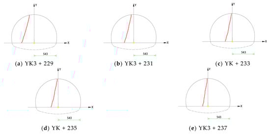
Figure 15. Extraction of structural surface morphology at various chainage points.

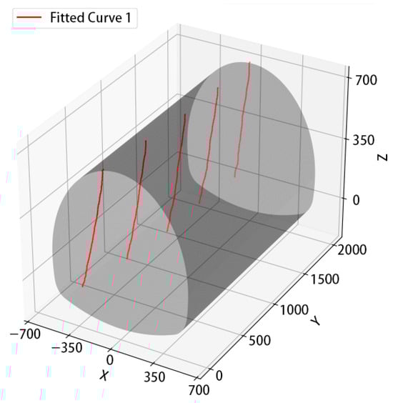
Figure 16. Fitting curve.

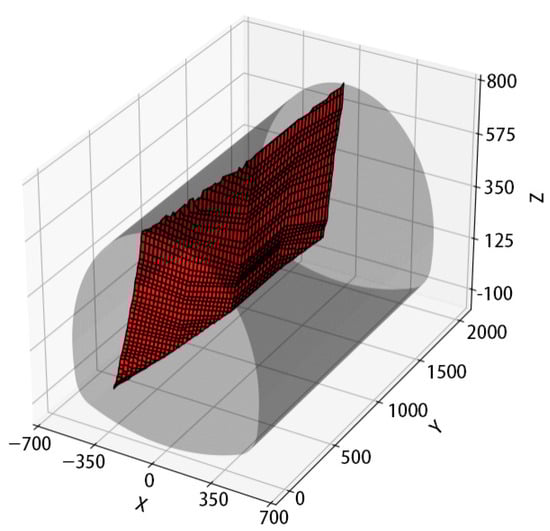
Figure 17. Visualization effect of the structural plane.

5.3. Evaluation of Application Effectiveness

In this study, the Y-coordinate of the station YK3 + 229 was set to 0, while YK3 + 233 was assigned a value of 400, and so on in equal intervals. To evaluate the interpolation accuracy of the reconstructed structural surface, cross-sectional slices were generated at Y = 300 and Y = 700, corresponding to intermediate locations between the actual tunnel stations YK3 + 232 and YK3 + 236. These interpolated cross-sections in the X-Z plane were compared to manually collected feature point data from the corresponding stations. As illustrated in Figure 18, solid lines represent the interpolated sections at Y = 300 and Y = 700, while the scatter points denote the actual measured feature points.

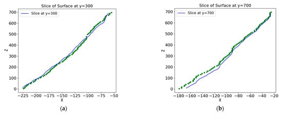
Figure 18. Cross-sectional comparison between observed structural points and the fitted surface at a given chainage. (a) Comparison of interpolated curve and measured data at Y = 300; (b) Comparison of interpolated curve and measured data at Y = 700.

To quantify the surface fitting accuracy, the mean relative error (MRE) was used, calculated as follows:

$$MRE={\displaystyle \frac{1}{n}}{\displaystyle \sum _{i=1}^n\frac{\left|z_{\mathrm{pred},i}-z_{\mathrm{true},i}\right|}{\left|z_{\mathrm{true},i}\right|}}$$

(9)

where n is the number of sample points, and Z_pred,i and Z_true,i represent the predicted and actual elevation values at the iii-th point, respectively.

The MRE values calculated by the Python-based analysis were 0.0234 and 0.0226 for the respective sections, demonstrating that the reconstructed surfaces closely match the actual geological data and validating the reliability of the proposed modeling approach.

The root mean squared error (RMSE) was calculated to quantify the average deviation between the predicted and true elevation values of the reconstructed surface. It is defined as

$$\mathrm{RMSE}=\sqrt{{\displaystyle \frac{1}{n}}{\displaystyle \sum _{i=1}^n{(Z_{\mathrm{pred},i}-Z_{\mathrm{true},i})}^2}}$$

(10)

In this study, the calculated RMSE was 3.12 mm, indicating a high level of surface fitting accuracy.

The Hausdorff Distance (HD) was also employed to evaluate the maximum geometric deviation between the reconstructed and ground-truth point sets. It is defined as

$$\mathrm{HD}(P,Q)=\max \left\{\underset{p\in P}{\sup }\underset{q\in Q}{\inf }\Vert p-q\Vert ,\underset{q\in Q}{\sup }\underset{p\in P}{\inf }\Vert q-p\Vert \right\}$$

(11)

where P and Q represent the sets of predicted and actual 3D points on the structural surface.

The resulting Hausdorff Distance in our test case was 8.57 mm, which further confirms the spatial consistency of the fitted surface.

6. Discussion

Although the proposed method has shown promising potential for accurately and efficiently modeling structural planes in tunnel engineering, some limitations and avenues for further improvement remain. Firstly, the accuracy and robustness of the approach can be influenced by challenging underground conditions, such as low lighting, humidity, dust, severe occlusion, or motion blur, which may affect image quality and subsequent feature recognition. Secondly, despite the inherent adaptability of the B-spline interpolation to arbitrary tunnel profiles—including elliptical, polygonal, or irregular shapes—it inherently relies on sufficient and uniformly distributed input data. Thus, in scenarios where cross-sectional data are partially incomplete or missing, the reconstructed surface essentially represents an extrapolation based on adjacent available sections. As a consequence, unique geological features or abrupt discontinuities within missing segments may be overly smoothed or underrepresented.

To address these challenges in future research, we plan to further enhance the robustness of our deep learning-based feature extraction models through more diverse data augmentation and advanced training strategies, specifically targeting realistic underground disturbances. Additionally, adaptive and locally refined interpolation methods or multi-source data fusion strategies will be explored to better capture sharp geological changes and minimize information loss caused by incomplete datasets. Comprehensive field validations across a broader range of geological conditions, tunnel geometries, and data availability scenarios will also be prioritized. These efforts aim to ensure that the proposed workflow becomes more generalizable and reliable for routine practical applications, potentially complementing or even partially replacing traditional geological survey methods in underground engineering.

7. Conclusions

This study proposes an integrated method for the three-dimensional modeling of structural planes in tunnel surrounding rock, combining deep learning with surface interpolation techniques. A complete workflow—from image recognition and geometric extraction to 3D reconstruction—was developed to address the limitations of traditional methods in terms of efficiency and modeling accuracy. The main conclusions are as follows:

(1)

A deep learning-based structural plane recognition method was developed. By integrating YOLOv5 for rapid object detection and DeepLabV3+ for precise semantic segmentation, the method enables accurate localization and boundary extraction of structural planes. Morphological skeletonization was applied to extract the centerlines, providing a clear and continuous geometric basis for subsequent modeling.

(2)

A geometric mapping model from image to spatial coordinates was established. Using color feature recognition and scale factor conversion, the extracted centerlines were converted into 3D spatial coordinates with physical significance. This ensured spatial consistency and improved modeling accuracy.

(3)

A B-spline interpolation-based method for 3D surface reconstruction was constructed. By fitting structural plane curves across multiple tunnel stations and building a two-dimensional control point network, smooth and continuous 3D surfaces were generated, meeting the modeling requirements in complex geological conditions.

(4)

The proposed method was validated in a real-world engineering project. Taking the Paiyashan Tunnel as a case study, multiple structural planes were successfully reconstructed in three dimensions. The modeling accuracy was quantitatively verified using multiple error metrics, including MRE, RMSE, and Hausdorff Distance, confirming both global and local fitting performance.

In summary, the proposed approach offers an intelligent, efficient, and accurate solution for the identification and 3D reconstruction of tunnel structural planes, with promising potential for application in geotechnical engineering and underground construction projects.

References

- Menendez, E.; Victores, J.G.; Montero, R.; Martínez, S.; Balaguer, C. Tunnel structural inspection and assessment using an autonomous robotic system. Autom. Constr. 2018, 87, 117–126. [Google Scholar] [CrossRef]
- Wang, Q.; Wang, Y.; Jiang, B.; Gao, H.; Ma, F.; Zhai, D.; Cai, S. Testing method of rock structural plane using digital drilling. J. Rock Mech. Geotech. Eng. 2024, 16, 2563–2578. [Google Scholar] [CrossRef]
- Li, Y.; Yuan, L.; Zhang, Q. Brittle rock mass failure in deep tunnels: The role of infilled structural plane with varying dip angles. Int. J. Rock Mech. Min. Sci. 2024, 176, 105721. [Google Scholar] [CrossRef]
- Li, P.; Chen, T.; Liu, Y.; Cai, M.; Sun, L.; Wang, P.; Wang, Y.; Zhang, X. Automatic Identification of Rock Discontinuity Sets by a Fuzzy C-Means Clustering Method Based on Artificial Bee Colony Algorithm. Appl. Sci. 2025, 15, 1497. [Google Scholar] [CrossRef]
- Meng, H.; Mei, G.; Qi, X.; Xu, N.; Peng, J. Deep generative model-based generation method of stochastic structural planes of rock masses in tunnels. Geol. J. 2024, 59, 2566–2583. [Google Scholar] [CrossRef]
- Hendrawan, R.N.; Irsyad, M.; Gunawan, A.; Zainuddin, A.D.; Widiatama, A.J. Study of the Digital Geological Compass in Increasing the Effectiveness and Efficiency of Measuring Geological Structure Data in the Field. J. Geocelebes 2024, 8, 142–150. [Google Scholar] [CrossRef]
- Mehrishal, S.; Kim, J.; Song, J.-J.; Sainoki, A. A semi-automatic approach for joint orientation recognition using 3D trace network analysis. Eng. Geol. 2024, 332, 107462. [Google Scholar] [CrossRef]
- Li, M.; Xiu, Z.; Han, J.; Meng, F.; Wang, F.; Ji, H. Characterization and Stability Analysis of Rock Mass Discontinuities in Layered Slopes: A Case Study from Fushun West Open-Pit Mine. Appl. Sci. 2024, 14, 11330. [Google Scholar] [CrossRef]
- Wang, G.; Yuan, W.; Jiang, F.; Jiang, Y.; Xiao, Z. An approach to rapidly obtaining rock mass structure data during highway tunnel construction and its application. Rock Mech. Rock Eng. 2025, 58, 2243–2272. [Google Scholar] [CrossRef]
- Zhao, Y.; Li, A.; Du, Z.; Chen, Y.; Sun, H.; Zhi, Z. Joint structure detection and multi-scale clustering filtering for tunnel lining extraction from point clouds. IEEE Trans. Intell. Transp. Syst. 2024, 25, 11214–11226. [Google Scholar] [CrossRef]
- Lin, W.; Sheil, B.; Zhang, P.; Zhou, B.; Wang, C.; Xie, X. Seg2Tunnel: A hierarchical point cloud dataset and benchmarks for segmentation of segmental tunnel linings. Tunn. Undergr. Space Technol. 2024, 147, 105735. [Google Scholar] [CrossRef]
- Liu, H.; Li, W.; Zha, H. Classification method of surrounding rock of Highway tunnels based on deep learning technology. Chin. J. Geotech. Eng. 2018, 40, 1809–1817. [Google Scholar]
- Zhao, L.; Hao, S.; Song, Z. Context-aware semantic segmentation network for tunnel face feature identification. Autom. Constr. 2024, 165, 105560. [Google Scholar] [CrossRef]
- Peng, X.; Wang, M. Deep learning-based point cloud semantic segmentation for tunnel face excavation areas in drilling and blasting tunnels. Tunn. Undergr. Space Technol. 2025, 162, 106605. [Google Scholar] [CrossRef]
- Qian, J.; Xue, F.; Wang, T.; Lin, Z.; Cai, M.; Shou, F. Combining SfM and deep learning to construct 3D point cloud models of shield tunnels and Realize spatial localization of water leakages. Measurement 2025, 250, 117114. [Google Scholar] [CrossRef]
- Tan, D.; Tao, Y.; Ji, B.; Gan, Q.; Guo, T. Full-Section Deformation Monitoring of High-Altitude Fault Tunnels Based on Three-Dimensional Laser Scanning Technology. Sensors 2024, 24, 2499. [Google Scholar] [CrossRef]
- Kang, J.; Li, M.; Mao, S.; Fan, Y.; Wu, Z.; Li, B. A coal mine tunnel deformation detection method using point cloud data. Sensors 2024, 24, 2299. [Google Scholar] [CrossRef]
- Zhao, C.; Li, L.; Yin, H.; Zhao, G.; Wang, W.; Huang, J.; Fan, Q. Formal Quantification of Spatially Differential Characteristics of PSI-Derived Vertical Surface Deformation Using Regular Triangle Network: A Case Study of Shixi in the Northwest Xuzhou Coalfield. Remote Sens. 2025, 17, 1388. [Google Scholar] [CrossRef]
- Li, D.; Cheng, B.; Xiang, S. Direct cubic B-spline interpolation: A fuzzy interpolating method for weightless, robust and accurate DVC computation. Opt. Lasers Eng. 2024, 172, 107886. [Google Scholar] [CrossRef]
- Hu, M.; Shi, X.; Wang, T.; Liu, F. A note on cubic polynomial interpolation. Comput. Math. Appl. 2008, 56, 1358–1363. [Google Scholar] [CrossRef]
- Jung, H.B.; Kim, K. A New Parameterisation Method for NURBS Surface Interpolation. Int. J. Adv. Manuf. Technol. 2000, 16, 784–790. [Google Scholar] [CrossRef]
- Shewchuk, J.R. Delaunay refinement algorithms for triangular mesh generation. Comput. Geom. 2002, 22, 21–74. [Google Scholar] [CrossRef]
- Belhachmi, A.; Benabbou, A.; Mourrain, B. A spline-based regularized method for the reconstruction of complex geological models. Math. Geosci. 2025, 57, 89–114. [Google Scholar] [CrossRef]
- Peng, Z.; Sheng, J.; Ye, Z.; Yuan, Q.; Fan, X. A B-spline material point method for deformation failure mechanism of soft–hard interbedded rock. Geomech. Geophys. Geo-Energy Geo-Resour. 2024, 10, 143. [Google Scholar] [CrossRef]
- Duan, S.; Zhang, M.; Qiu, S.; Xiong, J.; Zhang, H.; Li, C.; Jiang, Q.; Kou, Y. Tunnel lining crack detection model based on improved YOLOv5. Tunn. Undergr. Space Technol. 2024, 147, 105713. [Google Scholar] [CrossRef]
- Pan, Z.; Zhang, X.; Jiang, Y.; Li, B.; Golsanami, N.; Su, H.; Cai, Y. High-precision segmentation and quantification of tunnel lining crack using an improved DeepLabV3+. Undergr. Space 2025, 22, 96–109. [Google Scholar] [CrossRef]
Disclaimer/Publisher’s Note: The statements, opinions and data contained in all publications are solely those of the individual author(s) and contributor(s) and not of MDPI and/or the editor(s). MDPI and/or the editor(s) disclaim responsibility for any injury to people or property resulting from any ideas, methods, instructions or products referred to in the content. |
© 2025 by the authors. Licensee MDPI, Basel, Switzerland. This article is an open access article distributed under the terms and conditions of the Creative Commons Attribution (CC BY) license (https://creativecommons.org/licenses/by/4.0/).