Kinematic Tripod (K3P): A New Kinematic Algorithm for Gait Pattern Generation

Abstract

Insects are good examples of ground locomotion because they can adapt their gait pattern to propel them in any direction, over uneven terrain, in a stable manner. Nevertheless, replicating such locomotion skills to a legged robot is not a straightforward task. Different approaches have been proposed to synthesize the gait patterns for these robots; each approach exhibits different restrictions, advantages, and priorities. For the purpose of this document, we have classified gait pattern generators for multi-legged robots into three categories: precomputed, heuristic, and bio-inspired approaches. Precomputed approaches rely on a set of precalculated motion patterns obtained from geometric and/or kinematic models that are performed repeatedly whenever necessary and that cannot be modified on-the-fly to adapt to the terrain changes. On the other hand, heuristic and bio-inspired approaches offer on-line adaptability, but parameter-tuning and heading control can be difficult. In this document, we present the K3P algorithm, a real-time kinematic gait pattern generator conceived to command a legged robot. In contrast to other approaches, K3P enables the robot to adapt its gait to follow an arbitrary trajectory, at an arbitrary speed, over uneven terrain. No precomputed motions for the legs are required; instead, K3P modifies the motion of all mechanical joints to propel the body of the robot in the desired direction, maintaining a tripod stability at all times. In this paper, all the specific details of the aforementioned algorithm are presented, as well as different simulation results that validate its characteristics.

1. Introduction

Locomotion is the act of moving from place to place. To move forward, legged animals, as do insects, use their limbs in a gait pattern. When considering each leg individually, a cycle of the gait pattern is divided into two phases: swing and support. In the swing phase, the limb rises from the ground and moves in the desired direction of movement; the support phase begins when the limb lands and supports a fraction of the total weight of the animal. During the whole cycle, static and/or dynamic equilibrium conditions must be kept for the gait pattern to be stable.

Static stability is achieved when the projection on the ground of the robot’s center of mass (CoM) falls inside the support polygon, defined as the convex hull of all feet in support phase [1,2]. Dynamic stability occurs when the zero moment point (ZMP)—the point with respect to which reaction forces at the contacts between the feet and the ground do not produce any moment in the horizontal direction—is maintained inside the support polygon throughout the gait. Gait patterns whose stability is determined by dynamic conditions allow for faster displacements of the robot because the CoM projection can be located outside of the support polygon for short periods of time [3,4]. Therefore, in order to guarantee stable locomotion, gait synthesizing algorithms must coordinate all limbs of the robot to make it move in the desired direction, while satisfying the static or dynamic equilibrium condition. In general, the stable locomotion is achieved by using precomputed gait patterns for given trajectory and terrain conditions, or by using parametric-adjusting of the gait by heuristic or bio-inspired approaches to cope with trajectory and terrain changes.

The algorithm we propose, called K3P for kinematic tripod, is a real-time kinematic gait generator capable of on-the-fly computing of the limb motions of a legged robot in order to move along an unknown arbitrary trajectory on uneven terrain, while maintaining static equilibrium, maximizing horizontal displacement of the feet contact points, and avoiding collisions between two consecutive limbs. In this paper, we describe some related approaches, analyze the performance of K3P in a virtual test scenario, and use torque estimations to measure the viability of the synthesized gait pattern.

2. Related Work

Legged robots perform different gait patterns depending on the desired horizontal speed and stability criteria [5,6,7,8]. Figure 1a shows a simplified view of the robot limb and the two phases of the gait. Complementarily, Figure 1b shows a complete gait cycle for what is known as static fast gait; as it can be observed, a minimum of three limbs (a tripod) support the robot during walking. The ratio of duration of the support phase to the total cycle duration defines the duty factor $\beta$ of a gait cycle [9], Figure 1b displays gait cycle for a duty factor $\beta =0.5$. Medium speed gaits (or ripple gait) allow for two legs on opposite sides of the robot to be in the swing phase. In slow gait (or tetrapod gait), only one limb at a time performs the swing phase while the rest support the robot; therefore, it is the most stable of the three gaits [10]. So, the problem of synthesizing a gait pattern consists of defining the best sequence of movements for all the robot limbs, where each limb features from one [11,12] up to four degrees of freedom [10,13].

Figure 1. The gait cycle of an hexapod robot. (a) Side view of a leg performing a gait cycle: During the swing phase, the end side of the limb describes a curve or a triangular trajectory. Every DoF is marked with a circle; thus, the limb displayed above has 3 DoF. (b) Fast gait diagram: The beginning and end of the lines, marked with a circle, correspond to the landing and lifting of every limb, respectively. Every limb is marked as a combination of (T)op, (B)ottom, (M)iddle, (L)eft, and (R)ight, according to its position. When the surface is flat and every trajectory for the legs is precomputed, this gait sequence is sufficient [10].

For the purpose of this work, we have classified the related works according to the use of precomputed, heuristic, or bio-inspired approaches to generate the gait.

2.1. Precomputed Approaches

In these approaches, closed mathematical models (geometric and/or kinematic) are used to compute, in advance and for each limb, a sequential set of joint configurations that, when performed, will propel the robot body forward during the support phase, while during the swing phase, the limb tip describes a given parametric trajectory to the next support point, using most commonly sine, Bezier, and triangular trajectories [6,14,15,16,17]. During locomotion, these trajectories are repeated in a logical sequence; in some cases, the trajectory during the swing phase can be adapted to increase or decrease the horizontal travel distance and/or clearance of the gait (see Figure 1b). Furthermore, depending on the chosen mathematical model, actions such as jumping, main body orientation and clearance control may be considered [7]. Another option to a mathematical model are Probabilistic Graphical Models (PGMs) that can be trained and sampled to infer a walking gait [18].

A different paradigm consists of a footstep planning before the actual locomotion. For example, the robot ATHLETE, designed at the Jet Propulsion Laboratory (Pasadena, CA, USA), computes in advance the most useful support points across the terrain before performing any movement [19]. This planning implies that the robot must be able to accurately build a model of its surroundings, using exteroceptive sensors such as rangefinders, increasing the complexity and the total computational cost required for the robot’s locomotion. In contrast, other approaches embrace the uncertainty of the terrain, not focusing on planning the position of all support points beforehand, and instead propelling low-dexterity hexapods with a fixed gait and focusing their efforts on correct state estimation under high-uncertainty circumstances [12].

These approaches allow us to obtain a precise estimation of energy consumption during the locomotion through, for example, a two-layer hierarchical cooperative control scheme [20]. A top-level controller determines the forces and torques that every limb should exert on the body of the robot, so that the robot can follow a given trajectory, while low-level controllers independently command every leg of the robot to exert such forces. Because energy consumption may vary depending on the type of surface the robot is walking on, the travel speed can be adapted by performing slow, medium, or fast gaits, depending on the energy consumed by the actuators driving every limb [15]. Another approach to hierarchical control is to use a top-level exteroceptive methodology to observe and evaluate the terrain and command a low-level routine to switch among precomputed gait patterns, with the objective of maximizing the stability of the robot when traversing uneven terrain [21].

2.2. Heuristic Methods

The major drawback of purely mathematical models is the complexity of the model itself; therefore, roboticists turned to heuristics to generate a gait pattern while still using the precomputed trajectories from an external optimization process under energetic criteria or faulty conditions.

In order to use a simpler model during the gait generation, heuristic approaches enclose a biological notion of locomotion learned from analyzing the movement of animals, expressed as simple rules for the movement of legged robots. Heuristics such as genetic algorithms (GA) can help to generate the walk pattern for a virtual legged robot [22,23], where the main criterion for fitness calculation is the stability of the robot while walking in a straight line over a flat surface, within preset borders and stability [2]. The energy efficiency, traveled distance, and deviation of trajectory from the straight line are used as feedback information for the GA [24]. The final result is a set of static gait patterns for the robot, learned without an explicit mathematical model, from which the robot can choose during locomotion.

Also, Finite State Automata (FSA) can be used to generate walking patterns [25] as well as flow charts [6], as these models can encode a sequence of movements for every limb used during locomotion maneuvers. By definition, these approaches are also static, and adaptability to faulty conditions comes at the cost of increasing the complexity of the FSA or the flow chart.

These approaches can also emulate reflexive motions using a reactive control scheme, allowing a legged robot to react to the irregularities of the terrain it is walking on. These reflexes are triggered when a limb or foot collides unexpectedly with the terrain or an obstacle. The collision detection can be performed with a set of touch sensors [14] or by measuring the electric current, forces, and torques consumed by the actuators on every joint [10].

Heuristics allow for blind-walking, i.e., the robot is able to walk through irregular terrain based only on proprioceptive information [26]. Neural networks can be implemented in hardware with miniaturization and energy efficiency as the main objective [27]. The Virtual Model Control [27] is one of the most relevant heuristics in order to obtain a model from experimental data, simulating the same dynamic behavior of complex mechanical systems using much simpler components such as springs, dampers, masses, etc. The resulting model is less complex but accurate enough to compute the forces acting on the robot body [28,29].

2.3. Bio-Inspired Methods

Most bio-inspired approaches for synthetic gait generation are based on central pattern generators (CPGs). CPGs are oscillators that can generate rhythmic patterns from non-rhythmic signals or no inputs at all. When applied to legged locomotion [23,30,31,32], the rhythmic output of CPGs corresponds to the gait pattern, in response to inputs as a gait velocity command and the proprioceptive sensor information from the limbs of the robot; this means that sensory information plays an important role in CPG-based gait generation [33]. The biggest difficulty with regard to CPGs is determining the correct range of values for the input as well as tuning the internal oscillator parameters, so that the output corresponds to the desired movement of the limbs and the transition between different gaits is smoothly performed [34]. Tuning such parameters is usually performed by trial and error, and some authors have even turned to GAs to tune CPGs [35]. Furthermore, in a decentralized scenario, where there are as much CPGs as limbs, an additional higher-level control is required [36]. In recent works, CPGs can generate a dynamic walking pattern, based on the turning radius of the desired trajectory and switch from tripod, ripple, and tetrapod gaits [37].

2.4. Main Features of K3P Algorithm

The K3P algorithm, the approach we propose for generating the walking gait for legged robots, is based on a centralized kinematic planner. This algorithm performs a steadily fast gait cycle while also being able to drive the robot at an arbitrary speed by dynamically adjusting the duty factor $\beta$. Also, K3P blurs the differentiation between slow, medium, and fast walks under static stability conditions. Basically, K3P moves the robot’s limbs in tripod configurations, keeping a support tripod while swinging the second tripod to a new location, according to the actual desired speed and trajectory of the robot’s center of mass.

The main differences between K3P and other approaches are as follows:

• K3P is self-contained and makes it possible for a legged robot to walk at an arbitrary speed along an arbitrary trajectory over uneven terrain, within the physical limitations of the robot.
• K3P does not require any precomputed limb trajectories for straight or turning maneuvers; instead, it computes the limb trajectories in real-time, to make the robot move straight ahead or in a sharp or wide curve, according to the terrain level.
• Since K3P moves the robot’s center of mass from a supporting tripod to the next one, K3P guarantees static equilibrium during the march while controlling the clearance of the robot to ground level.
• The kinematic planner behind K3P also guarantees slip-free locomotion and collision avoidance among limbs.

Despite the mathematical complexity behind K3P, its use is fairly simple: it requires as input the physical dimensions of the robot and some PD controller gains. We must highlight that none of the limb displacements is computed beforehand, as in most of the mathematical or heuristic approaches; instead, K3P can change robot displacement at any moment. K3P takes into account the actual position and velocity of the center of mass of the robot, as well as its target trajectory, in order to compute the best position for landing the swinging legs to place the next supporting tripod. Furthermore, K3P verifies the stability of the gait by measuring how close the projection of the center of mass is to the support polygon’s edges.

In comparison to precomputed approaches, K3P exhibits flexibility by allowing the dynamic adjustment of the gait pattern during execution in accordance with the specified trajectory. For example, it enables modifications to the body clearance over varied terrain. Moreover, while precomputed methods enforce minimal fixed curvature for the robot’s trajectories, K3P overcomes this constraint by adapting the gait pattern to ensure that the instantaneous turning radius of the robot matches the specified trajectory. Unlike many heuristic methods that demonstrate comparable performance, K3P distinguishes itself through its ease of tuning, facilitated by the concrete nature of all its parameters.

3. Robot Description and Nomenclature

In this section, we will describe the radial hexapod robot on which the K3P algorithm was tested, as well as the nomenclature used (see Table 1). Figure 2a shows the structure of the robot, the main body is circular and the six limbs are evenly distributed along its perimeter; with the center of mass (CoM) at the origin of the B reference frame [14,19,29]. Each limb has three DoF as shown in Figure 2b. By convention, all Z axes are coaxial with the rotation’s axis of each joint. With respect to B, the mounting point for the i-th limb is denoted by the $M_i$ reference frame. The first joint provides the protraction and retraction movements, marked by the variable ${\theta }_s$ in the S reference frame. The L reference frame is located in the second DoF, denoted as ${\theta }_L$; it provides the depression and elevation movements. The third DoF is marked as ${\theta }_k$ in the K reference frame, providing flexion and extension movements. The length of every link are $l_c$, $l_f$, and $l_t$ for the coxa, femur, and tibia, respectively. The supporting point $SP$ is at the point where the limb makes contact with the ground, supporting the body of the robot.

Table 1. Nomenclature.

Parameter	Description
Physical parameters of a limb
${\theta }_s$, ${\theta }_l$, ${\theta }_k$	The three DoF of a limb.
$l_c$, $l_f$, $l_t$	Length of the coxa, femur, and tibia, respectively.
Physical parameters of the gait
$l_h$	Body clearance.
$l_{max}$	Maximum length of the gait.
$l_g$	Limb clearance.
Gait state variables
$\eta$	Swing tripod is landing, moving, or taking off $\in \{-1,0,1\}$.
$\kappa$	Parity $\in \{-1,1\}$.
$\mathbf{P}$	Support positions for the even and odd limbs.
$\rho$	Instantaneous turning radius.
$\mathbf{Z}$	Touch sensor located at $SP$.
K3P input variables
${\mathbf{v}}_c$	Velocity command vector.
${{}^B\mathbf{X}}_k$	The k-th current position of the legged robot.
${\mathbf{K}}_p$	The proportional gains for the PD controller.
${\mathbf{K}}_d$	The derivative gains for the PD controller.
Thresholds and work ranges
$l_{\rho }$	Turning radius threshold.
${\phi }_L$	Angle threshold for two consecutive limbs.
${\mathit{\theta }}_l$	Range of movement for the swing joint.
${\mathit{\theta }}_k$	Range of movement for the knee joint.

Figure 2. The mechanical description of the radial hexapod tested with K3P. (a) The radial hexapod as tested with the K3P algorithm. (b) A detailed mechanical description for one of the legs of the radial hexapod.

The six limbs are divided into two subsets, three non-contiguous limbs form the odd legs subset, while the rest are grouped in the even legs subset (see Figure 2a). Each subset defines a tripod support structure with its own reference frame, E and O, for the even and odd subsets, respectively. The subset supporting the robot defines the parity of the gait $\kappa$; if $\kappa =1$, even limbs support the robot.

To deal with spatial relationships between two reference frames, say frame b with respect to frame a, we used rigid body transformations in homogeneous coordinates denoted as

$${}_a{}^b\mathbf{A}=\left[\begin{array}{cc}{}_a{}^b\mathbf{R}& {}^b{\mathbf{t}}_a\\ \mathbf{0}& 1\end{array}\right]$$

where ${}_a{}^b\mathbf{R}\in SO(3)$ denotes the rotation matrix of frame b with respect to a and ${}^b{\mathbf{t}}_a$ is the position vector of origin of b, also with respect to a.

From the mounting point of the i-th limb, marked as $M_i$ in Figure 2b, the links and joints of each limb form a kinematic chain. The corresponding Denavit–Hartenberg (DH) parameters [38] are summarized in Table 2. Since all limbs are equal, these parameters are valid for all limbs of the radial hexapod. These parameters allow us to compute the rigid body transformation between link n with respect to $n-1$, ${}_{n-1}{}^n\mathbf{A}$. Finally, the rigid body transformation from frame N with respect to the base link ($n=0$) is given by

$${}_0{}^N\mathbf{A}=\prod _{n=1}^N{}_{n-1}{}^n\mathbf{A}$$

Table 2. Denavit–Hartenberg parameters for every leg.

Kinematic Chain
n	D-H Parameter				Description
	d	$\mathit{\theta }$	$\mathit{a}$	$\mathit{\alpha }$
0	0	0	0	0	The mounting point for the leg $M_i$.
1	0	${\theta }_s$	0	0	The swing DoF.
2	$d_2$	0	$l_c$	$\frac{\pi }{2}$	The length of the coxa
3	$d_4$	${\theta }_l-\frac{\pi }{2}$	$l_f$	0	The lift DoF
4	$d_5$	$-{\theta }_k$	$l_t$	0	The knee DoF, tip of leg ($O_{SP}$)

Therefore, with these relations, we can compute from the six sets of joint parameters ${\theta }_s,{\theta }_L,{\theta }_k$, the position of all six leg tips ${\mathbf{SP}}_{\mathbf{i}}$ with respect to B. Also, the inverse kinematic model can be solved for each leg, so the joint parameters can be obtained from the position of each point ${\mathbf{SP}}_{\mathbf{i}}$. Moreover, thanks to these physical dimensions and parameters, we can predict the maximum extension of the gait $l_{max}$, given a desired body clearance $l_h$ and limb $l_g$ clearance over the floor.

4. The K3P Algorithm

In this section, the K3P algorithm will be described (see Algorithm 1), beginning with the description, the objectives of the algorithm, and finally, a global overview. Subsections A to H will discuss the details of every phase of the algorithm.

The main objective of the K3P algorithm is to drive the CoM along an arbitrary trajectory at an arbitrary speed ${\mathbf{v}}_c$, while the two subsets of limbs perform a cyclic gait pattern, swing–support, to follow the movement of the robot’s CoM and to maintain the static stability criteria. The real-time operation of the K3P algorithm is obtained by an update rate ${\Delta }_t$ at which the position of every limb is computed and updated. At the initial state, the two subsets of legs are landed and supporting the body of the robot. The movement begins with the odd subset starting the swing phase, while the even subset remains in the support phase of the gait cycle and propels the CoM B along the desired trajectory by updating the even tripod configuration according to the given velocity ${\mathbf{v}}_c$. Concurrently, K3P also drives the tripod on the swing phase forward ahead in the direction encoded by ${\mathbf{v}}_c$.

Algorithm 1 K3P

Require:  ${\dot{\mathbf{r}}}_d,{{}^B\mathbf{X}}_k,l_h,l_{max},l_g,{\mathbf{K}}_p,{\mathbf{K}}_d,l_{\rho },l_{\phi },{\mathit{\theta }}_l,{\mathit{\theta }}_k$   1: if $\kappa =1$  then $z_k\leftarrow \mathrm{mean}\left({\left[{}_B{}^E\mathbf{A}{\mathbf{P}}_e\right]}_z\right)$   2:     ${{}_B{}^m\mathbf{A}}_k\leftarrow {}_B{}^O\mathbf{A}$,    ${{}_B{}^f\mathbf{A}}_k\leftarrow {}_B{}^E\mathbf{A}$   3: else $z_k\leftarrow \mathrm{mean}\left({\left[{}_B{}^O\mathbf{A}{\mathbf{P}}_o\right]}_z\right)$   4:     ${{}_B{}^m\mathbf{A}}_k\leftarrow {}_B{}^E\mathbf{A}$,    ${{}_B{}^f\mathbf{A}}_k\leftarrow {}_B{}^O\mathbf{A}$   5: if $\eta =0$  then   6:      ${{}^D\mathbf{X}}_k\leftarrow {{}^B\mathbf{X}}_k+{[\dot{\mathbf{r}}{\Delta }_t,l_h-z_k,0,0,\dot{\psi }{\Delta }_t,v_x,v_y,{\displaystyle \frac{l_h-z_k}{{\Delta }_t}},0,0,\dot{\psi }]}^T$   7: else ${{}^D\mathbf{X}}_k\leftarrow {{}^B\mathbf{X}}_k$   8: ${\mathbf{e}}_k={{}^D\mathbf{X}}_{W,k}-{{}^B\mathbf{X}}_{W,k}$   9: $\mathbf{u}\leftarrow {\mathbf{K}}_p{\mathbf{e}}_k+{\mathbf{K}}_d{\displaystyle \frac{\partial {\mathbf{e}}_k}{\partial t}}$,    ${{}^B\mathbf{X}}_{k+1}={{}^B\mathbf{X}}_k+\mathbf{u}{\Delta }_t$   10: ${{}_W{}^B\mathbf{A}}_k\leftarrow {\rm Y}\left({{}^B\mathbf{X}}_k\right)$,   ${{}_W{}^B\mathbf{A}}_{k+1}\leftarrow {\rm Y}\left({{}^B\mathbf{X}}_{k+1}\right)$,    ${{}^m\mathbf{X}}_{B,k}\leftarrow {{\rm Y}}^{-1}\left({{}_B{}^m\mathbf{A}}_k\right)$   11: ${{}_B{}^f\mathbf{A}}_{k+1}\leftarrow {}_W{}^B{\mathbf{A}}_{k+1}^{-1}{\left\{{}_W{}^B\mathbf{A}{}_B{}^f\mathbf{A}\right\}}_k$   12: $\rho \leftarrow {\displaystyle \frac{\Vert \dot{\mathbf{r}}\Vert }{{\left[\dot{\mathbf{q}}\right]}_{\psi }}}$,    ${\theta }_r\leftarrow {\displaystyle \frac{l_{max}}{2\rho }}$   13: ${{}^L\mathbf{X}}_{B,k}\leftarrow \left\{\begin{array}{c}{\left[\frac{1}{2}{l}_{max},0,l_g,{\mathbf{0}}_{1\times 9}\right]}^T\mathrm{if}\left|\rho \right|\ge l_{\rho }\hfill \\ {\left[\frac{1}{2}{l}_{max}cos{\theta }_r,\mathrm{sign}\left({\theta }_r\right)\frac{1}{2}{l}_{max}sin{\theta }_r,l_g,{\mathbf{0}}_{1\times 9}\right]}^T\hfill \end{array}\right.$   14: ${\mathbf{e}}_{L,k}\leftarrow {{}^L\mathbf{X}}_{B,k}-{{}^m\mathbf{X}}_{B,k}$   15: ${\mathbf{u}}_L\leftarrow {\mathbf{K}}_p{\mathbf{e}}_{L,k}+{\mathbf{K}}_d{\displaystyle \frac{\partial {\mathbf{e}}_{L,k}}{\partial t}}$   16: ${{}^m\mathbf{X}}_{B,k+1}\leftarrow {{}^m\mathbf{X}}_{B,k}+{\mathbf{u}}_L{\Delta }_t$   17: ${\Delta }_z\leftarrow {\left[{{}^m\mathbf{X}}_{B,k+1}\right]}_z-{\left[{{}^m\mathbf{X}}_{B,k}\right]}_z$   18: if $\eta =-1\wedge \mathrm{any}\left({\mathbf{Z}}_i\right)$  then ${\left[{\mathbf{p}}_i\right]}_z\leftarrow {\left[{\mathbf{p}}_i\right]}_z+{\Delta }_z$   19: else if $\eta =-1\wedge \mathrm{all}\left({\mathbf{Z}}_i\right)$ then $\kappa \leftarrow (-1)\kappa$,    $\eta \leftarrow 1$   20: else if $\eta =1$  then $\mathrm{highest}\left({\left[{\mathbf{p}}_m\right]}_z\right)\leftarrow \mathrm{highest}\left({\left[{\mathbf{p}}_m\right]}_z\right)-{\Delta }_z$   21: else if $\eta =1\wedge \mathrm{none}\left({\mathbf{Z}}_i\right)$  then $\eta \leftarrow 0$   22: if $\kappa =1$ then ${{}_B{}^O\mathbf{A}}_{k+1}\leftarrow {\rm Y}\left({{}^m\mathbf{X}}_{B,k+1}\right)$,    ${{}_B{}^E\mathbf{A}}_{k+1}\leftarrow {}_B{}^f\mathbf{A}$   23: else ${{}_B{}^E\mathbf{A}}_{k+1}\leftarrow {\rm Y}\left({{}^m\mathbf{X}}_{B,k+1}\right)$,   ${{}_B{}^O\mathbf{A}}_{k+1}\leftarrow {}_B{}^f\mathbf{A}$,   24: ${\mathsf{\Theta }}_s,{\mathsf{\Theta }}_l,{\mathsf{\Theta }}_k\leftarrow$  Inverse kinematics $\left({{}_B{}^O\mathbf{A}}_{k+1},{{}_B{}^E\mathbf{A}}_{k+1},\mathbf{P}\right)$   25: ${}_f{}^m\mathbf{A}\leftarrow {}_B{}^m\mathbf{A}{{}_B{}^f\mathbf{A}}^{-1}$,    $l_{gait}\leftarrow \Vert {{}^m\mathbf{r}}_f\Vert$   26: ${\mathbf{r}}_i={}_B{}^O\mathbf{A}{\mathbf{p}}_{\{1,3,5\}},{\mathbf{r}}_i={}_B{}^E\mathbf{A}{\mathbf{p}}_{\{2,4,6\}}{\phi }_i=arccos\left({\mathbf{r}}_i•{\mathbf{r}}_{i-1}\right)\forall i\in [1,6]$   27: if $l_{gait}\ge l_{max}\vee$ any $({\phi }_i\le l_{\phi })\vee$ any $({\mathsf{\Theta }}_L\notin {\mathit{\theta }}_L)\vee$ any $({\mathsf{\Theta }}_K\notin {\mathit{\theta }}_K)$ then   28:     $\eta \leftarrow -1$   29: Execute $\left({\mathsf{\Theta }}_s,{\mathsf{\Theta }}_l,{\mathsf{\Theta }}_k\right)$

The act of landing the swing tripod to receive the robot’s weight and to allow the other tripod to take off is called a phase shift of the gait cycle. These phase shifts must be performed in such a way that the projection of the CoM on the ground remains at the interior of the supporting polygon at all times, and the total number of phase shifts along the trajectory is kept at minimum, so the step length is maximum. To decide a phase shift of the gait cycle, the algorithm K3P makes use of three different criteria, named ${\mathrm{K}3\mathrm{P}}_1,{\mathrm{K}3\mathrm{P}}_2,\mathrm{and}{\mathrm{K}3\mathrm{P}}_3$, in order to minimize the number of phase shifts during walking while guaranteeing a static stable gait. These criteria are described in subsection F.

The KP3 algorithm uses different frames to describe the configuration of the hexapod robot and to compute the gait: the main reference frame B attached to the robot’s body and CoM, a frame E to describe the tripod formed by the even subset of limbs, and a frame O to describe the odd subset. While in the support phase, any of the two subsets defines a tripod-supporting structure, standing on the ground, so the support polygon corresponds to a triangle at ground level. All support points $S{P}_i$ are described with respect to either E or O reference frames, depending on whether they belong to the even or odd subset (see Figure 2a). As will be shown later, the actual configuration of the robot can be computed from these frames at any time.

In the following subsections, we will introduce some key aspects that give shape to K3P, starting by describing how the CoM is propelled forward along the desired trajectory, given an arbitrary speed command ${\mathbf{v}}_c$. We will also cover how K3P seamlessly distinguishes the forward and turn maneuvers and how K3P performs the phase shift of the gait cycle using the three aforementioned criteria.

4.1. Gait Cycle

From the odd and even subsets of limbs, the supporting tripod of the gait cycle is determined by the parity $\kappa$ of the gait cycle. If $\kappa =1$, the even subset is fixed to the ground, supporting the body of the robot, while the odd subset is moving over ground level, further ahead of the CoM, in a swing motion; the opposite occurs for $\kappa \ne 1$. For each case, the rigid body transformations at time instant k of the swing ${}_B{}^m\mathbf{A}$ and supporting legs ${}_B{}^f\mathbf{A}$ can be obtained using the position of frames E and O, both with respect to B, using the inverse kinematic models of the limbs (lines 1 and 3 of Algorithm 1).

4.2. Propelling Forward the Body of the Robot

The position and orientation of the robot’s body frame B, as well as their corresponding derivatives, with respect to the world reference frame W, describe the desired trajectory of the robot. This target trajectory can be expressed by the state vector:

$${{}^B\mathbf{X}}_{W,k}={[\mathbf{r},\mathbf{q},\dot{\mathbf{r}},\dot{\mathbf{q}}]}^T$$

where $\mathbf{r}={(x,y,z)}^T$ corresponds to the three-dimensional coordinates of B, while vector $\mathbf{q}={(\theta ,\varphi ,\psi )}^T$ contains the three Euler angles that define the orientation of the robot’s body, both with respect to the world frame W.

K3P works at a fixed rate, so after every time step ${\Delta }_t$, the desired position ${{}^D\mathbf{X}}_{W,k}$ for the CoM of the robot is determined by the commanded velocity vector ${\dot{\mathbf{r}}}_d={(\dot{\mathbf{r}},\dot{\mathbf{q}})}^T$ and the current position of the robot (see line 7 of Algorithm 1). This is only carried out if the robot is moving $\eta =0$, otherwise ${{}^D\mathbf{X}}_{W,k}$ remains the same. The ${\left[\dot{\mathbf{r}}\right]}_z$ component is updated to manage any elevation changes of the terrain. To determine ${\left[\dot{\mathbf{r}}\right]}_z$ with respect to B, the difference between the average height of the leg tips $SP$ of the supporting tripod (see lines 1 and 3 of Algorithm 1), and the commanded clearance height is divided by ${\Delta }_t$.

The spatial difference between ${{}^B\mathbf{X}}_{W,k}$ and ${{}^D\mathbf{X}}_{W,k}$ defines an error metric (line 10 of Algorithm 1), which is fed to a PD controller; the result is a control command $\mathbf{u}$ to propel B in the direction encoded in ${\mathbf{v}}_c$ (line 11 of Algorithm 1). Diagonal matrices ${\mathbf{K}}_p$ and ${\mathbf{K}}_d$ contain the proportional and derivative gains.

4.3. Tripod in Support Phase

Given the desired position of the center of mass ${{}_B\mathbf{X}}_{k+1}$ (line 11 of Algorithm 1) and the current tripod supporting the robot ${{}_f{}^B\mathbf{A}}_k$ (lines 1 and 3 of Algorithm 1), K3P defines the new configuration for the support tripod (line 13 of Algorithm 1) constrained by

$${{}_f{}^W\mathbf{A}}_k={{}_f{}^W\mathbf{A}}_{k+1}.$$

(1)

Such a constrain implies that all limbs corresponding to the support tripod remain fixed to the ground with respect to W. In consequence, the gait generated is slip-free and none of the limbs loses contact with the ground. We can solve for ${{}_f{}^B\mathbf{A}}_{k+1}$:

$$\begin{array}{cc}\hfill {\left\{{}_B{}^W\mathbf{A}{}_f{}^B\mathbf{A}\right\}}_k& ={\left\{{}_B{}^W\mathbf{A}{}_f{}^B\mathbf{A}\right\}}_{k+1}\hfill \\ \hfill {{}_f{}^B\mathbf{A}}_{k+1}& ={{}_B{}^W\mathbf{A}}_{k+1}^{-1}{\left\{{}_B{}^W\mathbf{A}{}_f{}^B\mathbf{A}\right\}}_k\hfill \end{array}$$

where ${{}_B{}^W\mathbf{A}}_k$ and ${{}_B{}^W\mathbf{A}}_{k+1}$ are determined by the present and desired poses of B. From these matrices, the inverse kinematic model for the supporting legs can be solved.

4.4. Tripod in Swing Phase

As described earlier, K3P defines dynamically the desired position for the CoM; thus, K3P also defines dynamically the desired position for the tripod during the swing phase. The target position L for the swing tripod is defined with respect to B based on three different parameters: the maximum gait distance $l_{max}$ (see Figure 3a); the instantaneous turning radius of the hexapod $\rho$; and the swing tripod clearance $l_g$.

Figure 3. The position in the $X{Y}_W$ plane and the orientation $\psi$ of the robot, while traversing the lemniscate on uneven terrain. (a) The theoretical maximum gait for the radial hexapod. (b) The dexterous work envelope of two opposite limbs (represented with dotted lines). (c) The shaded area represents the best trade-off between clearance and longest horizontal travel.

The first parameter $l_{max}$ is determined by the dexterous work envelope of two opposite limbs. Figure 3b displays such a dexterous work envelope when ${\theta }_k\in [0,-\raisebox{1ex}{$3\pi $}\!\left/ \!\raisebox{-1ex}{$4$}\right.]$ and ${\theta }_L\in [-\raisebox{1ex}{$\pi $}\!\left/ \!\raisebox{-1ex}{$4$}\right.,\raisebox{1ex}{$\pi $}\!\left/ \!\raisebox{-1ex}{$2$}\right.]$. The envelope defines the horizontal travel distance that a limb can perform. In order to keep phase shifts at minimum, a good compromise between body clearance $l_h$ and the maximum gait distance $l_{max}$ has to be found. In Figure 3c, we plot the maximum limb extension vs. the clearance; the shaded area represents the range of walk heights for which the K3P algorithm can guarantee a horizontal travel distance of 70% of maximum limb extension. Therefore, K3P considers $l_{max}$ to be equal to the 70% of the theoretical maximum extension of the legged robot (see Figure 3a), with a walking height within the shaded range in Figure 3c.

The second parameter that determines the location of frame L is based on the instantaneous turning radius $\rho$ of the CoM B. Such a turning radius is given by the ratio between the current velocity $\dot{\mathbf{r}}=\Vert \dot{x},\dot{y},\dot{z}\Vert$ and the angular velocity around the $Z_B$ axis ${\left[\dot{\mathbf{q}}\right]}_{\psi }$ (line 12 of Algorithm 1). If $\rho$ is above a given threshold $l_{\rho }$, then L is located straight ahead $\frac{1}{2}{l}_{max}$ meters from B in the direction of $\dot{\mathbf{r}}$ (see Figure 4a); otherwise, it is located over the instantaneous circular trajectory such that the arc length from B to L is equal to $\frac{1}{2}{l}_{max}$ (see Figure 4b). Determining the most suitable position for L based on the magnitude of the instantaneous turning radius $\rho$ is how the algorithm differentiates from straight and turning maneuvers.

Figure 4. The two situations that may occur when driving the subset of legs during the swing phase of the gait. (a) Gait forward, $\rho \ge l_{\rho }$, reference frame E moves towards L, which is located straight ahead from B, along the x axis, $d_{max}$ meters. (b) Turning gait, $\rho <l_{\rho }$. Reference frame L is located $d_{max}$ meters ahead over the momentaneous trajectory around the turning point C.

The third and last parameter $l_g$ represents how high the tripod will be raised during the swing phase. This parameter is expressed as a percentage of clearance $l_h$ and it can be changed dynamically, depending of the roughness of the terrain.

The desired position for the tripod in the swing phase is computed in line 13 of Algorithm 1. Similar to Section 4.2, an error metric ${\mathbf{e}}_{L,k}$ is fed to a PD controller to generate a control command ${\mathbf{u}}_L$ over the subset legs in the swing phase, lines 14 and 15 of Algorithm 1, respectively. Then, the position of the tripod performing the swing phase at time instant $k+1$ can be computed (line 16 of Algorithm 1).

4.5. Joint Reconfiguration

In lines 9 and 16 of Algorithm 1, the new positions of the body body frame B and both tripods O and E are obtained, using PD controllers on their target positions.

After the corresponding location for the tripods in the support and swing phases have been updated to follow the movement of the CoM B, their corresponding state vectors ${{}^B\mathbf{X}}_{W,k+1}$, ${{}^O\mathbf{X}}_{B,k+1}$ and ${{}^E\mathbf{X}}_{B,k+1}$ define the spatial relationships between reference frames W, B, O, and E. From here, it is possible to obtain the positions of each leg tip $S{P}_i$ with respect to the robot’s body and, using the inverse kinematics of the 3 DoF RRR limb (line 24 of Algorithm 1), we can compute the values for all articular joints ${[{\theta }_s,{\theta }_l,{\theta }_k]}_{1,2,\cdots ,6}$ [6].

At this moment, K3P tests the stability of the arrangement at time instant $k+1$ by measuring the Euclidean distance from the projection of B on the support polygon to all edges; in case the minimum distance falls below a predefined threshold $l_{thd}$, K3P will command the robot to come to a halt. This rarely occurs because the phase shift tests ${\mathrm{K}3\mathrm{P}}_{1,2,3}$, which will be introduced in the following section, were designed to guarantee a stable gait.

4.6. Phase Shift

While the robot is walking, a phase shift occurs when the two tripods toggle the phase of the gait they are in. The tripod in the support phase takes off to begin the swing phase and the swing tripod lands to start supporting the main body of the robot. In order to maintain the robot in static equilibrium throughout the walking cycle, the K3P algorithm determines when to shift phases based on three different criteria, named ${\mathrm{K}3\mathrm{P}}_1$, ${\mathrm{K}3\mathrm{P}}_2$, and ${\mathrm{K}3\mathrm{P}}_3$. In particular, K3P1 and K3P2 ensure a collision-free gait pattern.

The first condition ${\mathrm{K}3\mathrm{P}}_1$ ensures that every step is as long as mechanically possible for the robot, before the CoM approaches the border of the support polygon too closely, and the gait becomes unstable. For the tripod in the swing phase, ${\mathrm{K}3\mathrm{P}}_1$ measures the horizontal traveled distance from the starting point to the current position of its origin, if the traveled distance reaches the maximum travel distance $l_{max}$ (see Figure 5a), ${\mathrm{K}3\mathrm{P}}_1$ will trigger a phase shift (line 25 of Algorithm 1).

Figure 5. First two criteria that trigger a phase shift. (a) ${\mathrm{K}3\mathrm{P}}_1$. The linear distance between centroids at start and end positions is limited to $l_{max}$ meters. (b) ${\mathrm{K}3\mathrm{P}}_2$. As the even legs turn counter-clockwise, the angle $\phi$ cannot be smaller than ${\phi }_m$.

The second condition ${\mathrm{K}3\mathrm{P}}_2$ avoids collisions between two consecutive limbs during a turning maneuver (line 26 of Algorithm 1). ${\mathrm{K}3\mathrm{P}}_2$ works by measuring the angle $\phi$, formed by the projections on the $X{Y}_B$ plane of two consecutive position vectors ${}^{SP,i}{\mathbf{t}}_B$. If $\phi$ is smaller than a certain threshold, this criterion triggers a phase shift (see Figure 5b).

Together, the criteria ${\mathrm{K}3\mathrm{P}}_1$ and ${\mathrm{K}3\mathrm{P}}_2$ reduce the number of phase shifts when the robot is walking, allowing it to make big steps while advancing and/or turning; additionally, these criteria are enough to control the robot in open-loop blind-walking if all position controllers driving each joint are accurate enough. That said, K3P incorporates the inherent position information of all limbs as a third criterion, named ${\mathrm{K}3\mathrm{P}}_3$, to make sure they are working properly. ${\mathrm{K}3\mathrm{P}}_3$ tests the stability of the inverse kinematics solution; so all joint angles of every limb ${[{\theta }_s,{\theta }_l,{\theta }_k]}_{1,2,\cdots ,6}$ remain within a certain range of operation, avoiding the proximity to the mechanical limits and singularities that otherwise could lead to an unstable walking pattern.

If any of these criteria are met, then the algorithm K3P commands a shift phase of the gait cycle (line 27 of Algorithm 1). The CoM stops its motion to wait for the subset of legs in the swing cycle to land on the ground and begin the stand phase; while the opposite occurs for the subset of legs in stand phase.

4.7. Uneven Terrain

When a phase shift has been triggered, the tripod in the swing phase has to land. If the surface is uneven, the limbs have to adapt to the elevation changes of the surface. In contrast to the tripod control strategy, where the three legs are commanded simultaneously, during landing, each limb is controlled individually and the three landing events are treated separately. By utilizing interoceptive information, the position of each leg is always known. K3P considers that the swing phase has ended only when all three limbs of the swinging tripod have touched the surface, and therefore, it can begin the support phase of the gait cycle (line 19 of Algorithm 1). To adapt to changes in elevation, K3P must receive information when every $SP$ has touched the surface and updates their height with respect to its corresponding reference frame (E or O). The update process is carried out according to the displacement ${\Delta }_z$ performed by the tripod in swing phase while landing (lines 18 and 20 of Algorithm 1). The displacement update ${\Delta }_z$ for the i-th limb (line 17 of Algorithm 1) is expressed as the difference of the z components of two consecutive state vectors of the moving tripod.

The swing phase ends when all limbs have landed, and at this moment, their positions with respect to B have been adapted to the elevation of the terrain below the robot. In order to perceive ground contact, we consider using inexpensive ToF distance sensors (for example, VL53L0X by ST semiconductor). Eventually, when a tripod restarts its swing phase, the limbs take off, starting from the lowest limb (line 20 of Algorithm 1). The update process ${\Delta }_z$ is applied only to those limbs at the same elevation with respect to B, making the limbs separate from the ground in the opposite order on which they landed and move at unison once all the limbs of the tripod have taken off.

Using this approach, the K3P algorithm does not require prior information about the terrain texture. In the Results section, simulations obtained with predefined values of $l_h$ and $l_g$ are shown. However, it is possible to adapt these parameters during execution based on information obtained, for example, from visual data regarding terrain conditions, allowing a higher-level trajectory planning module to modify these parameters.

However, it is important to highlight the limitations of the algorithm: the gait pattern generator will fail when encountering obstacles of significant height, such as large debris or stairs. Additionally, the terrain must be rigid; hence, viscous terrains cannot be considered either.

4.8. Torque Estimation

To test the mechanical viability of the K3P algorithm driving the hexapod robot, we estimated the torques exerted on the knee K, swing S, and lift L joints, as they represent the electric actuators which exert a torque to drive every limb in the commanded direction. Considering that every limb consists of one or more concentrated masses $m_j$, the way to estimate the torque ${\tau }_{S,i}$ for the any given joint, say $\vartheta$, is

$$\begin{array}{cc}\hfill {\tau }_{\vartheta ,i}& =\sum _{j=1}^J{{}^{CoG,j}\mathbf{t}}_{\vartheta }\times m_j\mathbf{g}\hfill \end{array}$$

(2)

where $\mathbf{g}$ is the gravity vector with respect to W, $m_j$ is the mass for the j-th link, and ${{}^{CoG,j}\mathbf{t}}_{\vartheta }$ is the position vector for the CoM of the j-th link with respect to reference frame $\vartheta$. Table 3 lists the three joints of interest along the CoM coordinates for every concentrated mass $m_j$ that exerts a torque on the j-th joint. Using Equation (2), the torques on the knee, swing, and lift joints were estimated, and the results will be shown when we describe the simulation process.

Table 3. Parameters for torque estimation with respect to listed reference frames.

Torque Variables
$\mathit{J}$	Reference Frame	Link	$\mathrm{CoG}$
1	K, Knee	Tibia	${[\raisebox{1ex}{$1$}\!\left/ \!\raisebox{-1ex}{$2$}\right.l_t,0,0]}^T$
2	L, Lift	Femur	${[\raisebox{1ex}{$1$}\!\left/ \!\raisebox{-1ex}{$2$}\right.l_f,0,0]}^T$
3	S, Swing	Coxa	${[\raisebox{1ex}{$1$}\!\left/ \!\raisebox{-1ex}{$2$}\right.l_c,0,0]}^T$

5. Test Results

In this section, we show the test results of the K3P algorithm when commanding an hexapod robot with a radial base of $0.65$ m in a virtual uneven terrain. The numerical values for all physical dimension and parameters are listen in Table 4. The results shown in this section were obtained from computations on Matlab in order to simulate the kinematics of the robot.

Table 4. Simulation parameters.

Hexapod
${\theta }_l$	$[-\raisebox{1ex}{$2\pi $}\!\left/ \!\raisebox{-1ex}{$9$}\right.,\raisebox{1ex}{$2\pi $}\!\left/ \!\raisebox{-1ex}{$9$}\right.]$	${\theta }_k$	$[-\raisebox{1ex}{$\pi $}\!\left/ \!\raisebox{-1ex}{$4$}\right.,\raisebox{1ex}{$\pi $}\!\left/ \!\raisebox{-1ex}{$4$}\right.]$
$l_{max}$	0.165 m	${\phi }_L$	${15}^{\circ }$
$l_c$	$0.06$ m	$l_f$	$0.16$ m
$l_t$	$0.16$ m	$v_B$	0.15 m/s
${{}^B\mathbf{X}}_{W,0}={[0,0,0.2,0,0,0,0,0,0,0,0,0]}^T$
Controller gains
${\mathbf{K}}_p=diag(2,2,2.5,0,0,0.9,0,0,0,0,0,0)$
${\mathbf{K}}_d=diag(0.05,0.05,0.1,0,0,0.05,0,0,0,0,0,0)$
Lemniscate parameters
a	1.75	b	$1.15$
c	0.0	$ϵ$	30

During the simulation, the speed commands ${\mathbf{v}}_c$ for the robot were generated so that it describes a lemniscate trajectory. We chose the lemniscate trajectory because it defines two turns in opposite directions and two almost straight segments for the robot to travel. The parametric equations of the lemniscate ${\mathbf{r}}_d\left(s\right)$ is shown in Equation (3):

$${\mathbf{r}}_d\left(s\right)=\left[\begin{array}{c}{x}_d\left(s\right)\\ y_d\left(s\right)\\ z_d\left(s\right)\\ {\psi }_d\left(s\right)\end{array}\right]=\left[\begin{array}{c}asin\left(\frac{s}{ϵ}\right)\\ bsin\left(\frac{2s}{ϵ}\right)\\ csin\left(\frac{3s}{ϵ}\right)\\ arctan2({\dot{y}}_d,{\dot{x}}_d)\end{array}\right]$$

(3)

For this numerical example, the robot is commanded to follow a lemniscate covering a rectangular region of $3.5$ m long and $2.3$ m wide; the values for all parameters of the lemniscate equations are listed in Table 4. For a given speed value $v_B$ and time step ${\Delta }_t$, we iteratively computed the increment for the parameter ${\Delta }_s$ that yields an equal incremental displacement ${\Delta }_{{\mathbf{r}}_d}=v_B{\Delta }_t$. This incremental displacement is then used as the input command for the K3P algorithm ${\mathbf{v}}_c$ (Section 4.2) as

$${\mathbf{v}}_c=\left[\begin{array}{c}{v}_x\\ v_y\\ v_z\\ \dot{\psi }\end{array}\right]=\left[\begin{array}{c}{\dot{x}}_d(s+{\Delta }_s)\\ {\dot{y}}_d(s+{\Delta }_s)\\ {\dot{z}}_d(s+{\Delta }_s)\\ arctan2({\dot{y}}_d+{\Delta }_s,{\dot{x}}_d+{\Delta }_s)\end{array}\right]$$

Figure 6a shows how K3P drove the hexapod around the lemniscate trajectory over uneven terrain, as well as the trail of all limbs; the initial state of the robot was

$${{}^B\mathbf{X}}_{W,0}={[0,0,0.16,{\mathbf{0}}_{1\times 9}]}^T$$

Figure 6. K3P driving the hexapod robot over uneven terrain, describing the lemniscate trajectory. (a) Walk gait around the lemniscate over uneven terrain (lighter colors indicate higher elevations of the terrain). (b) Desired ($x_d\left(t\right)$ and $y_d\left(t\right)$) and actual ($x\left(t\right)$ and $y\left(t\right)$) trajectories. (c) The transient $\psi$ response. (d) Walking height $z\left(t\right)$ vs. terrain elevation $z_d\left(t\right)$.

Figure 6b shows the trajectory described by the CoM of the robot, overlapping the desired trajectories in the $X{Y}_W$ plane. Figure 6c shows the transient response at the beginning of the trajectory when the hexapod aligns itself with the lemniscate trajectory from its initial state; the shaded areas represent the moments at which the even subsets of legs are at the swing phase of the gait cycle. The reader can verify that after every phase shift is triggered, the desired angle of orientation ${\psi }_d\left(t\right)$ equals $\psi \left(t\right)$; this causes the robot to stop spinning while the swinging tripod lands. Figure 6d displays how K3P adapts to the elevation of the terrain $z_d\left(t\right)$ as measured from right below B. K3P tries to maintain a constant walking height $z\left(t\right)$ with respect to the surface elevation ≈0.16 m (Section 4.7). 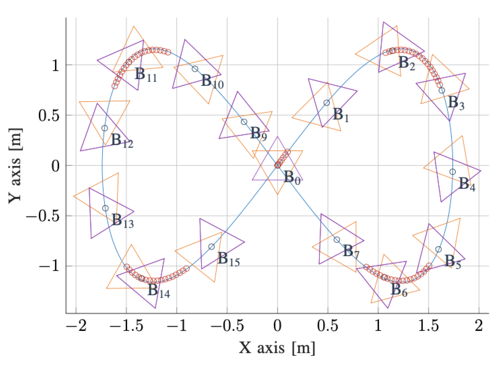Figure 7 shows several footprints of the hexapod right after a phase shift occurs, and both subsets of legs are touching the ground. The corresponding locations of $B_{1,2,\cdots ,15}$ are shown to display that the gait is stable because B is within the support polygon of the vehicle. Furthermore, Figure 7 shows where the turning radius is smaller than the threshold ${\rho }_m=0.8$ m used in the simulation to better determine the desired location L for the swing tripod, as discussed in Section 4.4.

Figure 7. The stability of the walking gait. Consecutive orange dots over the trajectory represent the location of B where $\rho <0.8$ m.

Figure 8a represents the first 40 s of simulation when the hexapod traverses the lemniscate trajectory; the shaded areas show when the even tripod is in the swing phase, while the white areas show where the odd tripod is performing the swing phase of the gait cycle. At every change in shading, the graph shows the criterion triggering the phase shift at the specific moment in time it occurred: number 1 for ${\mathrm{K3P}}_1$, number 2 for ${\mathrm{K3P}}_2$, and 3 for ${\mathrm{K3P}}_3$. At the beginning of the simulation, when the hexapod robot aligns with the lemniscate, ${\mathrm{K}3\mathrm{P}}_2$ triggers the phase shift because the legs were getting too close to each other during the turning maneuver; this corresponds to the transient response in the $\psi$ angle as displayed in Figure 6c. Then, ${\mathrm{K}3\mathrm{P}}_1$ triggers the phase shift because the traveled distance of the swinging tripod is longer than $l_{max}$. The dotted lines correspond to the thresholds $\frac{1}{2}{l}_{max}$ and ${\phi }_m$, for the maximum gait distance and minimum angle between two consecutive legs, respectively. Moreover, to display that K3P is capable of commanding the robot to move at an arbitrary velocity through an arbitrary trajectory, the graph in Figure 8a displays a change in velocity, commanded right after the fourth phase shift at $t\approx 22$ s. The velocity is doubled from $v=0.02$ m/s to $v=0.04$ m/s; the change in velocity can be observed from the duration of the swing phase, where they become narrower after $t\approx 22$ s because it takes less time for the robot to cover the maximum traveled distance $l_{max}$. Note, however, that the change in speed can be commanded at any given time, changing immediately the duty factor $\beta$.

Figure 8. The phase shifts and torques generated when the hexapod robot traverses the lemniscate. Only the first 40 s of simulation are shown. (a) The phase shifts triggered during the first 40 s of the simulation. The commanded speed starts at $v=0.02$ m/s; after the fourth phase shift ($t\approx 22$ s), it was changed to $v=0.04$ m/s. (b) For the odd tripod, the torques exerted on the L and K joints around the z axis.

After running the simulation, we estimated the torques exerted on every joint of the robot. We modeled the robot as a set of discrete masses, listed in Table 5, whereby the overall mass of the robot is approximately 1.6 kg. Figure 8b shows the resulting torques on the knee and lift joints for the odd subset of limbs during the same period of time and phase shifts as previously discussed for Figure 8a. Torques for the even subset of limbs are in the same order of magnitude, since the robot is symmetrical. Because the axis of rotation of the knee and lift joints are coaxial with the two axes [K${]}_z$ and $[L$${]}_z$, in Figure 8b, we only show ${\left[{\mathbf{\tau }}_{L,i}\right]}_z$ and ${\left[{\mathbf{\tau }}_{K,i}\right]}_z$. We omitted the torque exerted on the swing joint, because ${\left[{\mathbf{\tau }}_{S,i}\right]}_z\approx 0$. As it can be observed, the maximum torques exerted on the lift and knee joints occur when the even tripod is in the support phase of the gait cycle; furthermore, the maximum absolute values were 1.36 Nm and 0.60 Nm for the ${\left[{\mathbf{\tau }}_{L,i}\right]}_z$ and ${\left[{\mathbf{\tau }}_{K,i}\right]}_z$ axes, respectively, which are manageable for commercially available servo motors.

Table 5. Discrete masses that form the robot.

Mass Distribution of the Robot
Qty.	Link	Unit Mass [gr]	Subtotal
1	Main body	640	640
6	Coxa	80	480
6	Femur	53	318
6	Tibia	26	156
Total weight			1594

As mentioned in Section 4.4, the K3P algorithm can command the swing tripod to increase or decrease the maximum clearance of the robot. Figure 9 displays two different values of clearance when the robot travels in a straight line uphill: the first (see Figure 9a) with a clearance equal to 50% of $l_h$ and the second with a clearance of 90%. The latter causes the support point $SP$ to travel almost as high as the CoM B. If required, the walk clearance can be updated at any moment to better adapt to the terrain’s changes in elevation. Section 4.4 also shows the profile of every gait cycle that the K3P algorithm describes. Right after a phase shift is triggered, the limbs are taken to land to begin the support phase of the gait cycle.

Figure 9. The trajectories of $S{P}_1$ when K3P drives the hexapod uphill (black solid line) at two different settings for the maximum height. The hexapod robot moves from left to right, the trajectory of B is also shown. For simplicity, we only show the trajectory for leg number 1. (a) The limbs are swinging at 50% of clearance. (b) The limbs are swinging at 90% of clearance.

6. Conclusions

In this article, the K3P algorithm is proposed as a novel approach for dynamic gait generation for hexapod robots. This new algorithm is based on a kinematic planner for the legs organized as tripods. The core of K3P are three shift phase conditions, ${\mathrm{K}3\mathrm{P}}_{1,2,3}$, that ensure the static slip-free stability of the robot throughout its operation, without requiring any precomputed paths or trajectories whatsoever.

The methodology and numerical results are presented for a radial hexapod traversing a lemniscate trajectory, shown as a versatile methodology when commanding an hexapod. Compared to other approaches, K3P does not require any precomputed information from the trajectory to be followed, nor the trajectory for every support point $S{P}_i$, nor precomputed gait patterns. Instead, all trajectories for every tripod were dynamically generated in real-time and made possible that B described a smooth arbitrary trajectory at an arbitrary velocity while the support points remained still over the uneven surface that the robot was walking on. Additionally, K3P is able to dynamically change the clearance of the robot, and we studied the trade-off between clearance vs. step length, given the physical dimensions of the robot.

The K3P algorithm is executable on commercially available embedded computers, using fast linear algebra computation libraries, such as Lapack. Modern CPUs support instruction sets enabling parallelization, such as Single Instruction Multiple Data (SIMD), while GPUs can further enhance the algorithm’s execution speed. The possibility of implementing the algorithm on an FPGA can also be considered. Consequently, K3P algorithm finds application in real-time scenarios for robot control. However, it can also be utilized in offline contexts. For example, K3P could serve as a teaching tool for neural networks, with K3P criteria employed to reinforce the learning process of walking.

Because the K3P algorithm performs at real-time and under static stability, it can change the direction of movement of the robot at any given moment. This can be useful if the robot performs in an ever-changing environment with static and dynamic obstacles, e.g., humans or other mobile robots. Such is the case in collaborative robotics; in this emerging research field, robots perform alongside humans or other robots [25]. K3P can offer a development opportunity in collaborative robotics because it can make the robot stop or perform an immediate change in direction of movement when close to a moving obstacle or in a dangerous situation.

The viability of the algorithm is proven by estimating the torques exerted on the knee and lift joints, which are below the maximum torque of commercially available electric servo motors.

As it was shown in the previous section, the K3P algorithm can drive a hexapod robot over irregular terrain without planning in advance every step of the robot at an arbitrary speed. This key design choice for K3P has an important implication: a higher-level trajectory planner can determine the most suitable path for the robot to follow, so that all traversed portions of the terrain can support a footstep. Therefore, K3P can be described as a low-level kinematic planner for a hexapod robot operating in open loop. Its features would allow us to use it alongside different abstraction models of a hexapod to make the robot change its shape when walking in confined environments [39]. Changing the shape of the robot when walking can be useful to adapt to not only uneven terrain as shown here, but to also adapt to constrained and unstructured environments such as a tunnel.

7. Future Work

As future work, we plan to test K3P with an actual robot. The main purpose will be to integrate this algorithm as a low-level feature, allowing for higher-level algorithms to plan the desired trajectory for the robot. Additionally, we plan to integrate an Inertial Measurement Unit as a loop back sensor to work in a closed-loop scheme for the position and pose of the robot; this would make it possible for the robot to display some level of adaptation to sudden external perturbations (mud, gliding, external agents, etc.).