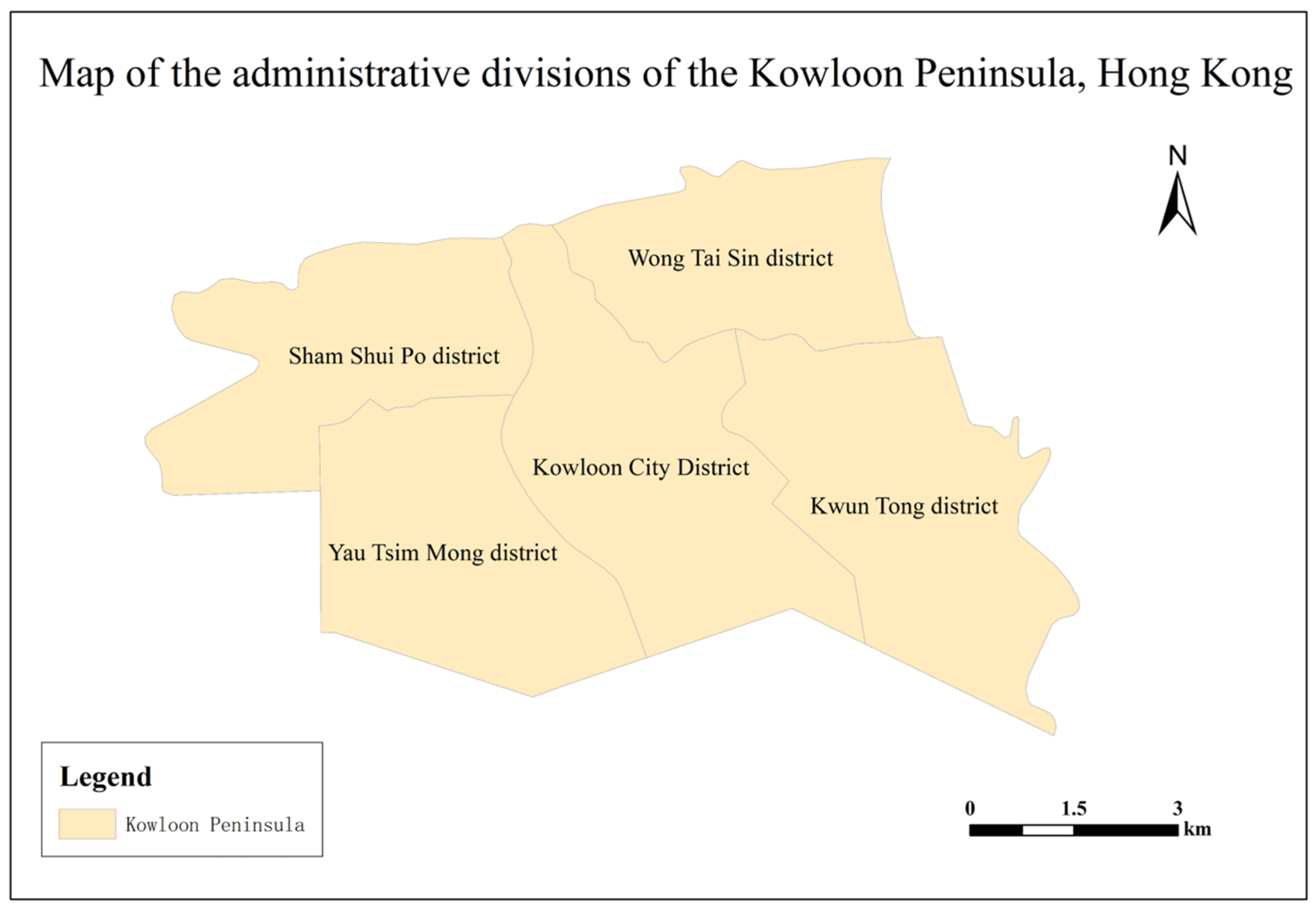
You are currently viewing a new version of our website. To view the old version click .
Applied Sciences
  • Article
  • Open Access

3 March 2024

An Urban Built Environment Analysis Approach for Street View Images Based on Graph Convolutional Neural Networks

,
,
,
,
and
1
School of Information Engineering, Shanxi Vocational University of Engineering Science and Technology, Jinzhong 030606, China
2
School of Computer Sciences, China University of Geosciences, Wuhan 430074, China
3
Hubei Key Laboratory of Intelligent Geo-Information Processing, China University of Geosciences, Wuhan 430074, China
4
Yichang Key Laboratory of Intelligent Vision Based Monitoring for Hydroelectric Engineering, China Three Gorges University, Yichang 443002, China
This article belongs to the Special Issue Emerging GIS Technologies and Their Applications

Abstract

Traditionally, research in the field of traffic safety has predominantly focused on two key areas—the identification of traffic black spots and the analysis of accident causation. However, such research heavily relies on historical accident records obtained from the traffic management department, which often suffer from missing or incomplete information. Moreover, these records typically offer limited insight into the various attributes associated with accidents, thereby posing challenges to comprehensive analyses. Furthermore, the collection and management of such data incur substantial costs. Consequently, there is a pressing need to explore how the features of the urban built environment can effectively facilitate the accurate identification and analysis of traffic black spots, enabling the formulation of effective management strategies to support urban development. In this study, we research the Kowloon Peninsula in Hong Kong, with a specific focus on road intersections as the fundamental unit of our analysis. We propose leveraging street view images as a valuable source of data, enabling us to depict the urban built environment comprehensively. Through the utilization of models such as random forest approaches, we conduct research on traffic black spot identification, attaining an impressive accuracy rate of 87%. To account for the impact of the built environment surrounding adjacent road intersections on traffic black spot identification outcomes, we adopt a node-based approach, treating road intersections as nodes and establishing spatial relationships between them as edges. The features characterizing the built environment at these road intersections serve as node attributes, facilitating the construction of a graph structure representation. By employing a graph-based convolutional neural network, we enhance the traffic black spot identification methodology, resulting in an improved accuracy rate of 90%. Furthermore, based on the distinctive attributes of the urban built environment, we analyze the underlying causes of traffic black spots. Our findings highlight the significant influence of buildings, sky conditions, green spaces, and billboards on the formation of traffic black spots. Remarkably, we observe a clear negative correlation between buildings, sky conditions, and green spaces, while billboards and human presence exhibit a distinct positive correlation.

1. Introduction

With the rapid development of cities, people’s living standards gradually improve; the number of motor vehicles increases; and the problem of the unbalanced development of people, vehicles, and roads becomes more prominent, which can easily produce traffic hazards and lead to traffic accidents [1,2,3]. Traffic black spots are defined as locations with a high incidence of traffic accidents, which account for only 0.25% of the total road network mileage, although the number of traffic accidents occurring in them accounts for 25% of the total number of accidents [4,5,6,7]. Therefore, accurately identifying traffic black spots can reduce the occurrence of traffic accidents.
How to accurately identify traffic black spots on the basis of existing data has not yet been uniformly determined. In previous studies, traffic accident data have mostly come from the historical accident records of the traffic management department, and the number of traffic accidents is analyzed to determine the locations of the traffic black spots by using mathematical and statistical methods [8,9,10]. The data are relatively singular and not easy to collect and manage, and more importantly the number of accident features is small, which does not allow for a specific analysis of the causes of traffic black spots. The emergence of geographic big data and the rapid development of machine learning and deep learning make it possible to portray the built environment of urban roads from street view image data [11,12,13]. In real life, traffic accidents are also more likely to occur on densely populated streets with crowded and dilapidated buildings, without better road infrastructure, and with missing road markings and blurred and uneven road surfaces [14,15,16]. These features are all part of the built environment of urban roads, which can be described by street image data. Using the existing deep learning semantic segmentation technology, street image data can be segmented into more than 100 urban built environment features [13], which could be very useful as a supplement to a traffic management department’s historical accident record data feature factors, so as to carry out a specific analysis of the formation of the traffic black spots.
Traffic black spot identification is the focus of research in the field of traffic safety. By accurately identifying traffic black spots in urban roads, urban traffic management departments can make targeted improvements to reduce the incidence of traffic accidents to protect people’s right to life, property, and health. In this paper, on the basis of the above research, street view image data are assessed using deep learning semantic segmentation technology to describe the characteristics of the built environment of urban roads, so as to obtain the information containing the characteristics of the built environment of urban roads, which can be used to identify black spots in urban road traffic. At the same time, the data from traffic accidents and street view image data are processed and constructed into the structure of a graph network and a graph convolutional neural network (GCNN) model is used to identify black spots in traffic. This GCNN model is used for the recognition of traffic black spots to make the recognition results more accurate. Firstly, taking the road intersection as the research unit, the street view image data are extracted using a semantic segmentation model to portray the built environment of urban road intersections and machine learning models, such as support vector machine (SVM), gradient boosting (GBDT), and random forest (RF) models, which are used to identify the traffic black spots. Then, the traffic black spot recognition method is improved by considering that the interconnection of built environment features of adjacent road intersections will have an impact on the formation of traffic black spots. The traffic accident data and street scene image data are processed, the graph network structure is constructed, and the graph convolutional neural network (GCNN) model is used for the recognition of traffic black spots. In the analysis of the causes of traffic black spots, the importance of each feature of the built environment of urban road intersections on the formation of traffic black spots and the interconnections between each feature are analyzed to make the research results more reliable. The proposed method can effectively improve the urban road planning and design process and make human environment planning and design more scientific, more reasonable, and more in line with the standard of the ideal modern city. In addition, the street scene image data are easier to collect and manage, which can save a significant amount of manpower cost and time cost.
In this paper, we take the Kowloon Peninsula of Hong Kong as the study area and road intersections as the study unit, and traffic black spot identification and cause analysis are the research objectives. The built environment feature dataset of urban road intersections is constructed from street view images by the semantic segmentation model, which is used to identify and analyze the causes of traffic black spots at urban road intersections. The main contributions of this study are as follows:
(1)
By capitalizing on the characteristics of the built environment surrounding urban road intersections, and employing techniques such as random forest modeling, traffic black spots are identified for each individual road intersection;
(2)
To enhance the methodology for detecting traffic black spots, a graph network structure is proffered as a valuable approach. Recognizing the spatial correlation intrinsic to traffic black spots, this research adopts road intersections as nodes and establishes interconnections between adjacent road intersections as edges within the graph. By incorporating the built environment characteristics of the urban setting as node attributes, a graph network topology is constructed. Subsequently, a graph convolutional neural network is employed to carry out traffic black spot identification;
(3)
Starting from the characteristics of the built environment of urban road intersections, we analyze their correlation with the formation of traffic black spots, further expanding the research ideas in this direction.

3. Study Area and Data

3.1. Study Area

The study area selected for this paper is the Kowloon Peninsula of Hong Kong, located in the northern part of the Hong Kong Special Administrative Region, a major administrative region and commercial center of Hong Kong, with a total area of about 46.93 square kilometers, including five districts, namely Yau Tsim Mong, Sham Shui Po, Kowloon City District, Wong Tai Sin, and Kwun Tong, which is one of the three major districts of Hong Kong (Figure 1). With a more developed economic and transportation network, and many famous scenic spots as well as major roads, it is an important convergence of logistics and people flow. As a typical urban area in Hong Kong, the Kowloon Peninsula has a very high traffic density and traffic congestion is very common, especially during the morning and evening peak periods.
Figure 1. Illustration of the administrative divisions of the Kowloon Peninsula of Hong Kong.
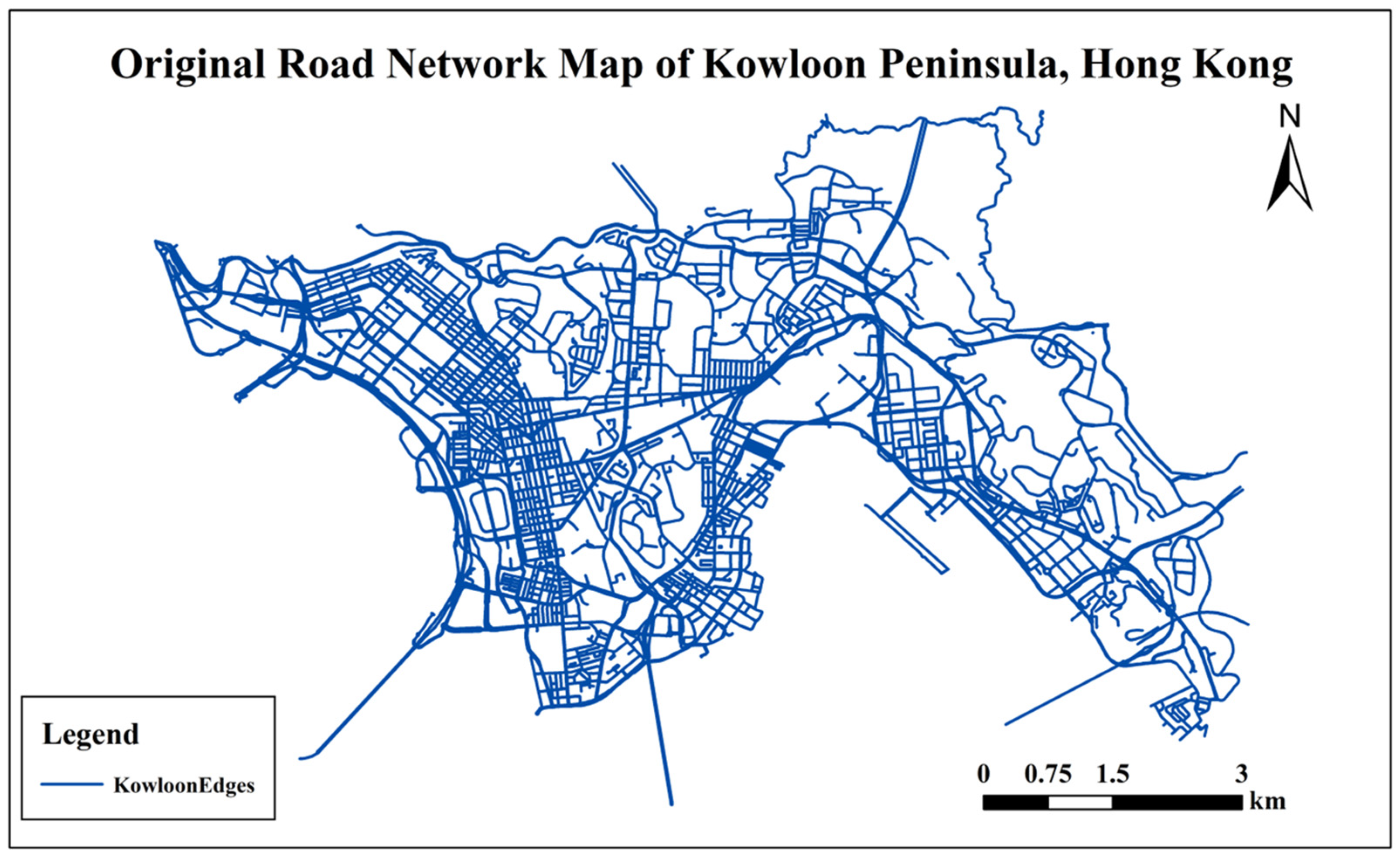
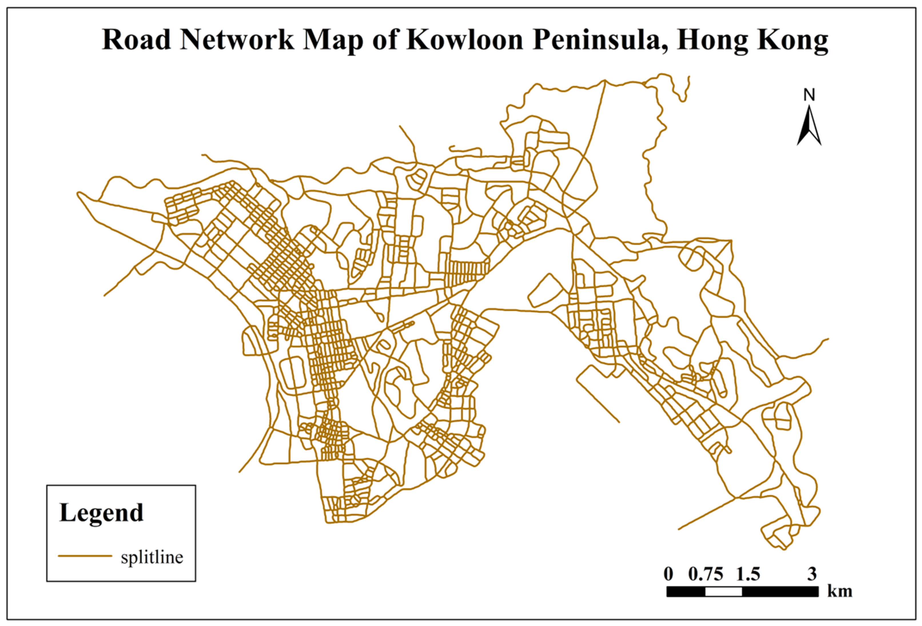
3.2. Research Data Acquisition and Processing

The dataset used in this study is a self-constructed dataset, which consists of three parts:
Road network data: The road network data need to be obtained on the OpenStreetMap (OSM) website by itself, and the original data type obtained is in the OSM format, which needs to be converted into the SHP format and then processed.
Traffic Accident Data: The traffic accident data include a total of 10,392 data points with latitude and longitude coordinates in the Kowloon Peninsula area of Hong Kong for two years in 2014 and 2015, and the distribution is shown in Table 2.
Table 2. Number of traffic accidents distributed in various districts of Kowloon Peninsula.
Street View Image Data: The street view image data were collected using the Tencent Street View platform with Python 3.8 crawler technology, and a total of 8044 street view sampling points were selected and 32,176 street view images were acquired.

3.2.1. Road Data Acquisition and Processing

The road network map of the Kowloon area of Hong Kong obtained from the OpenStreetMap (https://openmaptiles.org/; Access Date: 1 December 2023) website contains geographic information about the roads, streets, highways, bridges, tunnels, sidewalks, and other transportation facilities and buildings in the area. The obtained road network of the Kowloon Peninsula area of Hong Kong is shown in Figure 2.
Figure 2. Road network map of Kowloon Peninsula, Hong Kong.
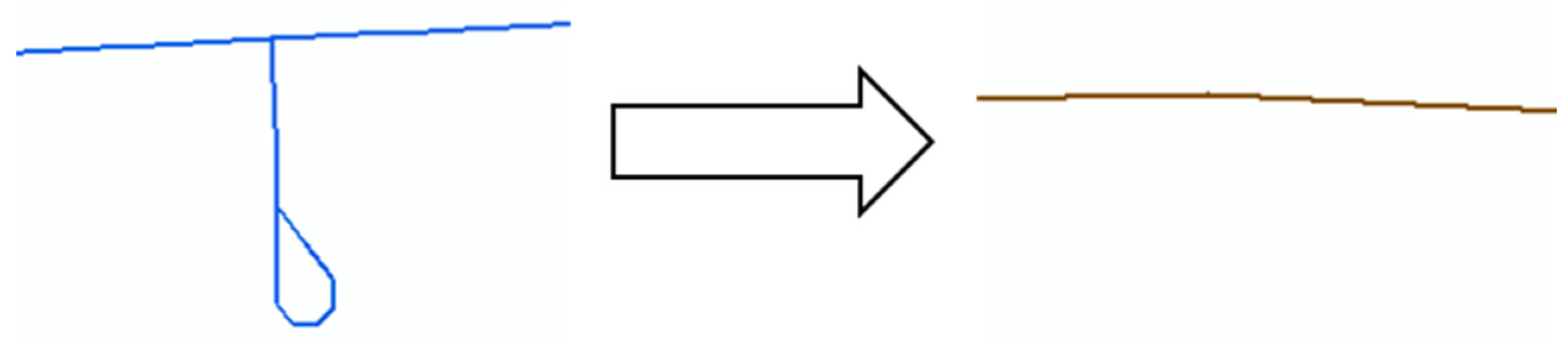
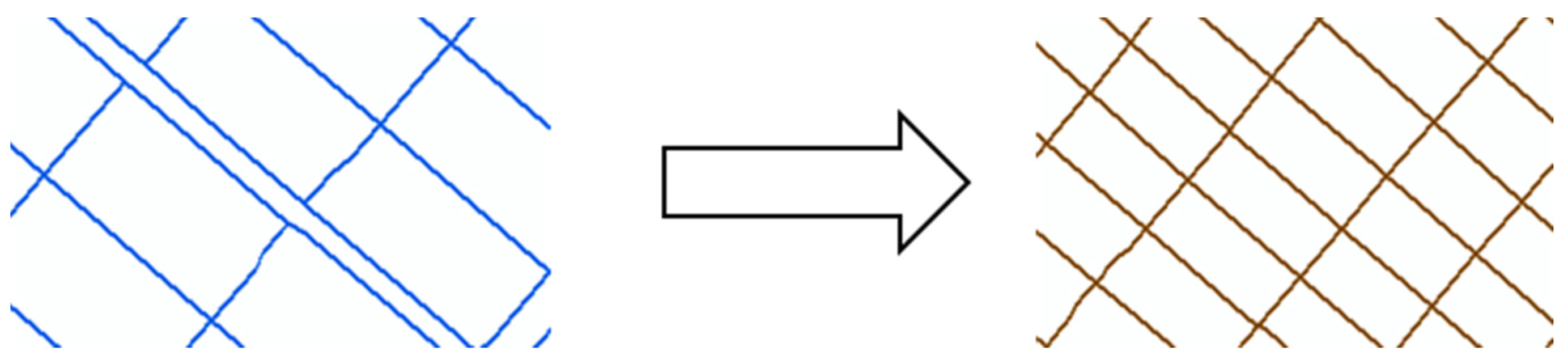
The obtained road network attributes of the Kowloon Peninsula of Hong Kong are shown in Table 3.
Table 3. OpenStreetMap road network attributes.
The value of the “lanes” attribute indicates the number of lanes in the road, including all lanes in a two-way road. For example, a two-way road with two lanes can be labeled as “lanes = 4”, where two lanes are used in each direction.
The value of the “shape” attribute indicates the shape of the line elements; in this study, the road network is folded lines.
The value of the “highway” attribute indicates the class and type of the road, and there are mainly the following categories:
(1)
Motorway: highway;
(2)
Trunk: trunk highway;
(3)
Primary: major roads;
(4)
Secondary: secondary roads;
(5)
Tertiary: third-class roads;
(6)
Residential: residential roads;
(7)
Unclassified: unclassified roads.
The contents of the road network data attribute table are shown in Table 4.
Table 4. Table of road network data attribute values.
OpenStreetMap data are contributed by community volunteers, so there may be an incomplete coverage of the map data, and at the same time, according to the research objectives of this paper, it is also necessary to carry out a secondary processing of the road network, so as to ensure that the adopted road network can be used to carry out the research on the identification of traffic black spots at road intersections.
The process of secondary processing of the road network mainly includes the following steps:
Road network connectivity processing: in some cases, the road network may have the problem of discontinuity, that is, some areas cannot be reached or can only be reached through longer paths, which will affect the recognition results of traffic black spots, so it is necessary to carry out connectivity processing.
Road network segmentation: road network segmentation consists in cutting the road network into small segments, which can be nodes, edges, or regions, which can improve the computational efficiency and accuracy of the traffic black spot recognition algorithm. In this study, the road network segmentation is performed at road network intersections.
Remove redundant road network lines. Turn two-way roads into unidirectional lines, circular intersections into unidirectional cross-connection-type lines, etc. Such treatment can simplify the road network, avoid repeated calculations, and unify the road representation.
Using MapGIS 10.6 software to process the road network, verify the road connectivity, and eliminate the disconnected roads, unconnected roads, and branch lines. Secondly, the redundant road network lines are deleted, so that the road network map used in this study can be initially obtained, and a road network processing example is shown in Figure 3, Figure 4 and Figure 5.
Figure 3. Deleting redundant branches.
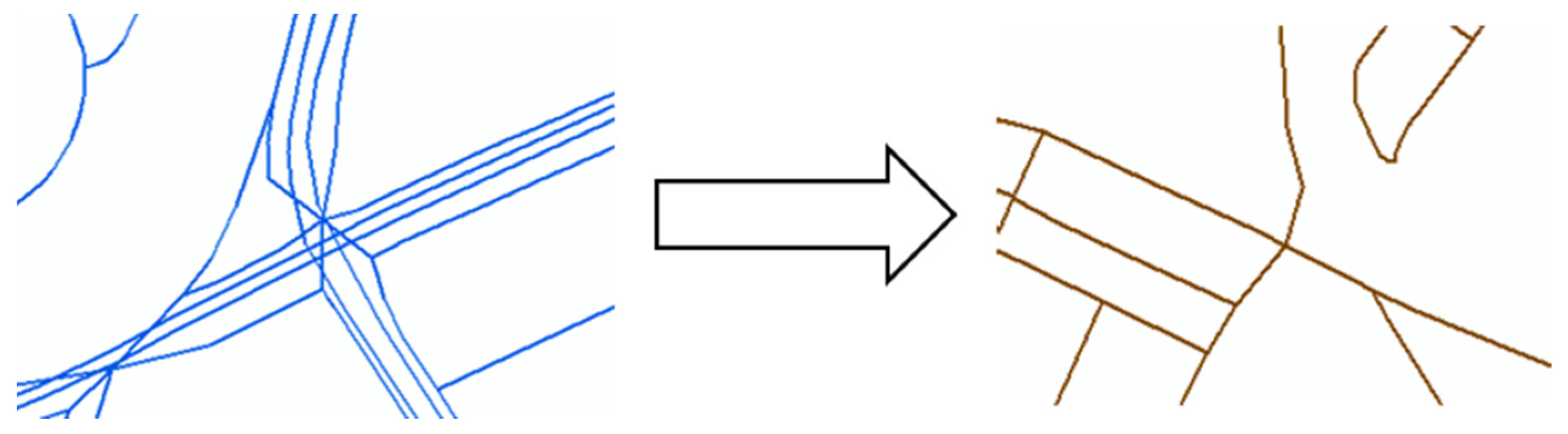
Figure 4. Example of road intersection treatment in Kowloon Peninsula.
Figure 5. Example of multi-lane treatment in Kowloon Peninsula.
Deleting redundant branch roads in the road network, as shown in Figure 3, simplifies the road network and does not interfere with the research experiments.
As shown in Figure 4, the complexity of roadway intersection routes in the roadway network is generally simplified to one adjacent route, with the roadway intersection becoming a simpler cross-connection type.
As shown in Figure 5, the two-way lanes in the road network are simplified into one-way lanes, while the lines are connected to form road intersections.
After processing the above steps, the road network map used in the experiment can be initially obtained, as shown in Figure 6.
Figure 6. Results of road network treatment in Kowloon Peninsula.
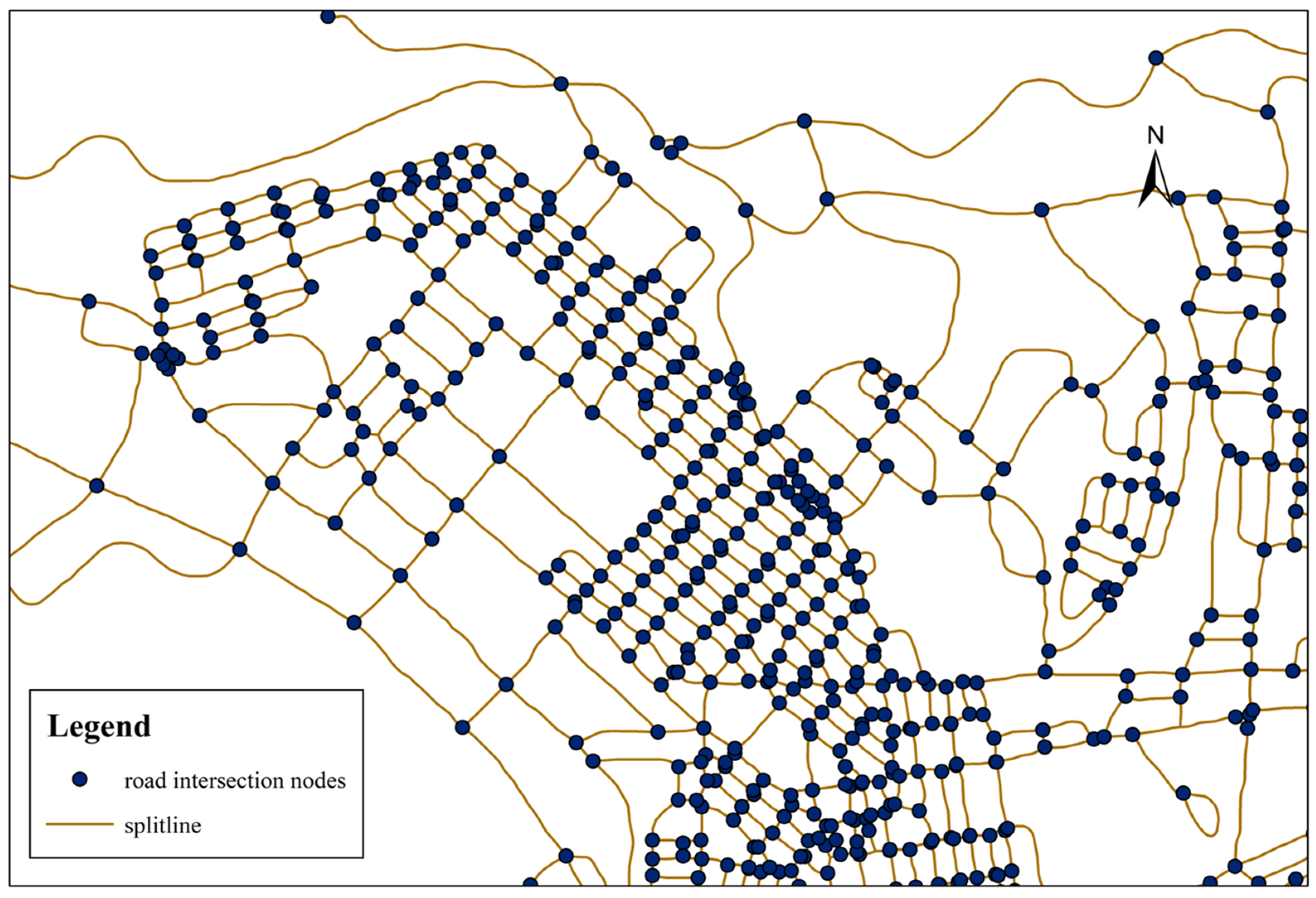
The road network shown in Figure 7 is processed using MapGIS software to interrupt intersectionality from road intersections to form road intersection nodes, and Figure 7 demonstrates the results of localized road intersection node processing in the Kowloon Peninsula area.
Figure 7. Illustration of the location of local road intersections in Kowloon Peninsula.
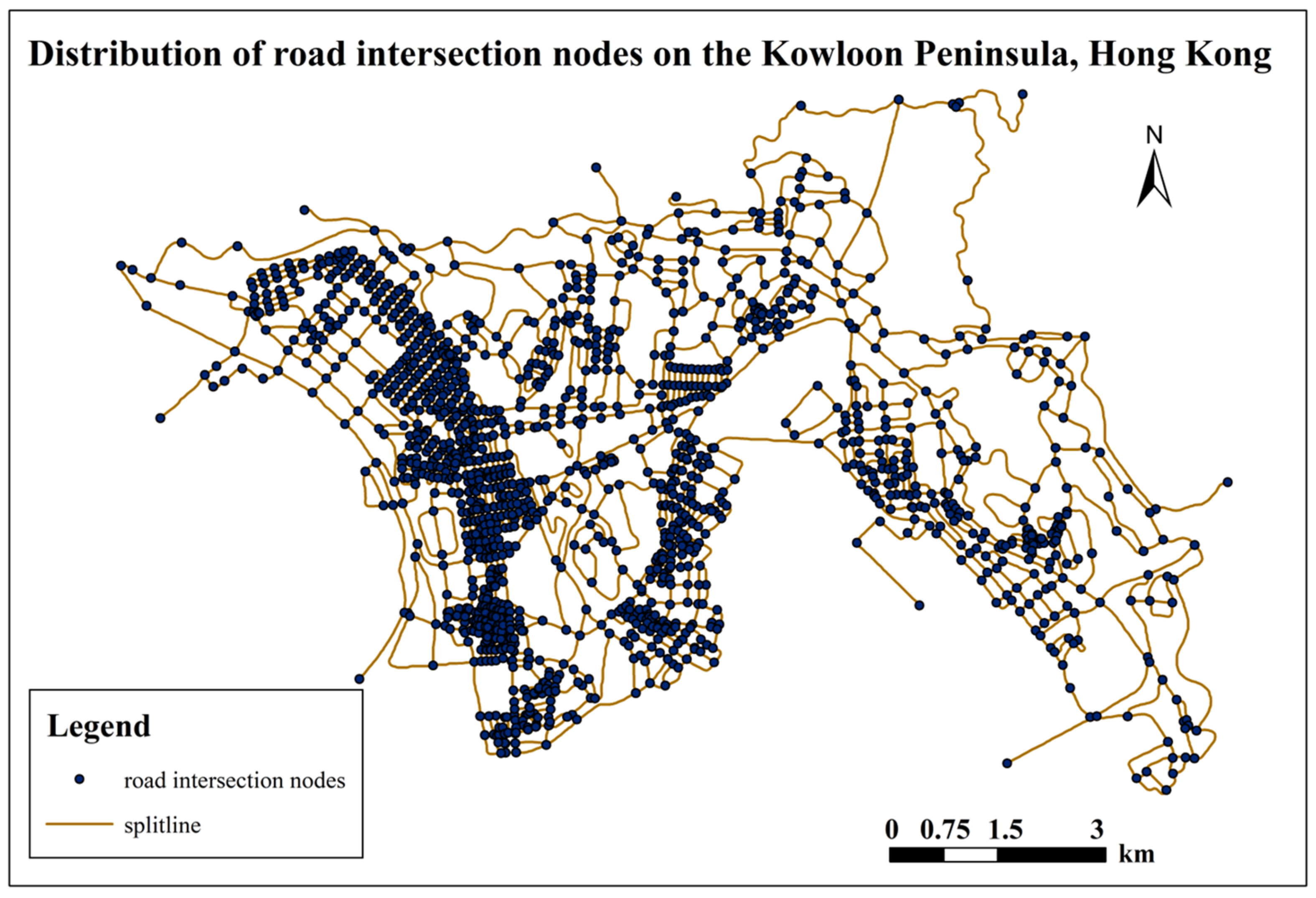
The road network road intersection nodes in the entire Kowloon Peninsula area were processed to obtain a total of 2519 intersections, and the results are shown in Figure 8.
Figure 8. Illustration of the location of the intersection at Kowloon Peninsula.
After the above steps, the final road network map and road intersection node location map used in this experiment are obtained.

3.2.2. Traffic Accident Data Acquisition and Processing

(1)
Traffic accident data acquisition
The traffic accident data used from 2014 to 2015 were obtained from the Hong Kong Traffic Management Department. The data attributes include latitude and longitude coordinates, weather conditions, and accident severity, etc., and there are a total of 10,392 entries.
The acquired traffic accident data attributes are shown in Table 5.
Table 5. Table of attributes of traffic accidents.
According to the research objectives of this experiment, focusing on selecting fid attribute, year attribute, latitude attribute, and longitude attribute, the content of the attribute table of traffic accident data is displayed, as shown in Table 6.
Table 6. Table of values of traffic accident data attributes.
(2)
Traffic accident data processing
The main purpose of the experiment is to remove the traffic accident data with missing latitude and longitude attributes, and it also includes some steps such as filling the missing values and processing the outliers (the latitude and longitude coordinates are not on the road network, etc.). After processing, a total of 8374 pieces of experimentally available traffic accident data were obtained.
A buffer zone will be established using MapGIS 10.6 with the road intersection node as the center of the circle, as shown by the black dot in Figure 9, with a radius of 100 m.
Figure 9. Illustration of road intersection buffers.
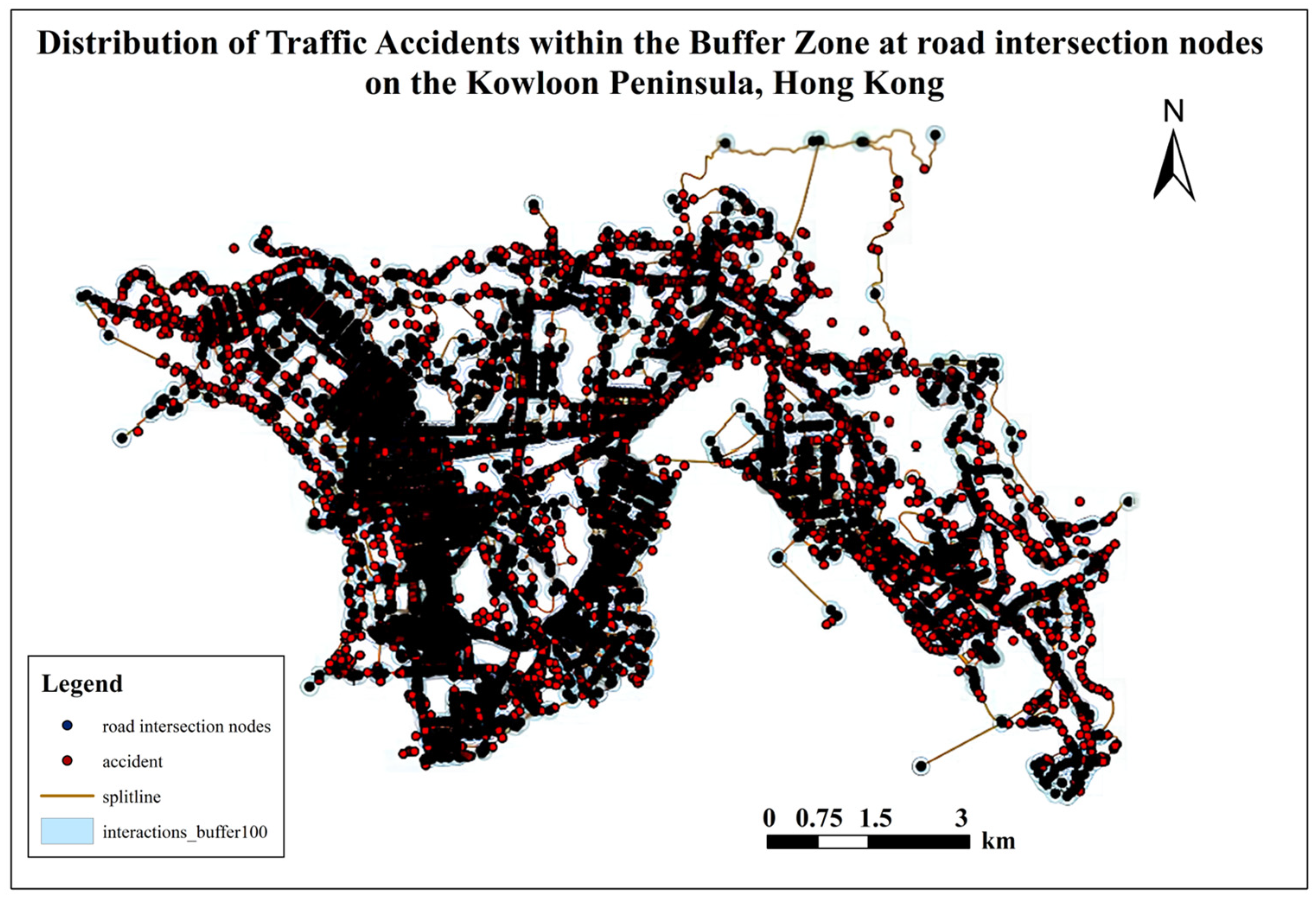
Then, combining the 8374 traffic accident data points, using MapGIS to import them into the established road intersection buffer and unify the coordinate system, the final results are displayed as shown in Figure 10.
Figure 10. Graphical representation of traffic accident data falling within the intersection buffer zone.
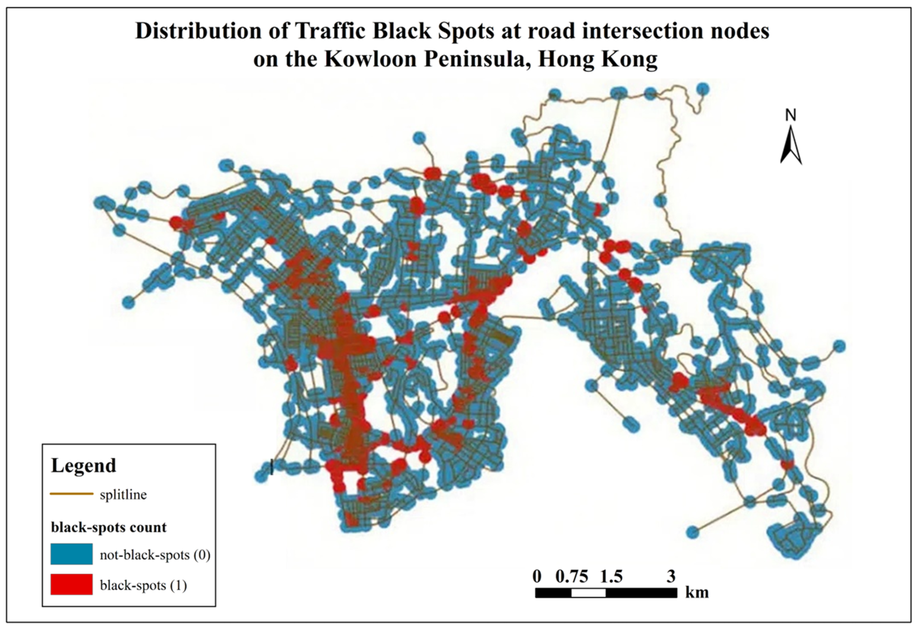
If the number of traffic accidents in this buffer zone exceeds twenty or more, this defines the road intersection as a traffic black spot. After counting, there are 584 traffic black spots in total, and the final results are displayed as shown in Figure 11, where the red nodes denote the traffic black spots, which are replaced by the number 1, and the blue nodes denote the non-traffic black spots, which are replaced by the number 0.
Figure 11. Distribution of traffic black spots.
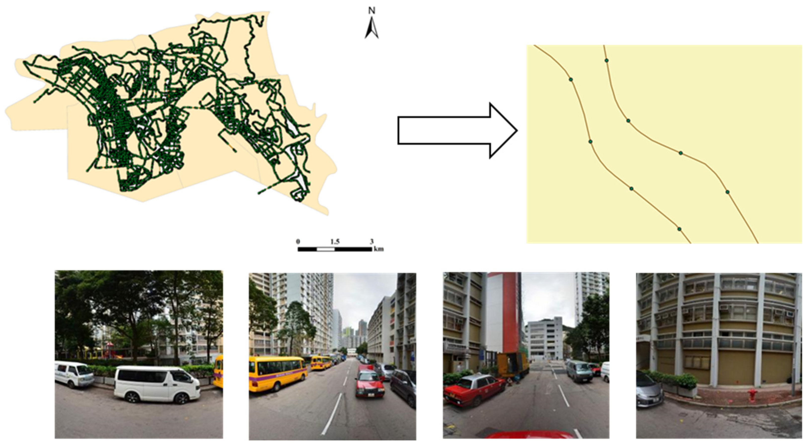
The MapGIS platform was also used to count the distribution of traffic black spots in the five districts of Kowloon Peninsula, as shown in Table 7.
Table 7. Table showing the number of traffic black spots distributed in various districts of the Kowloon Peninsula.

3.2.3. Streetscape Image Data Acquisition

In this study, we utilize the street view image data provided by the Tencent Street View platform to extract street-level road environment features. By analyzing the road network data, we selected a total of 8044 street view sampling points with an average sampling interval of about 100 m. Four images were captured at each sampling point with orientations of 0°, 90°, 180°, and 270°, constituting a 360° panoramic view to fully characterize the environment at each sampling point. We acquired a total of 32,176 street view images of Hong Kong’s Kowloon Peninsula, each with a size of 1024 × 1024 pixels. The final sampling point location map and the acquired street view images are shown in Figure 12, with the green nodes representing the street view sampling points.
Figure 12. Schematic diagram of sampling points of streetscape image.
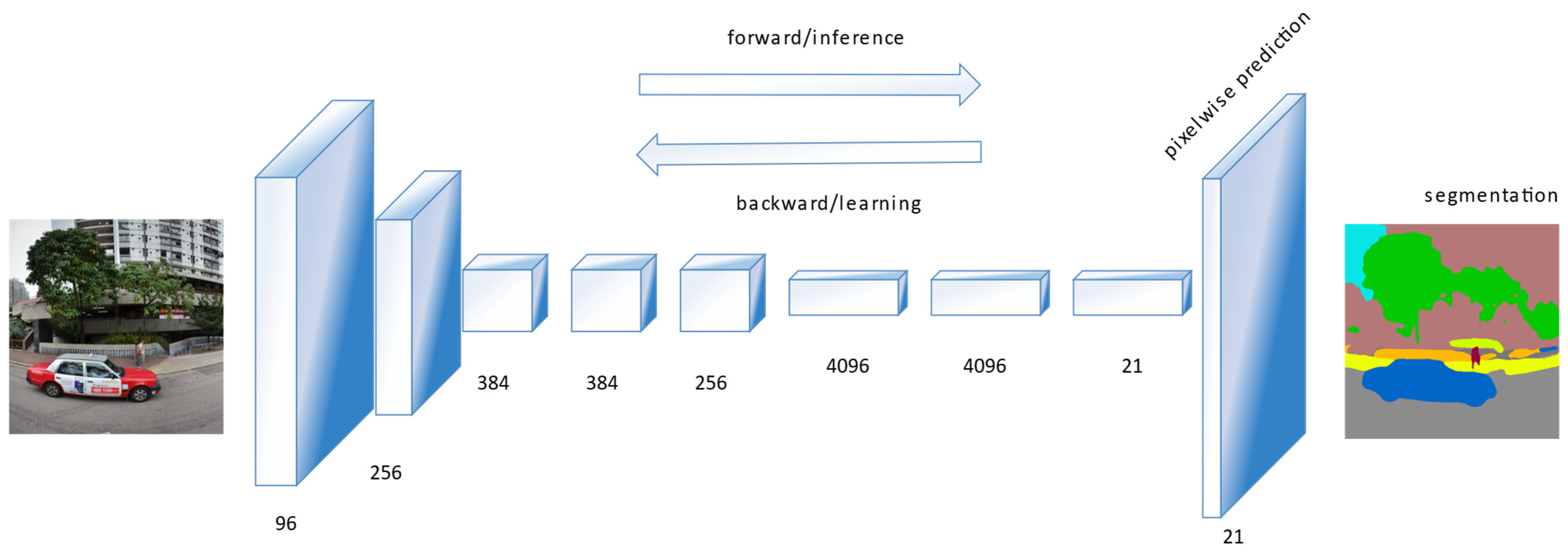
3.2.4. Streetscape Image Data Processing

In previous research, most scholars would apply traditional machine learning models (e.g., decision trees, convolutional neural networks) to classify street view images at the image level until the emergence of FCN [18] in 2015, which transforms the last layers of convolutional networks from the last few fully connected layers to the fully convolutional layers, realizing a breakthrough from image-level to pixel-level classification. In this study, we will use FCN, a classical semantic segmentation model, to recognize the pixels in street view images, including more than 100 features such as trees, buildings, billboards, roads, sidewalks, signals, and vehicles, and on the basis of which we will calculate the percentage of each feature in each group of street view images.
The basic structure of the entire FCN network is shown in Figure 13.
Figure 13. FCN semantic segmentation network graph.
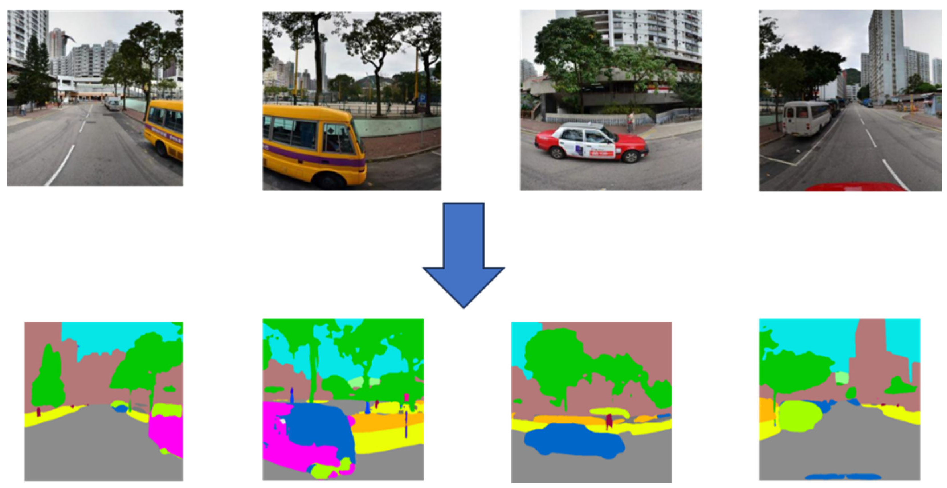
In this study, a deep learning fully convolutional network trained on the ADE_20K dataset, which has a pixel contrast accuracy of 81% in the training dataset [47], is used to perform semantic segmentation on the pixel level of the acquired street view images to obtain more than 100 street-level environmental features such as green trees, buildings, roads, and sky. The final input result image of the semantic segmentation model is at 512 × 512 pixels and the semantic segmentation result image is shown in Figure 14.
Figure 14. Graph of semantic segmentation results.
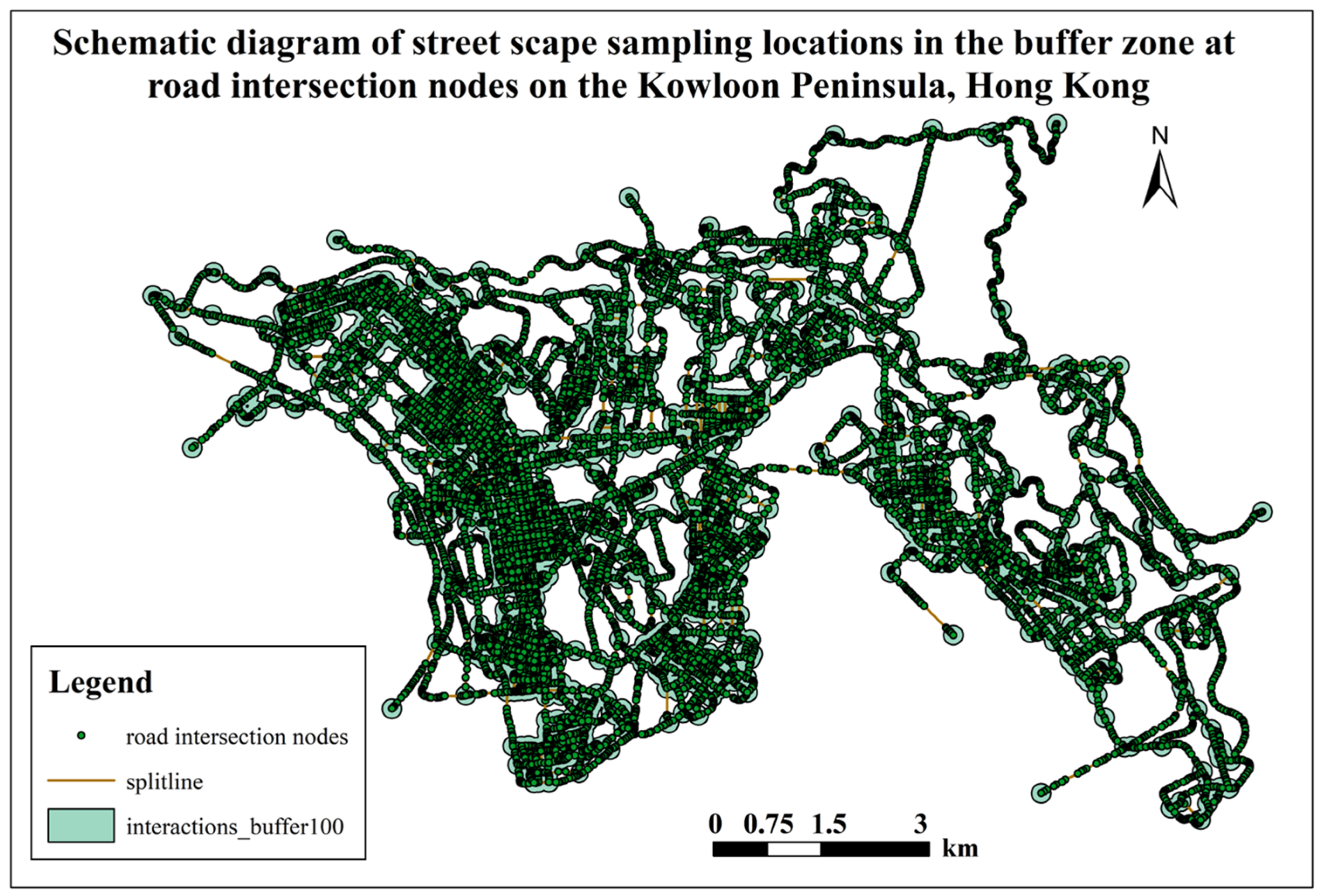
As can be seen from the result of semantic segmentation, in Figure 14, the model has a better recognition effect, but there is still a slight error. For large-scale street scene recognition, such an error is acceptable. At the same time, the model will also obtain a picture element feature percentage data table, the attributes of which are shown in Table 8.
Table 8. Semantic segmentation model element feature shared attributes.
The results of the feature occupancy of some elements of the semantic segmentation model for street scene images are displayed in Table 9.
Table 9. Feature share of some elements of the semantic segmentation model for streetscape images.
As shown in Table 9, the svid attribute is the unique number of the street scene sampling point; while each sampling point has four pictures, according to the different direct attributes to differentiate the direction, in the process of data processing, it is necessary to calculate the average of the four-picture occupancy of the same sampling point, to obtain the unique elemental feature occupancy data of each sampling point. At the same time, zero is assigned to the picture occupancy of the feature to avoid null values. The final elemental feature ratio of the semantic segmentation data of street view images for each sampling point is shown in Table 10.
Table 10. Feature share of data elements for semantic segmentation of streetscape images.
The coordinates of each sampling point are imported into the road intersection buffer established in the previous section, and the number of sampling points falling into the buffer and the percentage of each element’s characteristics are counted as a means of depicting the built environment of the road intersection, and Figure 15 shows the distribution of the sampling points of the streetscape in the road intersection buffer.
Figure 15. Distribution of sampling points within the buffer zone at road intersections.
The number of sampling points distributed in the buffer zone of roadway intersections was counted and the results are shown in Figure 16.
Figure 16. Statistics on the number of sampling points in the buffer zone of road intersections.
Statistical results show that each buffer has a sufficient number of sampling points, indicating that the results of semantic segmentation of street view images can be used to represent the built environment of road intersections in the study area, which lays the foundation for the smooth progress of the experiments on traffic black spot recognition.
Finally, the results of semantic segmentation of street scene images in each buffer are processed by data connection, filling, etc., and the final part of the built environment of some road intersections is shown in Table 11.
Table 11. Characteristic percentage of road built environment elements at road intersections.

4. Methodology

4.1. Machine Learning Models

4.1.1. SVM

SVM is an algorithm under a supervised learning model, commonly used in classification problems. The earliest SVM model is a linear classifier dedicated to binary classification, with a statistical theory foundation. The SVM method maps the sample space into a high-dimensional or even infinite-dimensional eigenspace (Hilbert space) through a nonlinear mapping p, so that a problem that is nonlinearly differentiable in the original sample space is transformed into a problem that is linearly differentiable in the eigenspace. Simply put, it is lift and dimension linearization. Due to classification, regression, and other problems, it is likely that the sample set in the low-dimensional sample space cannot be linearly processed, but in the high-dimensional feature space this can be achieved through a linear hyperplane linear division (or regression). Generally, while upgrading will bring the complexity of computation, the SVM method applies the expansion theorem of the kernel function and establishes a linear learning machine in high-dimensional feature space; therefore, compared with the linear model, not only does it almost not increase the complexity of the computation, but to a certain extent it also avoids the “dimensionality catastrophe”. Different SVMs can be generated by choosing different kernel functions, and the following four kernel functions are commonly used: (1) linear kernel function K x , y = x · y ; (2) polynomial kernel function K x , y = x · y + 1 d ; (3) radial basis functions K x , y = x y 2 d 2 ; (4) two-layer neural network kernel function K x , y = t a n h a x , y + b . Figure 17 is the construction flowchart of the SVM model for binary classification of traffic black spot recognition.
Figure 17. SVM model traffic black spot recognition classification model construction process.
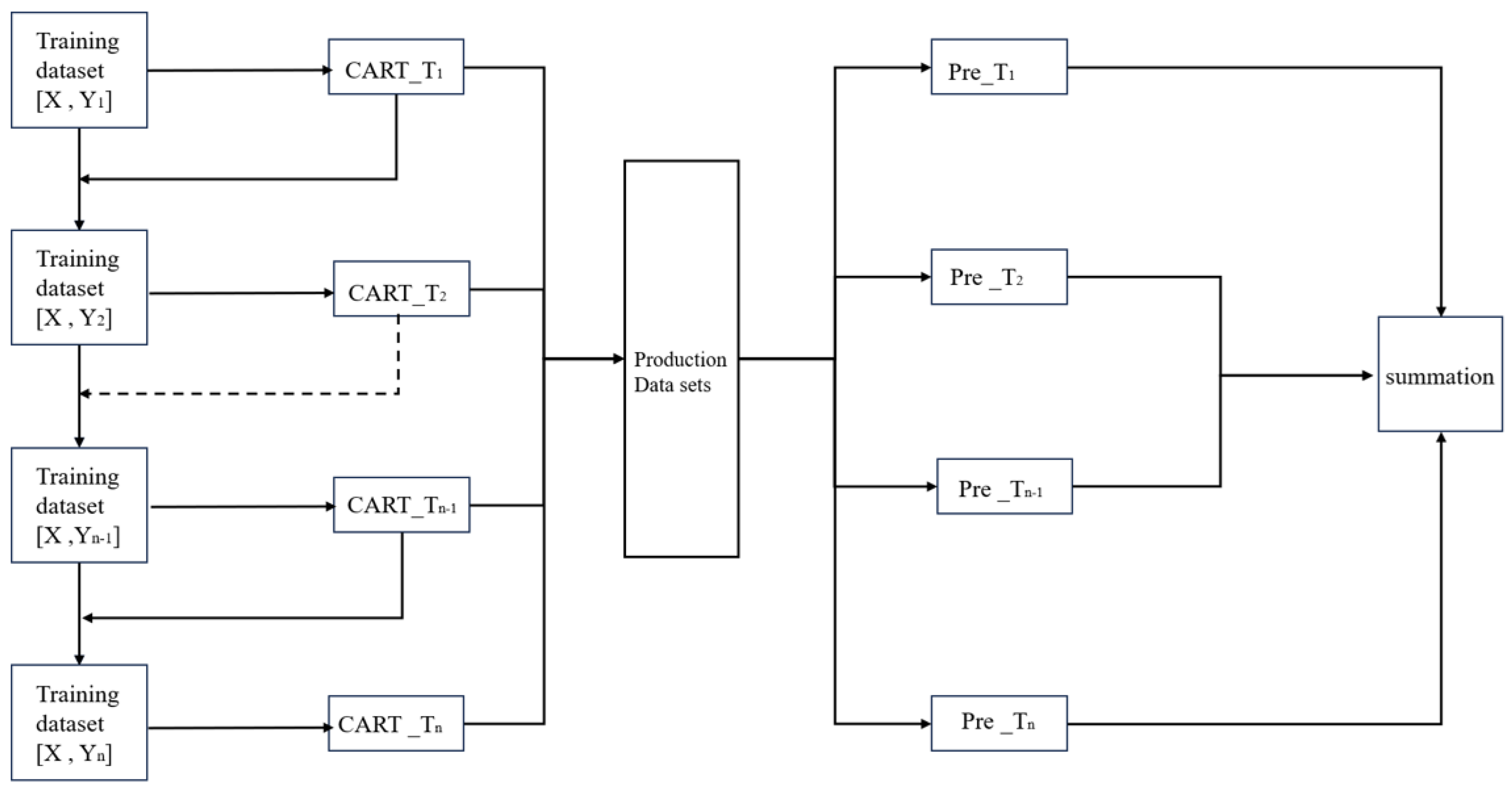
The SVM model is trained using data with selected features, and during the training process, appropriate parameters and kernel functions need to be selected to optimize the performance of the model. In this process, the model parameters need to be selected, and the more important parameters are selected as follows:
(1)
The choice of kernel function. Depending on the different SVM model kernel functions, the accuracy of the SVM model will be different; generally, it will be a linear kernel function, Gaussian kernel function, Sigmoid kernel function, and so on;
(2)
Optimization of kernel parameters. The main parameters are the kernel parameter g and the penalty factor c. The penalty factor indicates the importance of misclassification, and the parameter g indicates the size of the impact of a single sample, and the smaller the value, the greater the impact.
The specific description of the model parameters is shown in Table 12.
Table 12. Important parameters of the SVM algorithm model (described in words).
The SVM function package in the machine learning Sklearn toolkit was used to model the SVM algorithm, and the model accuracy was higher when the kernel function was chosen to be linear, in addition to the other parameters of the algorithmic model (Table 13), which were appropriately tuned using the grid search method.
Table 13. Selection of model kernel function for SVM algorithm.
According to Table 14, the accuracy of the model is high when the kernel function is chosen to be linear. The appropriate kernel function is chosen to find the optimal classification hyperplane, and the support vector set of each sample feature is obtained to form the discriminant function of classification.
Table 14. Values of important parameters of the SVM algorithm model (direct textual description).

4.1.2. GBDT Model

GBDT is a common basic machine learning algorithm based on boosting iterative decision trees that can be used for classification, regression, and other problems. The steps of the algorithm first train a decision tree with an initial sample, and then train the next decision tree based on the residuals of the previous decision tree, thus gradually reducing the iterative residuals, thus improving the iterative results and finally constructing a new combinatorial model. When all the convergence criteria are satisfied, all the base models are obtained. In the GBDT classification algorithm, the final output is discrete categories rather than continuous values, so we cannot fit the category output error directly from the output categories. To solve this difficulty, we fit the loss function using a method similar to the log-likelihood loss function used in logistic regression. The dataset of this experiment has a relatively large number of features, and the traditional linear model cannot achieve a better classification effect. GBDT, as one of the representative models of integrated learning, consists in training multiple weak learners and synthesizing their classification results to form a strong learner. Figure 18 shows the flowchart of the construction of the GBDT model for the binary classification of the traffic black spot recognition.
Figure 18. GBDT traffic black spot identification classification model construction process.
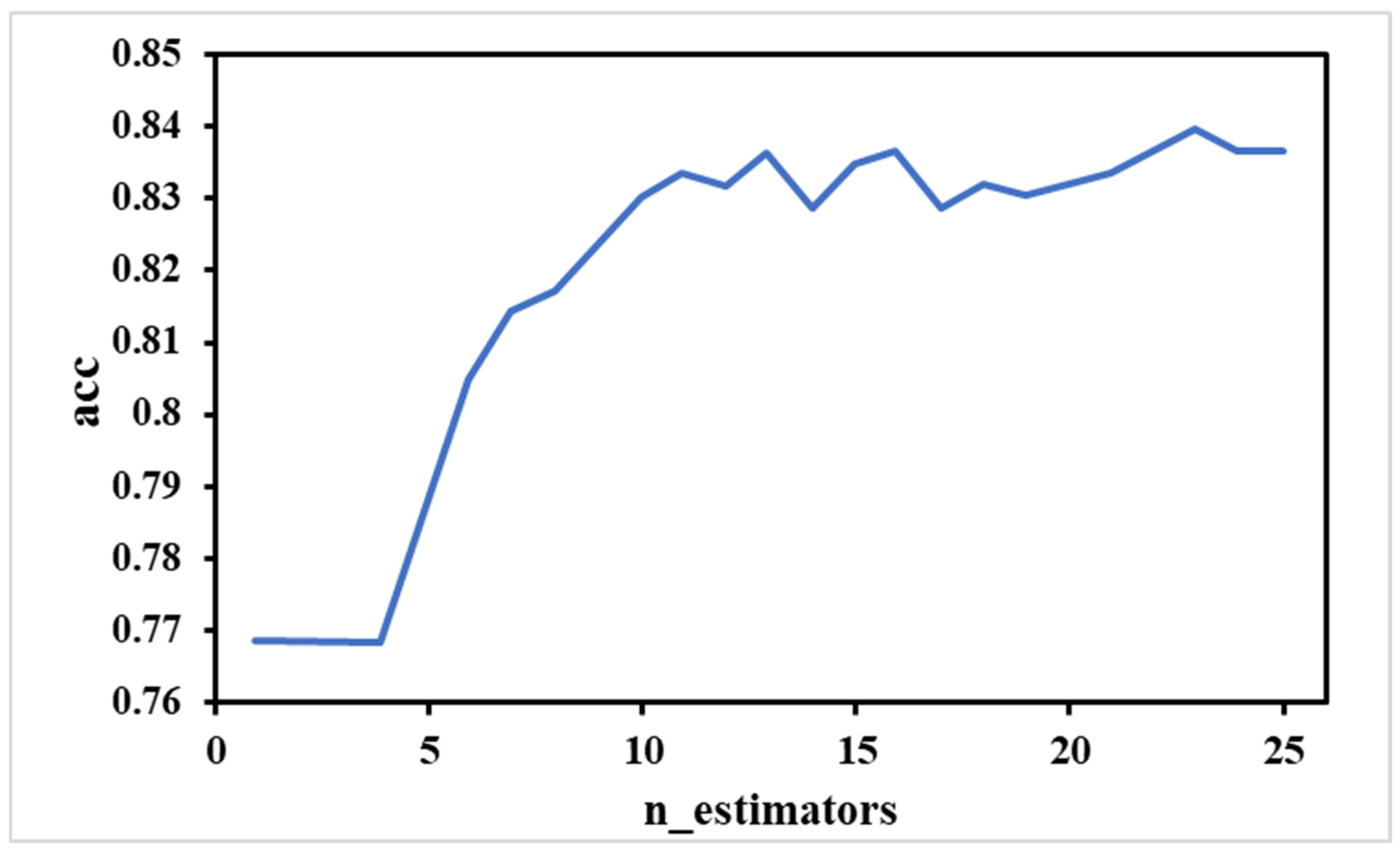
Figure 18 consists of multiple weak learners. X represents the feature attributes, Y represents the prediction results of the weak classifiers, and the results of multiple weak learners are combined to obtain the final classification results.
The traffic black spot recognition model is constructed using the GBDT model, which is an integrated learning method based on a decision tree, and its main idea is to construct a strong classifier by combining multiple weak classifiers. When building the GBDT model, it is necessary to select the hyperparameters such as the depth of the decision tree and the number of leaf nodes, as well as to adjust the parameters such as the learning rate and the loss function. The selection and description of model parameters are shown in Table 15.
Table 15. Important parameters of the GBDT algorithm model.
Gradient Boosting Classifier in the machine learning Sklearn toolkit was used to model the GBDT algorithm, with loss as the loss function, and then 2519 data points were randomly divided into test and validation sets, and the parameters of the algorithmic model were appropriately tuned using the grid search method, including the parameters of n_estimators, max_depth, and so on.
As shown in Table 16, the values of the loss parameter are set to deviance and exponential, respectively, and it can be seen that the model is slightly more accurate when the value of the loss parameter is set to deviance.
Table 16. Comparison table of loss fetch value tuning reference.
According to Figure 19, the accuracy of the model is higher when the n_estimators parameter in the GBDT model is set to 23.
Figure 19. GBDT grid search tuning map.
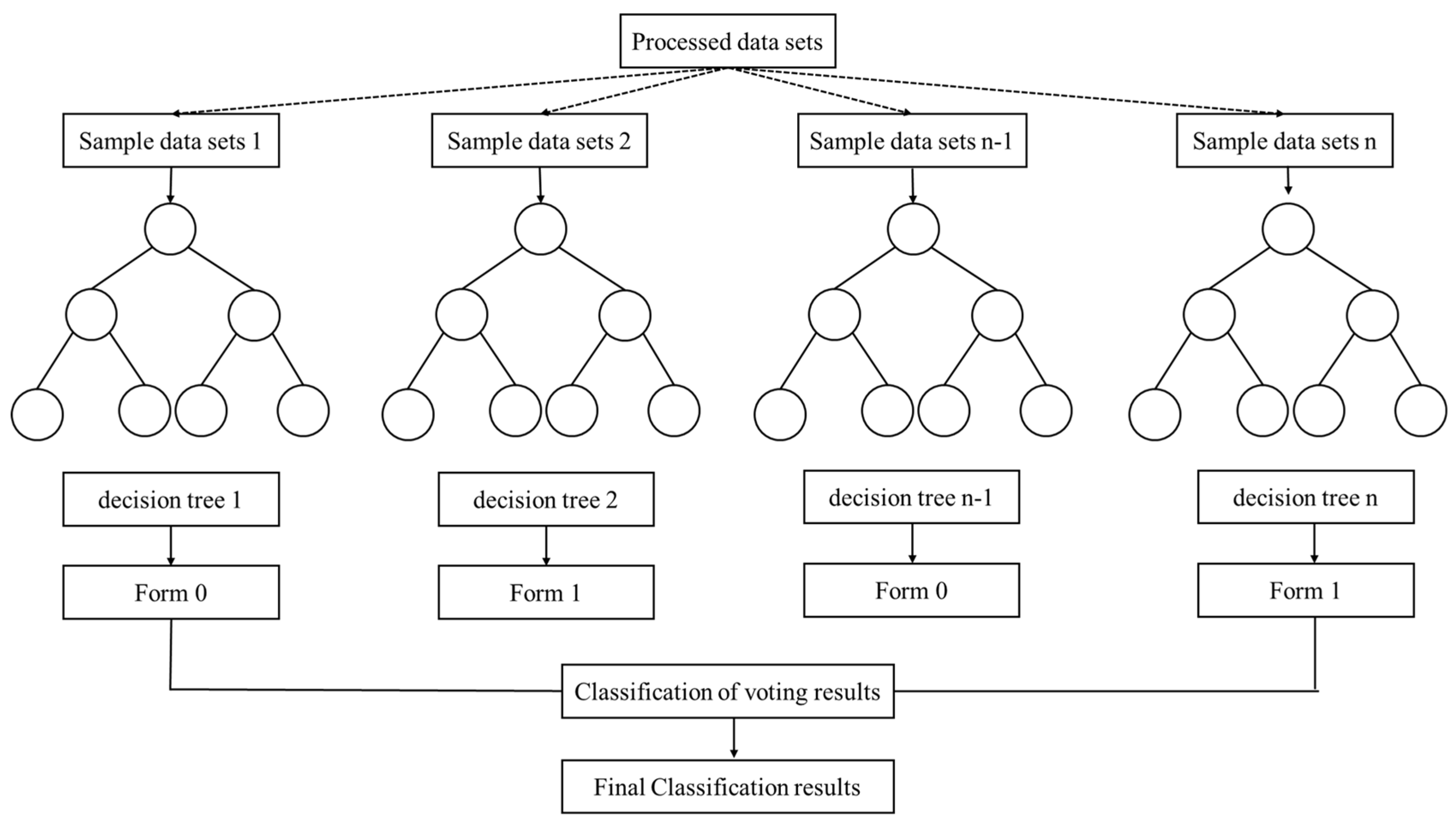
Moreover, the results of the grid search method show that the accuracy of the model is better when the other parameter, max_depth, is set to 7 and when min_samples_leaf is set to 1. Table 17 shows some of the parameter settings of the GBDT model, on the basis of which the GBDT model is used for the identification study of traffic black spots.
Table 17. Values of some parameters of the GBDT model.

4.1.3. Random Forest

Random forest is one kind of cluster classification model, which consists in building a forest in a random way. The forest consists of a significant number of decision trees, and there is no association between each decision tree. After obtaining the random forest model, when a new sample enters the random forest for each decision tree to judge, the bagging collection strategy is relatively simple, for classification problems usually use the voting method to obtain the category with most votes for the final model output. Firstly, from the original training dataset, the bootstrap method is applied to randomly draw k new self-help sample sets with put-back, and from this, k decision trees are constructed, and the samples that are not drawn each time make up K out-of-bag data. Second, there are n features, and mtry features are randomly drawn at each node of each tree, and by calculating the amount of information embedded in each feature, one of the features with the most classification ability is selected for node splitting. Third, each tree is maximally grown without any clipping. Fourth, the generated multiple trees are formed into a random forest, which is used to classify the new data, and the classification result is based on how many tree classifiers are voted for. For classification problems, the random forest model can naturally handle most classification tasks, and it is a natural and nonlinear classification model. Figure 20 shows the flowchart of the construction of the random forest model for binary classification of traffic black spot identification.
Figure 20. Random forest traffic black spot identification classification model construction process.
Next, we discuss model training using the random forest algorithm. Random forest is an integrated learning method that combines multiple decision trees to form a more accurate classifier. Some parameters need to be set during training, such as the number of trees, the maximum depth of each tree, and the minimum number of samples for leaf nodes, as shown in Table 18.
Table 18. Important parameters of random forest.
In the tuning process of random forest models, there are several principles:
Training set random sampling selection. In this study, the bagging method is chosen for sampling, which can prevent overfitting and at the same time has a relatively fast training speed.
Selection of training objective function. There are mainly two kinds, information gain and Gini coefficient; the Gini index tends to select features with more values as split features, while the information gain index easily causes overfitting when using high latitude data. According to the data of this experiment, the Gini coefficient index is selected.
Parameter selection. The max_depth parameter indicates the maximum depth of the tree, generally set as max_depth = 3, and then to try to increase the depth, the min_samples_leaf parameter indicates the minimum number of samples specified to be contained in each leaf node. If this parameter is set too low it will cause overfitting, so generally it is set as min_samples_leaf = 5, and followed by up and down adjustment.
In this paper, we use the Random Forest Classifier in the machine learning toolkit to construct the random forest algorithm model, which can set a series of parameters to tune the model, we use the logloss function for the calculation of the loss function, and in this process, randomly classify the test set and validation set on 2519 pieces of data, and we use the grid search method. The algorithm model is tuned, after which the max_depth parameter is set to 13 and the max_features parameter is set to 46. Figure 21 shows the tuning diagram of the random forest model parameter n_estimators as set to 15, and Table 19 shows the values of some parameter settings of random forest.
Figure 21. Random forest grid search tuning parameter map.
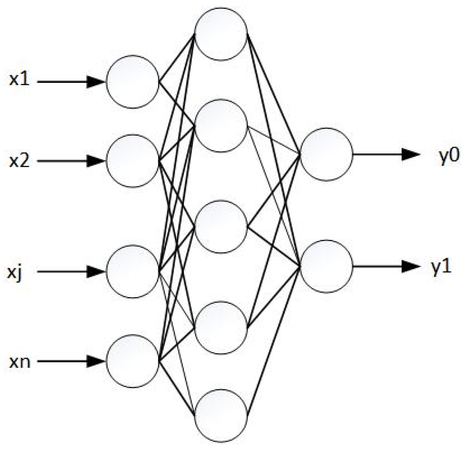
Table 19. Values of some important parameters of random forest.

4.1.4. Fully Connected Neural Network

Figure 22 is a flowchart of the construction of a fully connected neural network model for the binary classification of traffic black spot identification.
Figure 22. The process of constructing a classification model for traffic black spot recognition by a fully connected neural network.
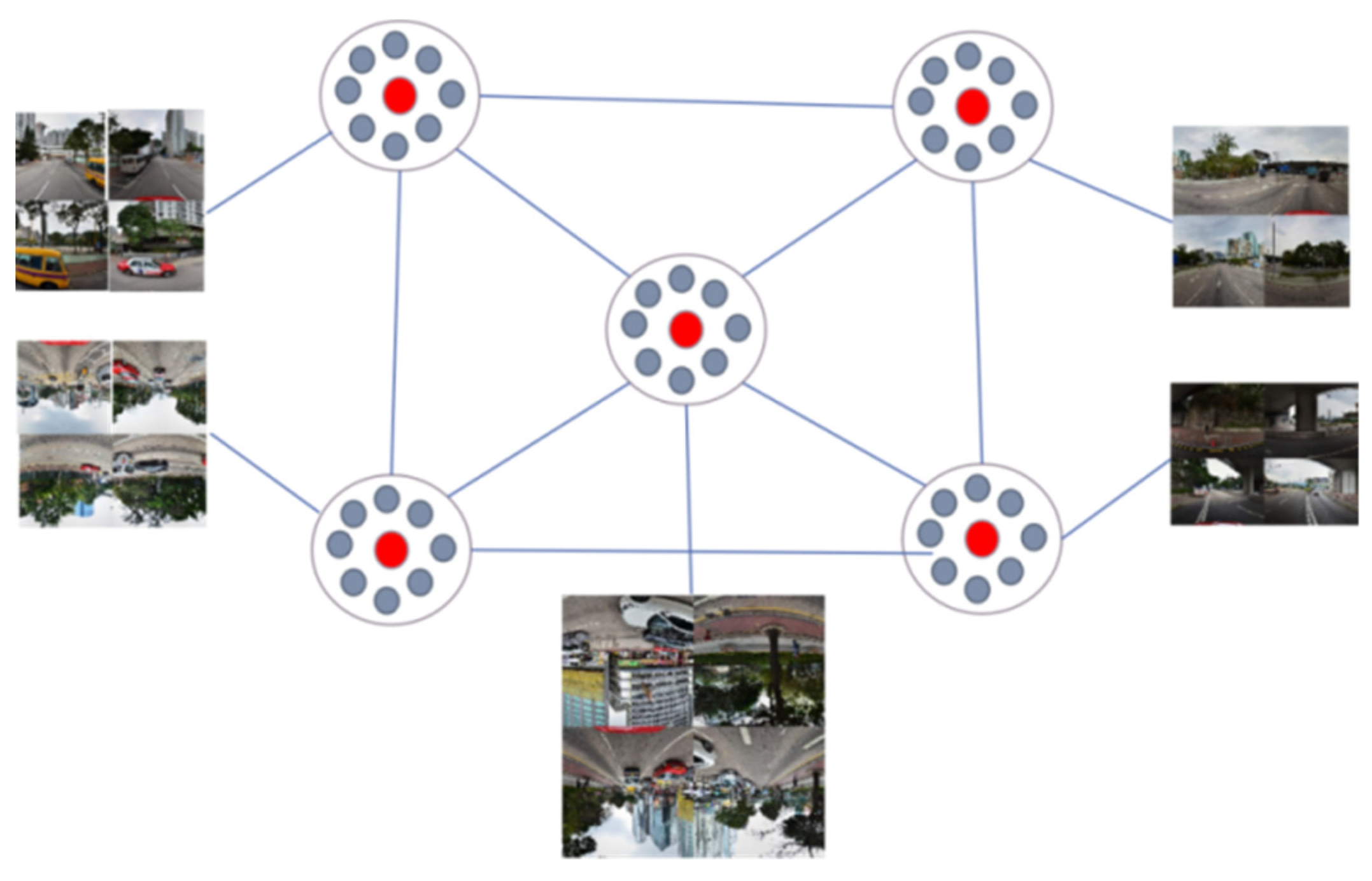
Figure 22 consists of an input layer, a hidden layer, and an output layer, where x represents the feature attributes and y represents the classification results of traffic black spots.
A fully connected neural network model is constructed, and data are fed into the model to train the model for the classification task. A fully connected neural network can consist of multiple hidden layers, each layer containing multiple neurons and each neuron being connected to all the neurons in the previous layer. Some parameters need to be set during training, and after network tuning, some of the hyperparameters of the fully connected neural network proposed in this study are set at the following values:
(1)
Input layer vector dimension: 139 features of each intersection semantic segmentation will be input;
(2)
Number of hidden layers: the number of hidden layers is three;
(3)
Neurons: the neurons of the three hidden layers are 79, 17, and four, respectively;
(4)
Activation function: the activation function is chosen as ReLU, which is less likely to have gradient explosion or gradient disappearance;
(5)
Learning rate: the learning rate is between 0.005 and 0.01;
(6)
Back-propagation algorithm: after the neural network calculates the error according to the error function in the process of iteration. It needs to return the result to the end of input weight adjustment, which needs to consider the model effect and speed. In this study, Adam’s algorithm is chosen as the back-propagation algorithm for this model.
The values of some parameter settings of the fully connected neural network are shown in Table 20.
Table 20. Hyperparameter settings for fully connected neural networks.

4.2. Traffic Black Spot Recognition Model Construction Based on Graph Convolutional Neural Network Model (GCNN)

In this experiment, roads can be considered as nodes of the graph, and connections between neighboring roads are considered as edges of the graph. Then, the road features from the street view image data source can be input into the GCNN as node features. With the GCNN model, the following operations can be performed:
(1)
Neighbor node feature aggregation: the GCNN model can fuse the information between adjacent roads by aggregating the neighbor node features of each node. This allows for the features of neighboring roads to be used to better portray the urban built environment;
(2)
Contextual information learning: the GCNN model can learn the contextual information of each node, including the attributes, shapes, and traffic flows of neighboring roads. This helps to synthesize the relationship between roads to further portray the urban built environment;
(3)
Feature representation learning: the GCNN model can learn the representation of road features through multi-layer convolutional operations. Each GCNN layer can extract more advanced feature representations to capture more complex information about the urban built environment.
In the following, specific steps are described for the study of traffic black spot recognition at road intersections using the GCNN model.
(1)
Introduction of the dataset
This experiment requires the use of street view image semantic segmentation data and the corresponding road intersection data. There are 2519 intersections in total. The intersections are mainly divided into two categories: one is traffic black spot intersections and the other is non-traffic black spot intersections. Each intersection is connected to at least one other intersection, and the connectivity information between the 2519 intersection data points is obtained through Python data analysis. Each intersection is treated as a graph node, the connection of adjacent road intersections is the edge of the graph, the street view semantic feature information of this intersection is treated as the node information of the corresponding node, and there are 139 node features, and the value is the percentage of this feature in the image of this intersection, and the neighbor matrix is constructed by obtaining the adjacency table based on the connectivity between nodes to obtain the structure of the graph network, as shown in Figure 23, where the red color represents the intersections, and the gray color represents street view image sampling points. The final data form is as follows:
Figure 23. Structure of the network of streetscape images and roadway intersection composition maps. (The red nodes represent the identified nodes and the blue nodes represent the neighbors of the nodes).
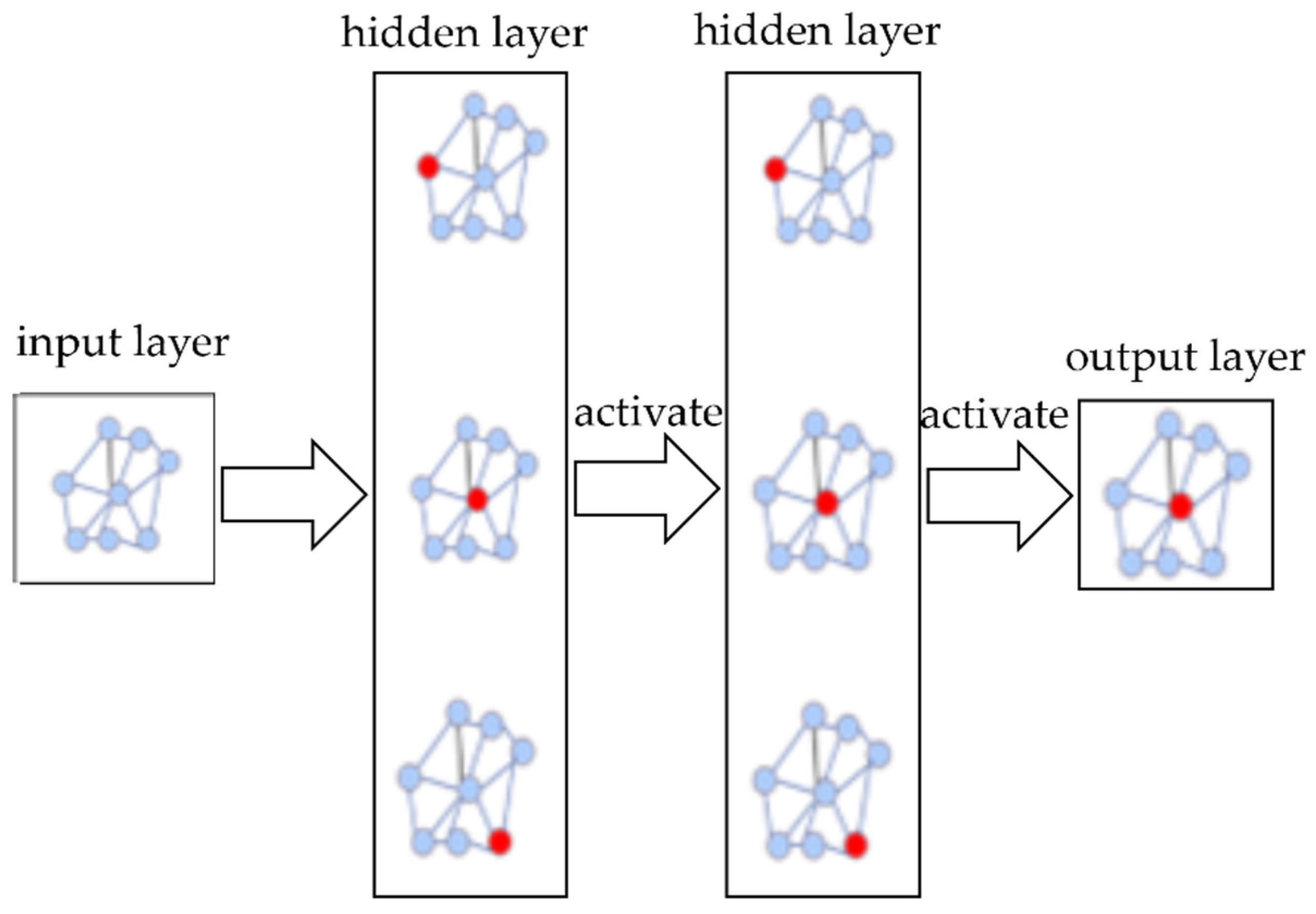
(1)
x: node features with dimension 2519 × 139 and type np.ndarray;
(2)
y: node corresponding labels, including two categories (traffic black spots and non-traffic black spots), np.ndarray;
(3)
Adjacency: adjacency matrix, dimension 2519 × 2519, type scipy.sparse.coo_matrix;
(4)
train_mask, val_mask, test_mask: the same mask as the number of nodes, which is used to classify the training set, validation set, and test set. When the node belongs to the training set or validation set or test set, the corresponding position is True, and otherwise it is False.
In GCNN node classification, how to choose and construct the feature matrix and adjacency matrix is crucial, because they directly affect the performance of the model.
(2)
Construction of the GCNN model
First of all, the data should be processed to obtain the node features and labels, adjacency matrix, training set, validation set, and test set. To normalize the data, to increase the self-connections, and to perform the definition of the graph convolution layer, the node input dimensions are 139 dimensions, the output is two dimensions, no bias is used, and at the same time, since the adjacency matrix is a sparse matrix, the sparse matrix multiplication method is used. Defining the graph convolution model, the hidden layer has a total of two layers, as shown in Figure 24.
Figure 24. Graph convolutional neural network model construction. (The red nodes represent the identified nodes and the blue nodes represent the neighbors of the nodes.)
(3)
Selection of GCNN model parameters
PyTorch-Geometric is a PyTorch-based graph neural network library specialized in processing graph network structures. It provides a series of tools for processing graph data, including data loading, data preprocessing, graph convolutional neural network model construction, model training, and model evaluation.
In this experiment, PyTorch, as well as the graph neural network library PyTorch-Geometric (PYG), are used. The Adam function is used for gradient descent, the loss function is used for the computation of the loss value, and the activation function is used for the calculation of the loss value by using ReLu. The hyperparameters are optimized, and the definitions of the hyperparameters are shown in Table 21.
Table 21. Graph convolutional neural network (GCNN) hyperparameter values.

5. Experimental Results and Analysis

5.1. Indicators for Model Evaluation

The data partitioning is kept consistent for all machine learning models and is divided into a training set and a test set. This ensures the comparability of the experimental results. When constructing the algorithmic model, all the sample data (a total of 2519 entries, each with 139 features) in the two categories (traffic black spots and non-traffic black spots) are randomly divided into 80% as the training set and 20% as the test set.
The main evaluation metrics commonly used in machine learning classification models are the following: (i) Accuracy; (ii) Precision; (iii) Recall; and (iv) F1_score; these metrics can help us evaluate the performance of the algorithm in different situations as well as provide valuable feedback when improving the algorithm. A confusion matrix is a matrix used to evaluate the performance of classification algorithms. In the binary classification problem of traffic black spot recognition at road intersections, the confusion matrix is a 2 × 2 matrix that contains the values True Positive (TP), False Positive (FP), True Negative (TN), and False Negative (False Negative, FN).
(1)
Definition of “Accuracy”: the ratio of the number of correctly categorized samples to the total number of samples. Accuracy is one of the most commonly used evaluation indices for classification models, but for the case of data imbalance, the accuracy may be misleading, and the expression is:
Accuracy = T P + T N T P + T N + F P + F N
(2)
Definition of “Precision”: the proportion of samples classified as positive that are truly positive. Precision is the evaluation of the ability of the classifier, i.e., the proportion of truly positive samples among all the samples determined as positive by the classifier, expressed as:
Precision = T P T P + F P
(3)
Definition of “Recall”: the proportion of all positive samples that are correctly categorized as positive samples. Recall is an index for evaluating the ability of a classifier to detect positive samples, i.e., the percentage of positive samples that can be detected by the classifier out of all real positive samples, expressed as:
Recall = T P T P + F N
(4)
Definition of F1 Score (F1 _ score ): the F1 value is a metric that combines precision and recall, i.e., the reconciled average of precision and recall. The higher the F1 value, the better the classification performance of the model, and the expression is:
F 1 _ score = 2   Precision     Recall Precision   +   Recall
In the experiments of this paper, the precision rate represents the proportion of real traffic black spots among the number of all judged traffic black spots; the recall rate represents the ability of the maximization model to find all traffic black spots in the dataset, i.e., the proportion of the number of correctly judged traffic black spots to the proportion of the actual number of all traffic black spots; and the F1 score is a combination of the two metrics of the precision rate and the recall rate, and the higher the value of the F1 score, the better the classification performance of the model.
The data are randomly assigned and the ratio of data in the training set and test set is 4:1. SVM, GBDT algorithm, random forest algorithm, and fully CNN methods are utilized for training and evaluation of the data.

5.1.1. Evaluation of SVM Model

Table 22 demonstrates that the average Accuracy was 81.14%, the average Precision was 74.12, the average Recall was 63.08%, and the average F1 score was 41.86%. The average Loss value was 6.513, the maximum Loss value was 7.346, the minimum Loss value was 5.658, and the standard deviation of Loss value std was 0.269.
Table 22. Different model evaluation metrics and loss function values.

5.1.2. Evaluation of GBDT Model

Table 22 demonstrates that the average Accuracy was 85.58%, the average Precision was 85.02%, the average Recall was 74.32%, and the average F1 score was 663.99%. The average Loss value was 4.636, the maximum Loss value was 5.795, the minimum Loss value was 3.741, and the standard deviation of Loss value std was 0.430.
The values of the loss function for the GBDT model, with loss values reaching an average of 4.6 per round, represent a reduction in loss values relative to the SVM model.

5.1.3. Evaluation of Random Forest Model

Table 22 demonstrates that the average Accuracy was 87.19%, the average Precision was 86.12%, the average Recall was 79.07%, and the average F1 score was 73.06%. The average Loss value was 3.725, the maximum Loss value was 4.928, the minimum Loss value was 2.738, and the standard deviation of Loss value std was 0.335.
The values of the loss function for the random forest model, with the loss values reaching an average of 3.7 per round, represent a significant decrease relative to the SVM model.

5.1.4. Evaluation of Fully CNN Models

Table 22 demonstrates that the average Accuracy was 84.54%, the average Precision was 83.04%, the average Recall was 73.57%, and the average F1 score was 68.09%. The average Loss value was 4.884, the maximum Loss value was 5.973, the minimum Loss value was 3.634, and the standard deviation of Loss value std was 0.421.
From the specific values of the evaluation index of the fully connected neural network model, it can be found that the accuracy of the fully connected neural network model reaches 84%, and there is a decrease in the accuracy relative to that of the random forest model, because the deep learning model is more prone to overfitting due to the limitation of the amount of data, and the value of the F1 score index reaches 68%, and in general, as the most basic aspect of the deep learning field of the network model, the fully connected neural network model also shows better performance.

5.2. Comparative Results and Analysis of Machine Learning Model Performance

In the study of traffic black spot recognition for each road intersection, it was found that, among the four models, namely SVM, GBDT, RF, and fully connected neural network, the random forest model was the most effective for traffic black spot recognition, with an accuracy rate of 87%, and at the same time the value of the loss was relatively small, and the results of the evaluation of the various models are shown in Table 23, which demonstrates that it is possible to utilize the characteristics of the built environment of the roads at each road intersection to conduct the study of traffic black spot recognition by means of the results of the above experiments.
Table 23. Comparison of the results of the four model constructions.
The results of the above models show that, in the case of only considering the built environment of urban roads with only a single intersection, the random forest model is the most effective, with an accuracy rate of about 87%, while the precision rate and the recall rate both reach more than 80% at the same time, and the accuracy rates of the other models reach more than 80% as well. The above information fully exemplifies the feasibility of using street view images to identify the traffic black spots at road intersections.
However, all of the above machine learning models only recognize the road intersections in each study area as an independent individual, and have not yet considered the influence of the interconnections between the road intersections on the recognition of traffic black spots; therefore, in the next section, we will analyze the spatial correlation of the traffic black spots to show that there is a clustering effect between the traffic black spots.

5.3. Spatial Correlation Analysis of Traffic Black Spots

Spatial correlation is the correlation between phenomena or variables in geographic space. It involves the factor of geographic location and examines whether there is a correlation or similarity between neighboring regions in geographic space.
In previous studies, the spatial distributions of traffic black spots are generally not considered to be spatially independent of each other, and the probability of them being the same traffic black spot is higher when the physical environments are very similar. Therefore, this paper will analyze the spatial correlation of traffic black spots at road intersections in the Kowloon Peninsula region of Hong Kong through the use of spatial analysis methods such as the global Moran’s I.
Spatial correlation analysis of traffic black spots at road intersections in the Kowloon Peninsula region of Hong Kong can reveal their geospatial distribution patterns, clustering, and the degree of association with other factors. This is of great significance for transportation planning, traffic safety, and traffic management, and helps to improve the efficiency and safety of the transportation system.

5.3.1. Global Moran’s I

Global Moran’s I is a commonly used statistical index that can be used to measure the overall spatial correlation of traffic black spots at road intersections in Kowloon Peninsula, Hong Kong.
In this section, the study takes the Kowloon Peninsula of Hong Kong as the study area and the road intersections as the study units, and the MapGIS spatial statistics module is used to calculate spatial statistics and construct the Global Moran’s I to analyze the global spatial correlation of the distribution of traffic black spots. The global Moran’s I ranges from −1 to 1. Positive values indicate positive correlation, which means that there is a positive correlation in the distribution of traffic black spots at road intersections in the Kowloon Peninsula region of Hong Kong, and the closer the value is to 1, the stronger the correlation is. Negative values indicate negative correlation, and the closer the value is to −1, the stronger the correlation. A value close to 0 indicates no spatial correlation.
In the process of constructing the global Moran’s I for the traffic black spots of road intersections in the Kowloon Peninsula region of Hong Kong, the most crucial aspect is the setting of the parameter value of the conceptualization of spatial relationship, which mainly reflects the inherent relationship between the traffic black spots, and the common conceptualizations include the inverse distance, the undifferentiated area, and the connecting edges only, and so on. Based on the characteristics of road intersections, this study decides to adopt the inverse distance method: it shows that the closer the road intersections are spatially, the more likely they are to interact with each other and cause each other to become traffic black spots.
In MapGIS, analysis based on Moran’s index, z-value, and p-value can help us to assess the spatial autocorrelation of geospatial data. Table 24 illustrates the relationship between z-value, p-value, and confidence level.
Table 24. p-value, z-value, and confidence level.
When p is less than 0.1 and the absolute value of Z is greater than 1.65, this indicates that there is a 90% probability that the distribution of traffic black spots at road intersections in the Kowloon Peninsula region of Hong Kong is correlated.
When p is less than 0.05 and the absolute value of Z is greater than 1.96, this means that there is a 95% probability that the distribution of traffic black spots at road intersections in the Kowloon Peninsula region of Hong Kong is correlated.
When p is less than 0.01 and the absolute value of Z is greater than 2.58, this means that there is a 99% probability that there is a correlation between the distribution of traffic black spots at road intersections in the Kowloon Peninsula region of Hong Kong.
Other cases can be recognized as accepting the null hypothesis, i.e., it is a random state.
From Table 25, from the results of the construction of the global Moran’s I of traffic black spots at road intersections in the Kowloon Peninsula region of Hong Kong, it can be seen that the global Moran’s I is 0.55, which indicates that there is a positive correlation in the distribution of traffic black spots, and that this correlation may be due to the built-up environments of adjacent road intersections interacting with each other. A p-value of 0 and a z-value of 38.08 indicate that there is a positive correlation in the global Moran’s I, and that it is statistically significant, supporting the existence of spatial autocorrelation in the distribution of traffic black spots at road intersections in the Kowloon Peninsula region of Hong Kong.
Table 25. Global Moran’s I for traffic black spots.
The results in Figure 25 also indicate that there is a global correlation between traffic black spots at road intersections in the Kowloon Peninsula region of Hong Kong.
Figure 25. Plot of global Moran’s I result for traffic black spots.
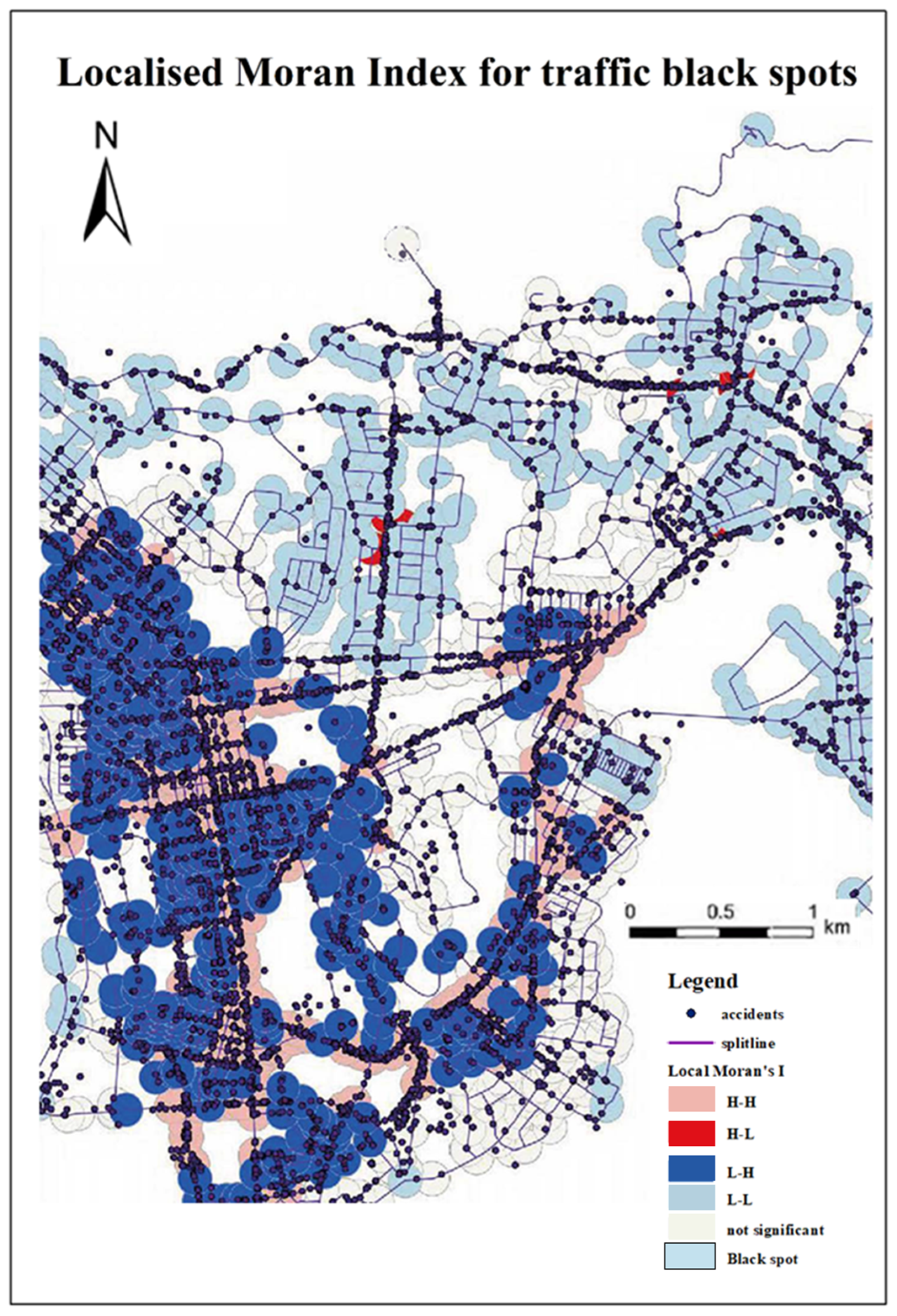
5.3.2. Local Moran’s I

The local Moran’s I is an index used to measure the local spatial autocorrelation of each geographic unit. The local Moran’s I is constructed for the traffic black spots at road intersections in the Kowloon Peninsula region of Hong Kong, and it identifies the spatial aggregation characteristics by comparing the attributes of each road intersection and its neighboring road intersections. Unlike the global Moran’s I, the local Moran’s I can help to identify the geographic units with local aggregation of the traffic black spots at the road intersections in the Kowloon Peninsula region of Hong Kong and reveal the spatial distribution of the traffic black spots at the road intersection patterns and heterogeneity.
The results in Table 26 indicate that there are four types of results, such as this is a traffic black spot aggregation area, a non-traffic black spot aggregation area, and so on, in the local distribution of traffic black spots at road intersections in the Kowloon Peninsula region of Hong Kong. Among them, the non-traffic black spot aggregation area is the most significant.
Table 26. Number of distributions of each cluster set of localized local Moran’s I for traffic black spots.
Figure 26 shows the spatial clustering distribution of traffic black spots at road intersections in the Kowloon Peninsula region of Hong Kong. The pink part represents the traffic black spot aggregation area, the light blue part represents the non-traffic black spot aggregation area, the red part represents the area where the traffic black spot aggregation area is surrounded by the non-traffic black spot aggregation area, and the dark blue part represents the area where the non-traffic black spot aggregation area is surrounded by the traffic black spot aggregation area. The non-traffic black spot agglomeration area is mainly concentrated on highways, where there are fewer people and buildings, and this physical environment leads to fewer traffic accidents and less possibility of becoming a traffic black spot, while the high traffic black spot agglomeration area is mainly concentrated in the Yau Tsim Mong District, where there is a dense road network, with a transportation junction, and a dense population and buildings, which have an agglomeration effect and lead to a greater probability of traffic accidents, leading it to become a traffic black spot. The probability of traffic accidents becomes greater, resulting in a higher probability of it becoming a traffic black spot. From the perspective of spatial correlation, it can be understood that the clustering area of a traffic black spot also affects the traffic safety of the surrounding area, resulting in a higher likelihood of traffic accidents.
Figure 26. Localized local Moran’s I for traffic black spots.

5.3.3. Summary of Spatial Correlation of Traffic Black Spots

The global Moran index analysis of traffic black spots at road intersections indicates that the distribution of traffic black spots is visibly spatially aggregated and positively correlated in the whole Kowloon Peninsula area. The local Moran index analysis of traffic black spots at road intersections indicates that there are visible traffic black spot aggregation areas and non-traffic black spot aggregation areas, which also indicates that adjacent road intersections will influence each other, increasing or decreasing the likelihood of each other becoming traffic black spots.
The above experiments show that there exists a spatial correlation of traffic black spots at road intersections in the Kowloon Peninsula region of Hong Kong, i.e., adjacent road intersections will affect each other in terms of their probability of becoming traffic black spots. Based on this situation, this paper improves the recognition method of road intersection traffic black spots, constructs a traffic black spot network topology, takes road intersections as nodes, uses the connecting lines between nodes as edges of the network, and the built environment of road intersections as node features, and uses the GCNN graphical convolutional neural network for traffic black spot recognition, which is a better way to perform contextual learning and feature aggregation of neighboring node information, and achieve better traffic black spot recognition.

5.4. GCNN-Based Model Experiment and Result Analysis

(1)
Experimental results
The data are divided randomly and the ratio of data in the training set and test set is 8:1:1. The accuracy of the test set is close to 90% and the Loss value is 0.43. This is shown in Figure 27.
Figure 27. Graph of the result of GCNN model to recognize traffic black spots.
The results of the graphical convolutional neural network for traffic black spot identification at road intersections are visualized in 2D space, as shown in Figure 28.
Figure 28. Visualization of the results of GCNN model to identify traffic black spots.
According to the experimental results of the graph convolutional neural network, it can be found that the GCNN model can be better used in the identification of traffic black spots. Through the extraction of semantic information between the built environment features of adjacent road intersections, the accuracy of the identification of traffic black spots has been improved to a certain extent, and the model value Loss has decreased significantly, which also confirms that, in daily life, the built environment is more similar between the neighboring roads and that, when a traffic accident occurs in a certain place, it brings about the negative effects of vehicular congestion, crowd gathering, and other negative effects which will be transmitted to the neighboring roads, which will make the probability of the occurrence of traffic accidents greatly increased.

6. Discussion

In this paper, based on the street view image data, we use the semantic segmentation model to obtain the built environment features of urban roads, take the road intersection as the research unit, carry out the research idea of traffic black spot identification and its cause analysis, construct a model for identifying traffic black spots based on the built environment of adjacent road intersections, and broaden the research idea of traffic black spot identification. The research results of this paper are summarized as follows: (1) In this paper, the Tencent Street View platform and Python crawler technology are used to obtain the street view image data of Hong Kong’s Kowloon area, and deep learning semantic segmentation technology is used to construct the built environment features of urban road intersections and define the concept of traffic black spots. (2) In this paper, based on the set of built environment features of road intersections, the support vector machine model, gradient boosting model, random forest model, and fully connected neural network model are applied to identify traffic black spots at road intersections, and the experimental results show the feasibility of identifying traffic black spots at road intersections based on the street view image data, and that their experimental accuracy can reach 87%. (3) In this paper, based on the above experiments, considering that the interconnection between the built environment features of adjacent road intersections will have an impact on the identification of traffic black spots, the traffic accident data and street view image data are processed, and the graph convolutional neural network model is used to identify traffic black spots at intersections and achieves better experimental performance. (4) This paper uses principal component analysis to analyze in detail several features that have the greatest impact on the formation of traffic black spots at urban road intersections, such as buildings, billboards, sky, greenery, etc., so that the traffic management department and the urban planning department can regulate the density of building development, pedestrian and vehicular flow, billboards, and greenery according to these findings.
We acknowledge three major limitations of this work and point out three directions for future work. (1) The scope of this paper is limited to the study of only one region, Kowloon Peninsula, Hong Kong, and only road intersections were selected as the study unit, resulting in a small amount of data. In the future, we will continue to expand the size of the whole dataset so that the results will be more reliable and convincing. (2) Secondly, this paper did not consider the time division in the process of identifying traffic black spots. Since most people have different travelling purposes on weekdays and weekends, and the situation of the morning and evening rush hours on weekdays is very different from other times of the day when people and traffic gather, all these factors may affect the distribution of traffic black spots; therefore, in the next stage of this study, the identification of traffic black spots by time period can be more refined to propose corresponding preventive measures to achieve “one point one policy”. (3) This paper is not comprehensive enough in the research and analysis of data. In the process of data collection, the current traffic management department is not able to collect all the information of the accident correctly, there is a part of the data which cannot be recorded by the precise geographic coordinates, and the attributes of the existing data on traffic accidents are not perfect, such as the lack of records on the characteristics of the vehicles and people involved, which will have an impact on the analysis of the causes of the traffic black spots.

7. Conclusions and Future Work

This study focuses on the recognition and causal analysis of black spots in road intersections using street view images. The research methodology revolves around utilizing street view image data as a foundation and employing a semantic segmentation model to extract the characteristics of the urban roads’ built environment. Specifically, this study adopts road intersections as the primary research unit to conduct the identification and cause analysis of traffic black spots. It innovatively constructs a model that identifies traffic black spots based on the built environment of adjacent road intersections, thereby expanding the current understanding of traffic black spot identification. The proposed model and accompanying research offer a novel perspective for traffic management authorities to effectively address traffic safety concerns. By leveraging insights from this study, it becomes possible to mitigate the occurrence of traffic accidents and reduce the probability of developing traffic black spots within the urban built environment.

Author Contributions

Conceptualization, L.T. and C.L.; methodology, L.T. and C.L.; software, C.L. and S.H.; validation, Y.W. and L.T.; formal analysis, Y.W.; investigation, C.L. and M.H.; resources, M.H. and S.H.; data curation, S.H. and M.H.; writing—original draft preparation, C.L.; writing—review and editing, L.T. and Y.W.; visualization, W.L. and S.H.; supervision, L.T.; project administration, Y.W.; and funding acquisition, L.T. All authors have read and agreed to the published version of the manuscript.

Funding

This research was funded by the Opening Fund of Hubei Key Laboratory of Intelligent Vision-Based Monitoring for Hydroelectric Engineering, grant number 2022SDSJ04; the Open Research Project of The Hubei Key Laboratory of Intelligent Geo-Information Processing, grant number KLIGIP-2022-A02.

Institutional Review Board Statement

Not applicable.

Data Availability Statement

The data presented in this study are available on request from the corresponding author. The data are not publicly available due to privacy.

Acknowledgments

Special thanks go to the editor and anonymous reviewers of this paper for their constructive comments.

Conflicts of Interest

The authors declare no conflicts of interest.

References

  1. van Hoof, J.; Marston, H.R.; Kazak, J.K.; Buffel, T. Ten questions concerning age-friendly cities and communities and the built environment. Build. Environ. 2021, 199, 107922. [Google Scholar] [CrossRef]
  2. Al-Obaidi, K.M.; Hossain, M.; Alduais, N.A.; Al-Duais, H.S.; Omrany, H.; Ghaffarianhoseini, A. A review of using IoT for energy efficient buildings and cities: A built environment perspective. Energies 2022, 15, 5991. [Google Scholar] [CrossRef]
  3. Feng, R.; Feng, Q.; Jing, Z.; Zhang, M.; Yao, B. Association of the built environment with motor vehicle emissions in small cities. Transp. Res. Part D Transp. Environ. 2022, 107, 103313. [Google Scholar] [CrossRef]
  4. Ge, H.; Dong, L.; Huang, M.; Zang, W.; Zhou, L. Adaptive kernel density estimation for traffic accidents based on improved bandwidth research on black spot identification model. Electronics 2022, 11, 3604. [Google Scholar] [CrossRef]
  5. Liu, D.; Jiang, Y.; Wang, R.; Lu, Y. Establishing a citywide street tree inventory with street view images and computer vision techniques. Comput. Environ. Urban Syst. 2023, 100, 101924. [Google Scholar] [CrossRef]
  6. Huang, J.; Obracht-Prondzynska, H.; Kamrowska-Zaluska, D.; Sun, Y.; Li, L. The image of the City on social media: A comparative study using “Big Data” and “Small Data” methods in the Tri-City Region in Poland. Landsc. Urban Plan. 2021, 206, 103977. [Google Scholar] [CrossRef]
  7. Singh, N.; Katiyar, S.K. Application of geographical information system (GIS) in reducing accident blackspots and in planning of a safer urban road network: A review. Ecol. Inform. 2021, 66, 101436. [Google Scholar] [CrossRef]
  8. Wang, Z.Z.; Lu, Y.N.; Zou, Z.H.; Ma, Y.H.; Wang, T. Applying OHSA to Detect Road Accident Blackspots. Int. J. Environ. Res. Public Health 2022, 19, 16970. [Google Scholar] [CrossRef] [PubMed]
  9. Feng, G.; Zou, G.; Piga, B.E.A.; Hu, H. The Validity of Street View Service Applied to Ambiance Perception of Street: A Comparison of Assessment in Real Site and Baidu Street View. In Advances in Industrial Design, Proceedings of the AHFE 2021 Virtual Conferences on Design for Inclusion, Affective and Pleasurable Design, Interdisciplinary Practice in Industrial Design, Kansei Engineering, and Human Factors for Apparel and Textile Engineering, Virtual Event, New York, NY, USA, 25–29 July 2021; Springer International Publishing: Cham, Switzerland, 2021; pp. 740–748. [Google Scholar]
  10. Han, Y.; Zhong, T.; Yeh, A.G.; Zhong, X.; Chen, M.; Lü, G. Mapping seasonal changes of street greenery using multi-temporal street-view images. Sustain. Cities Soc. 2023, 92, 104498. [Google Scholar] [CrossRef]
  11. Zhang, G.; Yi, J.; Yuan, J.; Li, Y.; Jin, D. DAS: Efficient Street View Image Sampling for Urban Prediction. ACM Trans. Intell. Syst. Technol. 2023, 14, 1–20. [Google Scholar] [CrossRef]
  12. Liu, L.; Zhou, B.; Zhao, J.; Ryan, B.D. C-IMAGE: City cognitive mapping through geo-tagged photos. GeoJournal 2016, 81, 817–861. [Google Scholar] [CrossRef]
  13. Zhang, F.; Zhang, D.; Liu, Y.; Lin, H. Representing place locales using scene elements. Comput. Environ. Urban Syst. 2018, 71, 153–164. [Google Scholar] [CrossRef]
  14. Jahan, A.; Abbaspour, A.; Safakhah, S. A hybrid method based on P and P′ control chart for identifying hotspots. Qual. Reliab. Eng. Int. 2021, 37, 3493–3511. [Google Scholar] [CrossRef]
  15. Ambo, T.B.; Ma, J.; Fu, C.; Atumo, E.A. Investigating road conditions of crash blackspots in Addis Ababa, Ethiopia: A random parameters negative binomial model. Int. J. Crashworthiness 2023, 1–12. [Google Scholar] [CrossRef]
  16. Fiorentini, N.; Losa, M. Long-term-based road blackspot screening procedures by machine learning algorithms. Sustainability 2020, 12, 5972. [Google Scholar] [CrossRef]
  17. Clifton, K.J.; Smith, A.D.L.; Rodriguez, D. The development and testing of an audit for the pedestrian environment. Landsc. Urban Plan. 2007, 80, 95–110. [Google Scholar] [CrossRef]
  18. Day, K.; Boarnet, M.; Alfonzo, M.; Forsyth, A. The Irvine–Minnesota inventory to measure built environments: Development. Am. J. Prev. Med. 2006, 30, 144–152. [Google Scholar] [CrossRef]
  19. Pikora, T.J.; Bull, F.C.; Jamrozik, K.; Knuiman, M.; Giles-Corti, B.; Donovan, R.J. Developing a reliable audit instrument to measure the physical environment for physical activity. Am. J. Prev. Med. 2002, 23, 187–194. [Google Scholar] [CrossRef]
  20. Rundle, A.G.; Bader, M.D.; Richards, C.A.; Neckerman, K.M.; Teitler, J.O. Using Google Street View to audit neighborhood environments. Am. J. Prev. Med. 2011, 40, 94–100. [Google Scholar] [CrossRef]
  21. Bromm, K.N.; Lang, I.M.; Twardzik, E.E.; Antonakos, C.L.; Dubowitz, T.; Colabianchi, N. Virtual audits of the urban streetscape: Comparing the inter-rater reliability of GigaPan® to Google Street View. Int. J. Health Geogr. 2020, 19, 31. [Google Scholar] [CrossRef]
  22. Badland, H.M.; Opit, S.; Witten, K.; Kearns, R.A.; Mavoa, S. Can virtual streetscape audits reliably replace physical streetscape audits? J. Urban Health 2010, 87, 1007–1016. [Google Scholar] [CrossRef] [PubMed]
  23. Wilson, J.S.; Kelly, C.M.; Schootman, M.; Baker, E.A.; Banerjee, A.; Clennin, M.; Miller, D.K. Assessing the built environment using omnidirectional imagery. Am. J. Prev. Med. 2012, 42, 193–199. [Google Scholar] [CrossRef]
  24. Clarke, P.; Ailshire, J.; Melendez, R.; Bader, M.; Morenoff, J. Using Google Earth to conduct a neighborhood audit: Reliability of a virtual audit instrument. Health Place 2010, 16, 1224–1229. [Google Scholar] [CrossRef]
  25. Hadayeghi, A.; Shalaby, A.S.; Persaud, B.N. Development of planning level transportation safety tools using Geographically Weighted Poisson Regression. Accid. Anal. Prev. 2010, 42, 676–688. [Google Scholar] [CrossRef] [PubMed]
  26. Isola, P.D.; Bogert, J.N.; Chapple, K.M.; Israr, S.; Gillespie, T.L.; Weinberg, J.A. Google Street View assessment of environmental safety features at the scene of pedestrian automobile injury. J. Trauma Acute Care Surg. 2019, 87, 82–86. [Google Scholar] [CrossRef]
  27. Hanson, C.S.; Noland, R.B.; Brown, C. The severity of pedestrian crashes: An analysis using Google Street View imagery. J. Transp. Geogr. 2013, 33, 42–53. [Google Scholar] [CrossRef]
  28. Johnson, N.S.; Gabler, H.C. Injury outcome in crashes with guardrail end terminals. Traffic Inj. Prev. 2015, 16, 103–108. [Google Scholar] [CrossRef]
  29. Wang, D.; Krebs, E.; Vissoci, J.R.N.; de Andrade, L.; Rulisa, S.; Staton, C.A. Built environment analysis for road traffic crash hotspots in Kigali, Rwanda. Front. Sustain. Cities 2020, 2, 17. [Google Scholar] [CrossRef]
  30. Qin, K.; Xu, Y.; Kang, C.; Kwan, M. A graph convolutional network model for evaluating potential congestion spots based on local urban built environments. Trans. GIS 2020, 24, 1382–1401. [Google Scholar] [CrossRef]
  31. Long, J.; Shelhamer, E.; Darrell, T. Fully convolutional networks for semantic segmentation. In Proceedings of the IEEE Conference on Computer Vision and Pattern Recognition, Boston, MA, USA, 7–12 June 2015; pp. 3431–3440. [Google Scholar]
  32. Badrinarayanan, V.; Kendall, A.; Cipolla, R. Segnet: A deep convolutional encoder-decoder architecture for image segmentation. IEEE Trans. Pattern Anal. Mach. Intell. 2017, 39, 2481–2495. [Google Scholar] [CrossRef]
  33. Ronneberger, O.; Fischer, P.; Brox, T. U-net: Convolutional networks for biomedical image segmentation. In Medical Image Computing and Computer-Assisted Intervention–MICCAI 2015: 18th International Conference, Proceedings, Part III 18, Munich, Germany, 5–9 October 2015; Springer International Publishing: Cham, Switzerland, 2015; pp. 234–241. [Google Scholar]
  34. Chen, L.-C.; Papandreou, G.; Kokkinos, I.; Murphy, K.; Yuille, A.L. Deeplab: Semantic image segmentation with deep convolutional nets, atrous convolution, and fully connected crfs. IEEE Trans. Pattern Anal. Mach. Intell. 2017, 40, 834–848. [Google Scholar] [CrossRef] [PubMed]
  35. Zhao, H.; Shi, J.; Qi, X.; Wang, X.; Jia, J. Pyramid scene parsing network. In Proceedings of the IEEE Conference On Computer Vision and Pattern Recognition, Honolulu, HI, USA, 21–26 July 2017; pp. 2881–2890. [Google Scholar]
  36. Fu, J.; Liu, J.; Tian, H.; Li, Y.; Bao, Y.; Fang, Z.; Lu, H. Dual attention network for scene segmentation. In Proceedings of the IEEE/CVF Conference on Computer Vision and Pattern Recognition, Long Beach, CA, USA, 15–20 June 2019; pp. 3146–3154. [Google Scholar]
  37. Elvik, R. State-of-the-Art Approaches to Road Accident Black Spot Management and Safety Analysis of Road Networks; Transportøkonomisk Institutt: Oslo, Norway, 2007. [Google Scholar]
  38. Lord, D.; Persaud, B.N. Estimating the safety performance of urban road transportation networks. Accid. Anal. Prev. 2004, 36, 609–620. [Google Scholar] [CrossRef]
  39. Geurts, K.; Wets, G. Black spot analysis methods: Literature review. Economics 2003, 1, 32. [Google Scholar]
  40. Wright, C.C.; Abbess, C.R.; Jarrett, D.F. Estimating the regression-to-mean effect associated with road accident black spot treatment: Towards a more realistic approach. Accid. Anal. Prev. 1988, 20, 199–214. [Google Scholar] [CrossRef] [PubMed]
  41. Iqbal, A.; Rehman, Z.U.; Ali, S.; Ullah, K.; Ghani, U. Road traffic accident analysis and identification of black spot locations on highway. Civ. Eng. J. 2020, 6, 2448–2456. [Google Scholar] [CrossRef]
  42. Jorgensen, N.O. Statistical detection of accident blackspots. In Proceedings of the OTA-PIARC 11th Study Week in Transportation and Safety, Brussels, Belgium, 1972. [Google Scholar]
  43. Yulong, P. The outstanding factor method to differentiate the black spot of the road. In Proceedings of the 15th International Road Federation World Meeting, Bangkok, Thailand, 14–19 June 2005. [Google Scholar]
  44. Geurts, K.; Wets, G.; Brijs, T.; Vanhoof, K. Identification and ranking of black spots: Sensitivity analysis. Transp. Res. Rec. 2004, 1897, 34–42. [Google Scholar] [CrossRef]
  45. Nguyen, H.H.; Taneerananon, P.; Luathep, P. Approach to identifying black spots based on potential saving in accident costs. Eng. J. 2016, 20, 109–122. [Google Scholar] [CrossRef]
  46. Nguyen, H.H.; Taneerananon, P.; Koren, C.; Iamtrakul, P. Safety-potential-based black spot safety management approach: A case study in Ho Chi Minh City. J. East. Asia Soc. Transp. Stud. 2013, 10, 1991–2009. [Google Scholar]
  47. Yao, Y.; Liang, Z.; Yuan, Z.; Liu, P.; Bie, Y.; Zhang, J.; Wang, R.; Wang, J.; Guan, Q. A human-machine adversarial scoring framework for urban perception assessment using street-view images. Int. J. Geogr. Inf. Sci. 2019, 33, 2363–2384. [Google Scholar] [CrossRef]
Disclaimer/Publisher’s Note: The statements, opinions and data contained in all publications are solely those of the individual author(s) and contributor(s) and not of MDPI and/or the editor(s). MDPI and/or the editor(s) disclaim responsibility for any injury to people or property resulting from any ideas, methods, instructions or products referred to in the content.

Article Metrics

Citations

Article Access Statistics

Multiple requests from the same IP address are counted as one view.